Bargaining in Stationary Networks
The MIT Faculty has made this article openly available.
Please share
how this access benefits you. Your story matters.
Citation
Manea, Mihai. “Bargaining in Stationary Networks.” American
Economic Review 101.5 (2011): 2042–2080. Web. © 2011 American
Economic Association.
As Published
http://dx.doi.org/10.1257/aer.101.5.2042
Publisher
American Economic Association
Version
Final published version
Citable link
http://hdl.handle.net/1721.1/73022
Terms of Use
Article is made available in accordance with the publisher's
policy and may be subject to US copyright law. Please refer to the
publisher's site for terms of use.
=10.1257/aer.101.5.2042
2042
Competitive equilibrium theory assumes large and anonymous markets in which every buyer can trade with every seller. Underlying these assumptions are standard goods and services that may be traded at low transaction costs by agents who are not in specific relationships with one another. However, in many markets goods
and services are heterogeneous (e.g., cars, apartments) or need to be tailored to
particular needs (e.g., manufacturing inputs, technical support). Furthermore,
trad-ing opportunities may depend on transportation costs, social relationships, infor-mation, advertising, trust, technological compatibility, joint business opportunities, free trade agreements, etc. In such cases it is natural to model the market using a
network, where only pairs of connected agents may engage in exchange.
New theories are needed to explore the influence of the network structure on
market outcomes. Many questions arise: How does an agent’s position in the net-work determine his bargaining power and the local prices he faces? Who trades with whom and on what terms? When are prices uniform in the network?
One possible conjecture is that an agent’s bargaining power is determined by his (relative) number of connections in the network. However, this simple theory is
implausible. Consider the network of four sellers (located at the top nodes) and nine
buyers (located at the bottom nodes) depicted in Figure 1. Assume that each seller
supplies one unit of a homogeneous indivisible good, each buyer demands one unit of the good, and all buyers have identical values for the good. The buyer located in the middle has the largest number of links in the network, as he is connected to each
* Department of Economics, MIT, 50 Memorial Drive, Cambridge, MA 02142 (e-mail: [email protected]). I am grateful to Drew Fudenberg for continual guidance in approaching this project and to Dilip Abreu for valuable per-spectives. I thank Jeff Ely, Sambuddha Ghosh, Faruk Gul, John Hatfield, Fuhito Kojima, Michael Ostrovsky, Marcin Peski, Al Roth, Satoru Takahashi, Rakesh Vohra, Asher Wolinsky, and Muhamet Yildiz for helpful comments.
† To view additional materials, visit the article page at http://www.aeaweb.org/articles.php?doi=10.1257/aer.101.5.2042.
Bargaining in Stationary Networks
†By Mihai Manea*
We study an infinite horizon game in which pairs of players
con-nected in a network are randomly matched to bargain. Players who
reach agreement are replaced by new players at the same positions
in the network. We show that all equilibria are payoff equivalent. The
payoffs and the set of agreement links converge as players become
patient. Several new concepts—mutually estranged sets, partners,
and shortage ratios—provide insights into the relative strengths
of the positions in the network. We develop a procedure to
deter-mine the limit equilibrium payoffs for all players. Characterizations
of equitable and nondiscriminatory networks are also obtained.
of the four sellers. Yet every seller has monopoly power over two other buyers whom he can extort, even if trade with the better connected buyer is unattainable. Hence the middle buyer is not able to extract a large fraction of the surplus from any seller despite his relatively large number of connections.
The example above illustrates that the relative strengths of the positions in a net-work are highly interdependent. An agent’s bargaining power does not depend only on the number of his partners, but also on the identities and bargaining power of his partners. Each partner’s bargaining power depends in turn on the strengths of his cor-responding partners, and so forth. An adequate measure of bargaining power needs to reflect the global network structure.
A recent book by Matthew O. Jackson (2008) surveys the emerging field of social
and economic networks and concludes that several central issues remain unsolved.
There are important open questions regarding how network structure
affects the distribution of the benefits that accrue to different actors in a
network (p. 459).
In particular, Jackson notes that analyzing “a noncooperative game that completely
models the bargaining process through which ultimate payoffs are determined […]
is usually intractable” (p. 412). The present paper attempts to fill this gap using a
noncooperative model of decentralized bilateral bargaining in networks. Our model is tractable and provides answers to the questions raised earlier.
The benchmark model is as follows. We consider a network where each pair of players connected by a link can jointly produce a unit surplus. The network gener-ates the following infinite horizon discrete time bargaining game. Each period a link is selected according to some probability distribution, and one of the two matched players is randomly chosen to make an offer to the other player specifying a division of the unit surplus between themselves. If the offer is accepted, the two players exit the game with the shares agreed on. We make the following steady state assumption. The two players who reached agreement are replaced in the next period by two new players at the same positions in the network. If the offer is rejected, the two players remain in the game for the next period. All players have a common discount factor.
The steady state assumption captures the idea that in many markets agents face stationary distributions of bargaining opportunities. In such cases, some agents take similar positions in relationships and transactions at different points in time. Our benchmark model provides a stylized depiction of steady states in an economy with multiple populations and a complex pattern of trading opportunities. In the multiple
Figure 1. The Position with the Largest Number of Connections Is Not Necessarily the Strongest
population interpretation, each node corresponds to a population of identical agents, and the network represents the structure of interactions among populations. From this perspective, our setting constitutes an extension of Ariel Rubinstein and Asher
Wolinsky’s (1985) fundamental model of bargaining in stationary markets with two
populations.
Indeed, the results carry over to a model in the spirit of Douglas M. Gale’s (1987),
where every period a continuum of players is present at each node in the network, and a positive measure of player pairs are matched to bargain across each link. While in the benchmark model the replacement assumption entails that every period an inflow of agents matches the stochastic endogenous outflow of agents reaching agreements in equilibrium, in the multiple population version the steady state analy-sis involves a deterministic inflow. This enables us to investigate how the size of the population at each node is determined in a steady state of an economy with
exog-enously specified inflows of agents into the network. Manea (2010) studies a more general model of multipopulation bargaining with an emphasis on nonstationary markets.
Depending on the application, populations may correspond to buyers and sellers
of used cars with specific parameters (brand, mileage, manufacturing year, fuel
effi-ciency, warranty, etc.); renters with specific demands (in terms of location, number
of bedrooms, recent renovation, dishwasher availability, etc.) and the corresponding
landlords; firms with different types of production technologies and workers with particular training and job preferences; importers and exporters who trade goods that meet certain quality standards. In the former two applications, populations can be further divided according to exposure to various advertising platforms, demo-graphics, and locations of buyers and sellers. In the latter, trading companies are differentiated by the ability to meet the requirements of particular markets, trade permits, and business connections.
In general, a population is defined by a category of agents who share the same relevant attributes for the market under consideration. The network of exchange is determined by the compatibility of the factors describing various populations. Background elements such as word-of-mouth communication, consumer protection laws, transportation costs, and trade agreements also shape the network. For example, a prospective renter is effectively connected only to landlords who meet his apart-ment search criteria and whom he finds through acquaintances, real estate agencies, or advertisements. In markets with multiple populations, the steady state assumption translates into the stationarity of the distribution of buyer and seller types.
Suppose that in the underlying network a certain group of buyers can trade only with a relatively small number of sellers. One might surmise that these sellers can use their oligopoly power to capture a significant fraction of the gains from trade. This is not necessarily the case for each seller involved. Due to network asymmetries, the sellers may have unequal bargaining power. Indeed, some subsets of the original oligopoly may face higher demand and exert more market power relative to others. For instance, if a subset of the sellers is connected to only one of the buyers, then the buyer can exploit his monopsony power. Some of the remaining sellers will form an oligopoly with greater market power than initially assumed. Other delicate issues arise. For example, overlapping oligopolies may cater to a common customer base or split up into several smaller oligopolies with varying degrees of bargaining power.
The set of oligopolies and the price distribution emerging in equilibrium depend on the network structure in a complex fashion. The partition of the market into oligopolies and the relative strengths of the oligopolies are determined endoge-nously via decentralized bargaining. Our analysis reveals that the most powerful oligopolies—the ones with the lowest seller-to-buyer ratio—drive market outcomes. Roughly speaking, for patient agents, the network is decomposed into a series of oligopolies, which are ordered decreasingly according to market power. Each oli-gopoly in the list includes all buyers and sellers with extremal payoffs among those not involved in the preceding oligopolies.
I. Outline of the Results
We assume that the network structure is common knowledge and all players have perfect information about the events preceding any of their decision nodes in the
game. The equilibrium concept we use is subgame perfect equilibrium.1
In Section III, we show that for every discount factor the equilibrium payoff of every player present in the game at the beginning of any period is uniquely
deter-mined by his position in the network (Theorem 1). For all but a finite number of
discount factors, there exists a partition of the set of links into equilibrium
agree-ment and disagreeagree-ment links (Proposition 1). In every equilibrium, after any history,
a pair of players connected by an equilibrium agreement link reaches an agreement when matched to bargain, and the terms of the agreement are uniquely pinned down by the positions in the network of the proposer and the responder. Players con-nected by disagreement links never reach agreement. We prove that there exists a limit equilibrium agreement network that describes the set of agreement links for sufficiently high discount factors. Also, the equilibrium payoffs converge as players
become patient (Theorem 2).
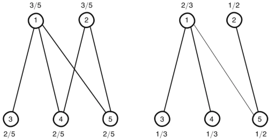
For an illustration, consider the bargaining game on the five-player network g 1
shown in Figure 2, where all links are selected for bargaining with equal probability.2
For every discount factor there is a unique equilibrium, with agreement network
g1 . In equilibrium every match ends in agreement because players 4 and 5 cannot
be monopolized by either player 1 or 2. The limit equilibrium payoffs are 3/5 for
players 1 and 2, and 2/5 for players 3, 4, and 5. The limit equilibrium agreement
network coincides with g 1 .
Consider next the game induced by the network g 2 , which is obtained from g 1
by removing the link (2, 4). We assume again that every link is drawn for bargaining
with the same probability. For low discount factors there exists a unique
equilib-rium, with the agreement network given by g 2 . However, for high discount factors,
players 1 and 5 do not reach an agreement in equilibrium when matched to bargain. The intuition is that player 1 can extort players 3 and 4, since these two players do not have other bargaining partners. Player 1 cannot extract as much surplus from player 5, since 5 has monopoly over player 2. The limit equilibrium payoffs are
1 Section III discusses the robustness of the results to some features of the information structure and equilib-rium requirements.
2 In all figures, limit equilibrium payoffs for each player are represented next to the corresponding node, and limit equilibrium agreement and disagreement links are drawn as thick and thin line segments, respectively.
2/3 for player 1, 1/3 for players 3 and 4, and 1/2 for players 2 and 5. The limit
equilibrium agreement network consists of all links of g 2 except (1, 5). The
equilib-ria of the bargaining games on the networks g 1 and g 2 for all discount factors are
described in detail in Example 1 from Section III.
The main objective is to characterize the limit equilibrium payoffs for every net-work. The following essential observation is presented in Section IV. Consider a set of players who are pairwise disconnected in the limit equilibrium agreement network and the set of players with whom these players share limit agreement links. We refer to players in the former set as mutually estranged and to ones in the latter as
partners. As players become patient, the partners have control over the (equilibrium)
relevant bargaining opportunities of the mutually estranged players. For high dis-count factors, since the estranged players can reach agreements only in equilibrium with the partners, the mutually estranged set is weak if the partners are relatively scarce. The appropriate measure of the strength of a mutually estranged set proves to be the simplest that springs to mind—the shortage ratio, which is defined as the ratio of the number of partners to estranged players.
For example, in the network g 1 the shortage ratios of the mutually estranged sets
{3, 4} and {3, 4, 5} are 1 and 2/3, respectively, since the partner set is {1, 2} in either
case. In the network g 2 the shortage ratios of the mutually estranged sets {3, 4} and
{3, 4, 5} are 1/2 and 2/3, respectively, since the corresponding partner sets are {1}
and {1, 2}, respectively. The determination of the partners for the mutually estranged
sets considered here is based on the aforementioned limit equilibrium agreement
subnetworks for the bargaining games on the networks g 1 and g 2 .
The concepts of mutually estranged sets, partners, and shortage ratios play a key role in the prediction of bargaining power. Formally, the shortage ratio measures the strength of a mutually estranged set in the following sense. For every set of mutually estranged players and their partners, the ratio of the limit equilibrium payoffs of the worst-off estranged player and the best-off partner is not larger than the shortage
ratio of the mutually estranged set (Theorem 3). The result yields an upper (lower)
bound for the limit payoff of the worst-off estranged player (best-off partner).
There may be a multitude of mutually estranged sets, and it is not immediately clear which, if any, of the corresponding bounds for the limit equilibrium payoffs
Figure 2. Networks G1(left) and G2
1 2 1 2 5 5 4 4 3 3 3/5 3/5 2/5 2/5 2/5 1/3 1/3 1/2 1/2 2/3
are binding. One delicate step toward the main result (Theorem 4) is the idea that the bounds generated by a set of mutually estranged players and their partners need to be binding unless the worst-off estranged player is part of an even weaker mutually estranged set, and the best-off partner is part of an even stronger partner set. Based
on this intuition, we prove that the extreme bounds—the ones derived from the
(larg-est) mutually estranged set that minimizes the shortage ratio and the corresponding
partners—must bind.3 The two sets of players associated with these bounds have
extremal limit equilibrium payoffs and induce an oligopoly subnetwork enclosing all their limit agreement links. Thus, for high discount factors, the partners act as an oligopoly that corners and extorts the estranged players. In the equilibrium limit, surplus within the oligopoly subnetwork is divided according to the shortage ratio of the mutually estranged players with respect to their partners, with all players on each side receiving identical payoffs.
Section V develops an algorithm that sequentially determines the limit equilib-rium payoffs of all players based on the ideas above. At each step, the algorithm determines the union of all mutually estranged sets with the lowest shortage ratio and removes the corresponding estranged players and their partners. Within the identified extremal oligopoly subnetwork surplus is divided between the two sides according to the shortage ratio. The algorithm stops when all players have been removed or when the lowest shortage ratio is greater than or equal to 1. The latter
scenario corresponds to limit payoffs of 1/2 for the remaining players.
The limit equilibrium payoffs for the network g 2 are obtained by computing the
lowest shortage ratio to be 1/2, attained for the mutually estranged set {3, 4} with
the partner set {1}. Then the limit payoffs are 2/3 for player 1 and 1/3 for players 3
and 4. Once we remove players 1, 3, and 4, the lowest shortage ratio in the
remain-ing network is 1; hence, players 2 and 5 obtain limit payoffs of 1/2.
We can use the algorithm to investigate the uniformity of payoffs in a network. A network is called equitable if it does not create differentiated bargaining power as
players become patient; that is, all players have limit equilibrium payoffs of 1/2. In
Section VI we show that a network is equitable if and only if it is quasi-regularizable; another equivalent condition is that the network have an edge cover which is the
dis-joint union of a matching and odd cycles (Theorem 5).
Section VII restricts attention to buyer-seller networks and provides a more
straightforward characterization of the equilibrium limit (Theorem 4 BS). Shortage
ratios smaller than 1 and limit payoffs of 1/2 do not play a special role in the results
for buyer-seller networks. We also analyze nondiscriminatory buyer-seller net-works, where the limit payoffs of all buyers are identical. If the buyer-seller ratio is an integer, then the network is nondiscriminatory if and only if it can be covered by a disjoint union of clusters formed by one seller connected to a number of buyers
equal to the buyer-seller ratio (Theorem 6).
In Section VIII, we clarify the replacement assumption in the context of a mar-ket where there is a continuum of agents every period. Each node corresponds to a population of identical agents, and the network represents the pattern of exchange 3 Our analysis reveals that the lowest shortage ratio, when smaller than 1, may be computed by considering sets of pairwise disconnected players, along with their neighbors, in the original network rather than in the (a priori unknown) limit equilibrium agreement network.
opportunities between populations. In the analog stationary game for the multiple population setting, a constant measure of players is present at each node of the network in every period. The matching technology is such that, for each link in the network, a mass of pairs of players at the two endpoints is selected for bargain-ing. The steady state assumption delivering the stationary structure of the game is that the set of players from a given node who reach agreements is immediately replaced by an equal measure of new players at that node. Under this assumption, the steady state analysis of the benchmark model extends without difficulty.
The characterization of the equilibrium payoffs and agreements in the stationary game can be used to address the issue of determining a steady state when the set of potential market entrants is exogenously specified. Theorem 7 is a corollary of an
existence result established in the framework of Manea (2010). Suppose that there is
a constant stream of potential entrants at each node in the network. For any match-ing technology that varies continuously with the stationary distribution of agents in the market, there exist small entry costs for each node such that the resulting
economy has a steady state. Manea (2010) shows that strengthening this result to
apply for every set of small entry costs is not possible.
Rubinstein and Wolinsky (1985) and Gale (1987) analyze markets in steady state
abstracting away from existence issues and invoking replacement assumptions anal-ogous to ours. Similarly, the focus here is on the equilibrium outcomes of bargaining in stationary markets, rather than the mechanics of steady states. While it is useful to close the model with exogenous inflows as in the setting of Section VIII, the key contribution of this paper is the characterization of bargaining power in stationary networks developed in Sections II through VII.
Section IX reviews the related literature, and Section X concludes. An online Appendix discusses network stability with respect to the limit equilibrium payoffs, extensions of the results to heterogenous discount factors, and an example in which the bargaining protocol is asymmetric.
II. Framework
Let n denote the set of n players, n = {1, 2, … , n}. A network is an undirected
graph H = (V, E) with set of vertices V ⊂ n and set of edges—also called links—
E⊂ {(i, j) | i ≠ j ∈ V} such that ( j, i) ∈ E whenever (i, j) ∈ E.4 We identify the pairs
(i, j) and ( j, i), and use the shorthand ij or ji instead. We say that player i is
con-nected in H to player j, or i has an H link to j, if ij ∈ E. We regularly abuse notation
and write ij ∈ H for ij ∈ E. A network H′ = (V′, E′) is a subnetwork of H if V′ ⊂ V
and E′ ⊂ E. A network H′ = (V′, E′) is the subnetwork of H induced by V′ if E′ =
E⋂ (V′ × V′).
Fix a network g with vertex set n. Let ( p ij> 0 ) ij∈g be a matching technology
for g, which is a probability distribution over g’s links. A link ij in g is interpreted
as the ability of players i and j to jointly generate a unit surplus.5 Consider the
fol-lowing infinite horizon bargaining game generated by the network g. Each period
t= 0, 1, … a link ij in g is selected with probability p ij , and one of the players (the
4 Throughout the paper, ⊂ denotes weak inclusion; other authors prefer the symbol ⊆. 5 Without loss of generality, we assume that each player has at least one link in g.
proposer) i and j is chosen randomly (with equal probability) to make an offer to
the other player (the responder) specifying a division of the unit surplus between
themselves. If the responder accepts the offer, the two players exit the game with the
shares agreed upon. In period t + 1 two new players assume the same positions in
the network as i and j, respectively. If the responder rejects the offer, the two
play-ers remain in the game for the next period. In period t + 1 the game is played in the
same manner with the set of n players, consisting of the ones from period t, with the departing players replaced by new players if an agreement obtains in period t. All
players share a discount factor δ ∈ (0, 1). The game is denoted Γ δ .
Formally, there exists a sequence i 0 , i 1 , … , i τ , … of players of type i ∈ n (a
play-er’s type is defined by his position in the network). When player i τ exits the game
(following an agreement with another player), player i τ+1 replaces him the next
period.6 All players have common knowledge of the game, including the network
structure and the matching technology. We assume that players have perfect infor-mation of all the events preceding any of their decision nodes in the game. Possible relaxations of the informational assumptions regarding past bargaining outcomes are discussed in the next section.
There are three types of histories. We denote by h t a history of the game up to
(not including) time t, which is a sequence of t pairs of proposers and responders connected in g, with corresponding proposals and responses. We call such histories, and the subgames that follow them, complete. For simplicity, we assume that for every history players are labeled only by their type without reference to the index of
their copy. The index τ of the player of type i playing the game at time t following
the history h t can be recovered by counting the number of bargaining agreements
involving i along h t. Therefore, for each i ∈ n, a history h t uniquely determines the
player i τ present in the game at time t, and when there is no risk of confusion we
suppress the index τ. We denote by ( i τ) the set of complete histories, or subgames,
where i τ is the player of type i present in the game. We denote by ( h t ; i → j) the
history consisting of h t followed by nature selecting i to propose to j. We denote by
( h t ; i → j; x) the history consisting of ( h t ; i → j) followed by i offering x ∈ [ 0, 1] to j. A strategy σ i τ for player i τ specifies, for all j connected to i in g and all h t ∈ ( i τ ), the offer σ i τ ( h t ; i → j) that i makes to j following the history ( h t ; i → j), and the response σ i τ ( h t ; j → i; x) that i gives to j after the history ( h t ; j → i; x ). We allow for mixed strategies, hence σ i τ ( h t ; i → j) and σ i τ ( h t ; j → i; x) are probability
distributions over [ 0, 1] and {Yes, No}, respectively. In the context of our game, we
say that two strategy profiles are payoff equivalent if they induce identical payoffs for any player i τ , where i τ ’s payoff is evaluated as the expected value of his gains
from all the agreements discounted relative to his date of entry into the game (which
is not period 0 for τ ≥ 1). A strategy profile ( σ i τ ) i∈n, τ ≥ 0 is a subgame perfect
equilibrium of Γ δ if it induces Nash equilibria in subgames following every history
( h t ; i → j) and ( h t ; i → j; x).
6 The results extend to an alternative specification of the model where every period there is a continuum of play-ers at every node and a positive mass of playplay-ers is matched to bargain across each link. Section VIII develops this approach.
III. Essential Equilibrium Uniqueness and Discounting Asymptotics
We first show that across all equilibria of the bargaining game, the expected pay-off of every player present in any complete subgame is uniquely determined by his position in the network. The unique and stationary equilibrium payoffs associated with each player type may be used to describe the possible equilibrium outcomes of every bargaining encounter.
THEOREM 1: For every δ ∈ (0, 1), there exists a payoff vector ( v i* δ ) i∈n such that
for every subgame perfect equilibrium of Γ δ the expected payoff of player i τ in any ( i τ ) subgame is uniquely given by v i* δ for all i ∈ n, τ ≥ 0. For every equilibrium of Γ δ , in any subgame where i
τ is selected to make an offer to j τ ′ , the following
state-ments hold with probability one:
(i) if δ( v i* δ + v j* δ ) < 1 then i τ offers δ v j* δ and j τ ′ accepts; (ii) if δ( v i* δ + v j* δ ) > 1 then i τ makes an offer that j τ ′ rejects.
We can extend the conclusions of Theorem 1 to settings in which players do not have perfect information about all past matchings but still have common knowledge of the network structure. It may be that players know only their own history of inter-actions or know the history of all pairs matched to bargain but see the outcomes of only their own interactions. Players who reach agreements and exit the game may pass down information to the players who take their positions in the network. A player may learn that his bargaining partner has type i but be uncertain whether he is dealing with player i 0 , i 1 , …. In such settings, players need to form beliefs about the unrevealed bargaining outcomes. Extending the proof to show uniqueness of the sequential equilibrium payoffs for each player type under various information structures is straightforward. The uniqueness argument relies solely on the assump-tion that in every match the proposer knows the posiassump-tion of the responder in the
(commonly known) network.7
Manea (2010) establishes equilibrium payoff equivalence in markets with
mul-tiple populations where the probability that any two player types are matched at a given date is exogenous. Theorem 1 is a special case of that uniqueness result, and we omit its proof here. However, we present a partial argument showing that all
stationary equilibria in the current model are payoff equivalent. The ideas of the argument also play an important role in subsequent results.
A strategy profile ( σ i τ ) i∈n, τ ≥ 0 is stationary if each player’s strategy at any time t depends exclusively on his position in the network and the play of the game in period
t, that is, σ i τ ( h t ; i → j) = σ i τ ′ ( h ′ ; i → j) and σ t′ i τ ( h t ; j → i; x) = σ i τ ′ ( h′ t ′ ; j → i; x) for all ij ∈ g, x ∈ [ 0, 1 ], τ, τ ′ ≥ 0, h t∈ ( i τ ), h t ′ ∈ ( i ′ τ ′ ). A stationary
equilib-rium is a subgame perfect equilibequilib-rium in stationary strategies.
Let σ be a stationary equilibrium of Γ δ . Under σ, for every i ∈ n, each player i τ receives the same expected payoff, ˜ v i , in any ( i τ ) subgame. Suppose that ij ∈ g
and i is selected to propose to j in a subgame. Since j’s continuation payoff in case of disagreement is δ ˜ v j , in equilibrium player j accepts any offer larger than δ ˜ v j and rejects offers smaller than δ ˜ v j .
If δ ˜ v i< 1 − δ ˜ v j , i offers δ ˜ v j and j accepts with probability 1. Indeed, any offer
x< δ ˜ v j is rejected, leading to a continuation payoff of δ ˜ v i< 1 − δ ˜ v j for i, while any offer x > δ ˜ v j is accepted, leaving i with a payoff of 1 − x. In equilibrium, it must be that i offers x = δ ˜ v j and j accepts with probability 1.8 Similarly, if δ ˜ v i> 1 − δ ˜ v j ,
i makes an offer that j rejects with probability 1. Making any proposal that is
accept-able to j would leave i with at most 1 − δ ˜ v j , which is less than his continuation pay-off of δ ˜ v i . When δ ˜ v i= 1 − δ ˜ v j , i is indifferent between offering j the minimum δ ˜ v j necessary for an agreement and making an unacceptable offer. In all cases, j obtains a payoff of δ ˜ v j regardless of whether he accepts the offer or the game proceeds to the next round without agreement.
The claims above hold for every ij ∈ g. It follows that, for every i ∈ n, in any
subgame following the selection of a link and a proposer, player i obtains a
pay-off different from δ ˜ v i only if he was selected to make an offer to a player j with
δ ˜ v i< 1 − δ ˜ v j. The latter event occurs with probability p ij/2 and leads to a payoff of 1 − δ ˜ v j for i. These observations are succinctly captured by the following equation:
(1) ˜v i =
(
1 −∑
{ j|ij∈g} _ p 2ij)
δ ˜ v i +∑
{ j|ij∈g} p ij _ 2 max(1 − δ ˜ v j , δ ˜ v i).Hence, ˜ v is a fixed point of the function f δ = ( f 1δ , f δ 2 , … , f nδ ) : [ 0, 1 ] n→ [ 0, 1 ] n defined by (2) f iδ (v) =
(
1 −∑
{ j|ij∈g} _ p 2ij)
δ v i +∑
{ j|ij∈g} p ij _ 2 max(1 − δ v j , δ v i).Lemma 6 in the Appendix establishes that f δ is a contraction with respect to the
sup norm on 핉 n. Hence f δ has a unique fixed point, denoted v *δ . Since the station-ary equilibrium payoffs of Γ δ need to be fixed points of f δ , they are uniquely given by v *δ .
REMARK 1: The set of pure strategy stationary equilibria of Γ δ is nonempty.
indeed, the following strategies constitute an equilibrium. When i is selected to
pro-pose to j, he offers min(1 − δ v i* δ , δ v
j
*δ ), and when i has to respond—regardless of the
proposer—he accepts any offer of at least δ v i* δ and rejects smaller offers. However,
the payoff equivalence of stationary equilibria does not imply uniqueness of the
equilibrium strategies. For instance, when i is selected to make an offer to j and δ( v i* δ + v j* δ ) > 1, we can replace i’s behavior in the equilibrium construction above
by any mixed strategy over the interval [ 0, δ v j* δ ) or [ 0, δ v j* δ ] (depending on whether
j’s strategy is to accept offers of δ v j* δ from i with positive probability).
8 As in standard bargaining arguments, an offer x > δ ˜ v
j cannot arise in equilibrium because i would have
incen-tives to deviate to any offer x′ ∈ (δ ˜ v j , x). If j does not accept δ ˜ v j with probability 1, then i has no best response to
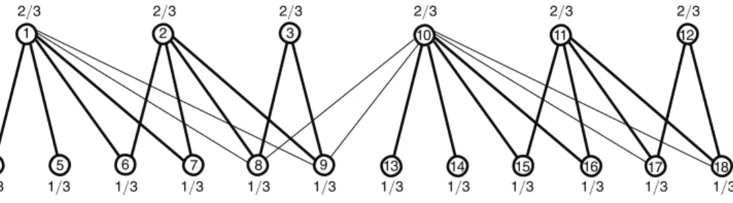
The following description of the equilibria for two simple networks illustrates the conclusions of Theorem 1. Equilibria for more complex networks are analyzed in Example 2. The uniform matching technology for the network g, deployed in
Examples 1–3, is defined by p ij= 1/e, ∀ij ∈ g where e denotes the total number of
links in g.
Example 1: Consider the network g 1 illustrated in Figure 2. The equilibrium
pay-offs in the game Γ δ played on the network g 1 , with the uniform matching
technol-ogy, are v 1* δ = ___ 150 − 250δ + 103 δ 2 5(100 − 220δ + 158 δ 2 − 37 δ 3) v 2* δ = 100 − 160δ + 63 δ 2 ___ 5 (100 − 220δ + 158 δ 2 − 37 δ 3) v 3* δ = ___ 2(25 − 40δ + 16 δ 2) 5(100 − 220δ + 158 δ 2 − 37 δ 3) v 4* δ = v 5* δ = 100 − 165δ + 67 δ 2 ___ 5 (100 − 220δ + 158 δ 2 − 37 δ 3) ,
converging to v 1* = v 2* = 3/5 and v *3 = v 4* = v 5* = 2/5 as δ → 1. There exists a unique equilibrium in which, for all ij ∈ g 1 , when i is selected to propose to j, he offers δ v j* δ , and when i has to respond to a proposal from j, he accepts any offer of at least δ v *i δ and rejects smaller offers. In equilibrium every match results in agreement.
Consider next the network g 2 , also illustrated in Figure 2. When players have
discount factor δ ≤ 10(9 − √ _2 )/79 ≈ 0.9602 ≕ _ δ , the equilibrium payoffs in the
bargaining game on the network g 2 , with the uniform matching technology, are
v 1* δ = 300 − 520δ + 223 δ 2 ___ 5 (200 − 460δ + 346 δ 2 − 85 δ 3) v 2* δ = 100 − 160δ + 63 δ 2 ___ 5 (200 − 460δ + 346 δ 2 − 85 δ 3) v 3* δ = v 4* δ = 2(50 − 85δ + 36 δ 2 ) ___ 5 (200 − 460δ + 346 δ 2 − 85 δ 3) v 5* δ = ___ 2(100 − 170δ + 71 δ 2) 5(200 − 460δ + 346 δ 2 − 85 δ 3) .
For δ ≤ δ _ , there is a unique equilibrium with a description similar to the case of g 1 .
A payoff irrelevant equilibrium multiplicity arises for the discount factor δ _ . For
δ = δ _ , it is true that δ( v 1* δ + v 5* δ ) = 1. Any behavior of player 1 in interactions with player 5 satisfying the following conditions is part of an equilibrium. Player 1’s offer
is an arbitrary probability distribution over [ 0, δ v 5* δ ]. Player 1 rejects offers smaller than δ v 1* δ , accepts with some arbitrary probability an offer of δ v
1
*δ , and accepts with
probability 1 larger offers.9
The equilibrium payoffs when δ > δ _ are
v *1 δ = _ 10 − 7δ 2 , v 3* δ = v *4δ = _ 10 − 7δ 1 , v 2* δ = v 5* δ = _ 2(5 − 4δ) 1 , converging to v 1* = 2/3, v 3 * = v 4 * = 1/3, and v 2 * = v 5 * = 1/2 as δ → 1. For δ > δ _ , in
every equilibrium agreement obtains across all links except (1, 5). The equilibrium
requirements do not pin down the disagreement offer in an encounter between play-ers 1 and 5, and there exist multiple payoff equivalent equilibria as explained in Remark 1. However, in every equilibrium, the strategies for bargaining across the
links (1, 3), (1, 4), (2, 5) must be as specified in Remark 1.
We call ( v i* δ )
i∈n the equilibrium payoff vector at δ. The equilibrium
agree-ment network at δ, denoted g *δ , is defined as the subnetwork of g with the link
ij included if and only if δ( v i* δ + v j
*δ ) ≤ 1. Hence the equilibrium agreement
net-work consists of all links where the two players at the endpoints can come up with a division of the surplus that makes both weakly better off than proceeding without agreement to the next period. For δ such that δ( v i* δ + v j* δ ) ≠ 1, ∀ij ∈ g, the agreements and disagreements in any subgame across all equilibria are
entirely characterized as in the second part of Theorem 1. Across a link ij ∈ g *δ , if
δ( v i* δ + v j* δ ) < 1 then agreement is reached with probability 1 in any equilibrium; if δ( v i* δ + v j* δ ) = 1 then there exist equilibria in which agreement is reached with
any probability. For links ij ∉ g *δ , disagreement arises with probability 1 in any
equilibrium. We show that the condition δ( v i* δ + v j* δ ) ≠ 1, ∀ij ∈ g holds for all
but a finite set of discount factors δ, hence the description of equilibrium
agree-ments and disagreeagree-ments provided by Theorem 1 is complete for generic discount factors.
PROPOSITION 1: The condition δ( v i* δ + v
j
*δ ) ≠ 1, ∀ij ∈ g holds for all but a finite
set of δ.
The proof appears in the Appendix. We outline the approach here since some of
its elements resurface in the proof of the next result. For every δ ∈ (0, 1) and every
subnetwork H of g, consider the n × n system of linear equations
(3) vi =
(
1 −∑
{ j|ij∈H} _ p ij 2)
δ v i +∑
{ j|ij∈H} _ p ij 2 (1 − δ v j), ∀i = _ 1, n .9 Note that the probability of agreement between 1
τ and 5τ ′ does not influence their own payoffs, but affects the length of time that future players of types 1 and 5 need to wait before entering the game. However, the equilibrium payoffs of future players are not affected by the induced delay since, as already mentioned, a player’s payoff is evaluated by discounting relative to his entry into the game rather than period 0.
We have shown above that v *δ solves the system for H = g *δ . It is easy to check that the system (3) has a unique solution v δ, H. In particular, v *δ = v δ, g *δ .
All entries in the augmented matrix of the linear system (3) are linear functions
of δ. Then for each i ∈ n, the solution v iδ, H is given by Cramer’s rule, as the ratio of
two determinants that are polynomials in δ of degree at most n,
v iδ, H = P iH (δ)/ Q i H(δ).
We can then argue that every δ for which there exist ij ∈ g with δ( v i* δ + v j
*δ ) = 1 is
a root of one of a finite family of nonzero polynomials in δ.
Denote by Δ the finite set of δ for which there exists ij ∈ g with
δ( v i* δ + v j* δ ) = 1. As established by Theorem 1, for δ ∉ Δ, in every equilibrium of Γ δ , in any subgame where i τ is chosen to make an offer to j τ ′ , with probability one: (1) if ij ∈ g *δ then i
τ offers δ v j* δ and j τ ′ accepts; (2) if ij ∉ g *δ then i τ makes an offer that j τ ′ rejects.
The following result establishes convergence of the equilibrium outcomes as players become patient. The proof appears in the Appendix.
THEOREM 2: There exist _ δ ∈ (0, 1) and a subnetwork g * of g such that the
equi-librium agreement network g *δ is equal to g * for all δ > δ _ . The equilibrium payoff
vector v *δ converges to a vector v * as δ goes to 1. The rate of convergence of v *δ to
v * is o(1 − δ).
We call g * the limit equilibrium agreement network and v * the limit
equilib-rium payoff vector. Our main objective is to determine the limit equilibequilib-rium
pay-offs.10 The following preliminary observations are proven in the Appendix.
PROPOSITION 2: if ij ∈ g, then v i* + v j* ≥ 1. if ij ∈ g * , then v i* + v j* = 1. in
par-ticular, if v i* + v
j
* > 1, then ij ∉ g *.
LEMMA 1: Every player has at least one link in g *(under the assumption in
foot-note 5).
REMARK 2: The benchmark model assumes that all agreements generate the
same surplus. The bargaining protocol specifies that in every match both players
are equally likely to be chosen as the proposer. However, the results of this section
generalize without difficulty to a setting with heterogenous link values and
arbi-trary asymmetric probabilities of recognizing the proposer conditional on every
link selection.
10 One can approximate the equilibrium payoffs for a given discount factor δ by iterating the contraction f δ on any initial payoff vector until convergence to its fixed point is obtained. Note that the contraction factor is δ. This computational approach can be used to determine the payoffs in any given network. However, we seek to provide a conceptual characterization of bargaining power in arbitrary networks.
IV. Bounds for Limit Equilibrium Payoffs
In order to characterize the limit equilibrium payoffs, we need to introduce
sev-eral new concepts. For every network H and subset of vertices M, let L H(M) denote
the set of players who have H-links to players in M, LH(M) = {j | ij ∈ H, i ∈ M}. A
set M is H-independent if there exists no H-link between two players in M, M ∩
L H(M) = ∅. A nonempty set of players is mutually estranged if it is g *
-indepen-dent. The set of partners for a mutually estranged set M is defined as L g *
(M).11 Fix a mutually estranged set M with partner set L. Basically, as players become patient, the set L spans the relevant bargaining opportunities of the set M. For high discount factors, since the players in M can reach equilibrium agreements only when matched to bargain with players in L, the set M is weak if L is relatively small. This intuition is formalized by the shortage ratio of M, defined as the ratio of the number
of partners to estranged players, | L |/| M |. The shortage ratio measures the collective
strength of the mutually estranged players in a sense made precise by Theorems 3 and 4.
The next result is essential for developing a procedure to determine the limit equi-librium payoffs. For every mutually estranged set M with partner set L, the ratio of the limit equilibrium payoffs of the worst-off estranged player, min i∈M v i* , and the best-off partner, max j∈L v j* , is not larger than the shortage ratio of M.
THEOREM 3: For every mutually estranged set M with partner set L, the following
bounds on limit equilibrium payoffs hold:
min i∈M v i* ≤ _ | M | + | L | | L | max j∈L v j * ≥ _ | M | | M | + | L | .
The proof of Theorem 3 is relegated to the Appendix. It uses the following result,
which follows immediately from rearranging equation (1) (with the substitution
˜
v = v *δ ).
LEMMA 2: For every δ, the equilibrium payoff of each player in Γ δ is equal to the
expected present value of his stream of first mover advantage, i.e., v i* δ = 1 _
1 − δ { j|ij∈g}
∑
_ p ij
2 max(1 − δ v i* δ − δ v j* δ , 0), ∀i ∈ n, ∀δ ∈ (0, 1). We say that max(1 − δ v i* δ − δ v j* δ , 0) measures the first mover advantage that i gains from making an offer to j. Indeed, as argued in Section III, the expected
pay-11 To illustrate the definitions, note that the list of all mutually estranged sets and corresponding partner sets in the limit equilibrium agreement network for the bargaining game on the network g 2 (Figure 2) is ({1}, {3, 4}), ({2}, {5}), ({3}, {1}), ({4}, {1}), ({5}, {2}), ({1, 2}, {3, 4, 5}), ({1, 5}, {2, 3, 4}), ({2, 3}, {1, 5}), ({2, 4}, {1, 5}), ({3, 4}, {1}), ({3, 5}, {1, 2}), ({4, 5}, {1, 2}), ({2, 3, 4}, {1, 5}), and ({3, 4, 5}, {1, 2}).
off of i is δ v i* δ in any subgame following nature’s move where he is not the proposer and max(1 − δ v j* δ , δ v
i
*δ ) in any subgame where he is selected to make an offer to
player j. Hence player i’s net benefit from getting the opportunity to make an offer to j is the difference max(1 − δ v j* δ , δ v
i *δ ) − δ v i *δ = max(1 − δ v i *δ − δ v j *δ , 0).
The intuition for the proof of Theorem 3 is as follows. Suppose that M is a mutu-ally estranged set with partner set L. Fix a discount factor δ > δ _ , with δ _ specified as
in Theorem 2. Thus, g *δ = g * . In every equilibrium, in any subgame, each player i
in M reaches agreements only with players in L with whom he shares g * links. Any
first mover advantage that a player i in M gains from making an offer to a player
j in L is mapped to an equal first mover advantage that j gains from making an
offer to i (max(1 − δ v i* δ − δ v j* δ , 0) is symmetric in i and j). Moreover, both gains are
weighted by the same probability, p ij/2, in the expected payoffs of i and j since the
two players are equally likely to make offers when matched to bargain. It follows that the sum of the expected present values of the streams of first mover advantage enjoyed by all players in M is not larger than the same expression evaluated for the
players in L.12 Hence, by Lemma 2, ∑
j∈L v j* δ ≥ ∑ i∈M v i* δ . Note that the symmetry
of the bargaining protocol is essential for this conclusion. Taking the limit δ → 1
we obtain that ∑ j∈L v j* ≥ ∑
i∈M v i* . Then the proof is made complete by repeatedly using Proposition 2 to establish that min i∈M v i* + max j∈L v j* = 1.
While Theorem 3 invokes knowledge we do not have a priori about the limit
equilibrium agreement network g * , it has an immediate corollary that exclusively
involves properties of g.13 It is sufficient to note that since g * is a subnetwork of
g, if M is g-independent then M is also g * -independent, and L g *
(M) ⊂ L g(M), so | L g *
(M) | ≤ | L g(M) |.
COROLLARY 1: For every g-independent set of players M, the following bounds
on limit equilibrium payoffs hold:
min i∈M v i* ≤ | L g (M) | __ | M | + | L g(M) | max j∈ L g(M) v j * ≥ __ | M | | M | + | L g(M) | .
V. Limit Equilibrium Payoff Computation
Theorem 3 suggests that it may be useful to study the mutually estranged sets M that minimize the upper bound | L g *
(M) |/(| M | + | L g *
(M) |) for the limit equilib-rium payoff of the worst-off player in M or, equivalently, minimize the shortage ratio | L g *
(M) |/| M |. The next lemma—applied to the network g * —shows that the set
of such minimizers is closed with respect to unions if the attained minimum is less than 1. It is useful to generalize this conclusion to all networks. The proof is in the 12 Players in M gain first mover advantage only from players in L, while players in L gain first mover advantage from the corresponding players in M, and possibly from players outside M.
Appendix. For every network H, let (H) denote the set of nonempty H-independent sets.
LEMMA 3: Let H be a network. Suppose that min M∈(H) | L H (M) | _ | M | < 1,
and that M′ and M″ are two H-independent sets achieving the minimum. Then
M′ ∪ M″ is also H-independent and
M′ ∪ M″ ∈ arg min
M∈(H) |
L H
(M) |
_ | M | .
We show that the bounds on limit equilibrium payoffs corresponding to a set of mutually estranged players and their partners provided by Theorem 3 need to be binding unless the worst-off estranged player is part of an even weaker mutually estranged set, and the best-off partner is part of an even stronger partner set. The intuition is that each player is part of a limit equilibrium oligopoly subnetwork
where, as δ → 1, some mutually estranged players and their partners share the
unit surplus according to the shortage ratio. Consequently, the limit payoff of any player cannot be smaller than the upper bound for the worst-off player from a mutually estranged set with the lowest shortage ratio. Therefore, the bounds for the limit equilibrium payoffs of the worst-off estranged player and the best-off partner corresponding to a mutually estranged set with the lowest shortage ratio must be binding.
Suppose that the lowest shortage ratio, r 1 = min M∈(g) | L g(M) |/| M |, is smaller
than 1. Let M 1 be the union of all g-independent sets M minimizing the shortage
ratio. By Lemma 3, M 1 is also a g-independent set with minimal shortage ratio. Let
L1 = L g( M 1) be the corresponding set of partners.
REMARK 3: note that g * is a priori unknown. our analysis is self-contained in
that it does not directly involve g * . Many steps in the proof of Theorem 4 below
uncover properties of g * that enable the application of Theorem 3. in particular,
we show that the lowest shortage ratio—when smaller than 1—may be computed
by restricting attention to sets that are g-independent rather than g * -independent.
Another key finding is that L g *
( M 1) = L g( M 1). Therefore, we legitimately refer to
M 1 as the largest mutually estranged set minimizing the shortage ratio, to L 1 as the
partner set of M 1 , and to r 1 as the shortage ratio of M 1 . We have argued above that min i∈ M 1 v i* = r
1/( r 1 + 1) and max j∈ L 1 v j* = 1/( r 1 + 1).
We set out to show that the limit equilibrium payoffs are given by r 1/( r 1 + 1) for
all players in M 1 and 1/( r 1 + 1) for all players in L 1 . That is, all players in M 1 ∪ L 1 , not only the worst-off estranged player and the best-off partner, have extremal limit payoffs. The following algorithm sequentially iterates this hypothesis in order to determine the limit equilibrium payoffs of all players.
DEFINITION 1: (Algorithm (g) = ( r s , x s , M s , L s , n s , g s ) s=1, 2, … , _ s ) Define the
sequence( r s , x s , M s , L s , n s , g s ) s recursively as follows: Let n 1 = n and g 1 = g. For
s ≥ 1, if n s = ∅ then stop. otherwise, let14
(4) r s = min
M⊂ n s , M∈ (g) | L g s
(M) |
_ |M | .
If r s≥ 1 then stop. Else, set x s= r s/(1 + r s). Let M s be the union of all minimizers
M in (4).15 Denote L
s= L g s( M s). Let n s+1 = n s\( M s ∪ L s) and g s+1 be the subnet-work of g induced by the players in n s+1 . Denote by _ s the finite step at which the
algorithm ends.16
At each step, the algorithm (g) determines the largest mutually estranged set
minimizing the shortage ratio in the subnetwork induced by the remaining
play-ers (Lemma 3), and removes the corresponding estranged players and partners.
Remark 3 is essential to the applicability of the procedure. The definition ensures
that (g) simultaneously identifies and removes all residual players with extremal
limit payoffs. Then, for high discount factors, the removed players reach agreements only among themselves in equilibrium, and the network induced by the remaining players can be analyzed independently. The algorithm terminates when all players have been removed or every g-independent set formed by the remaining players has shortage ratio greater than or equal to 1.
As an illustration, the algorithm ( g 2), for the network g 2 from the
introduc-tion, ends in _ s = 2 steps. The relevant outcomes are r 1 = 1/2, x 1 = 1/3, M 1 = {3, 4},
L1 = {1} at the first step and r 2 = 1, n 2 = {2, 5} at the second.
The next lemma, which is used in the proofs of Proposition 3 and Theorem 4
below, follows immediately from the specification of the algorithm (g). The proof
of Proposition 3 is provided in the Appendix.
LEMMA 4: (g) satisfies the following conditions for all 1 ≤ s ≤ s′ < _ s :
L g s( M
s ⋃ M s+1 ⋃ … ⋃ M s ′ ) = L s ⋃ L s+1 ⋃ … ⋃ L s ′
L g( n
s+1) ⋂ ( M 1 ⋃ M 2 ⋃ … ⋃ M s) = ∅
M s ⋃ M s+1 ⋃ … ⋃ M s ′ is g-independent.
PROPOSITION 3: The sequences ( r s ) s and ( x s ) s defined by (g) are strictly increasing. Note that the sets M 1 , L 1 , … , M _ s −1 , L _ s −1 , n _ s partition n. The limit equilibrium pay-off of each player is uniquely determined by the partition set that includes him.
14 It can be shown that each player in n
s has at least one link in g s , hence r s is well defined and positive.
15 By Lemma 3, since r
s< 1, M s is also a minimizer in (4).
16 In some cases the last step variables r _
THEOREM 4: Let ( r s , x s , M s , L s , n s , g s ) s=1, 2, … , _ s ) be the outcome of the algorithm
(g). The limit equilibrium payoffs for Γ δ as δ → 1 are given by
v i* = x s , ∀i ∈ M s , ∀s < _ s v j* = 1 − x s , ∀j ∈ L s , ∀s < _ s v k* = 1 _ 2 , ∀k ∈ n _ s . PROOF:
We prove the theorem by induction on s. Suppose we established the assertion for
all lower values, and we proceed to proving it for s (1 ≤ s ≤ _ s).17 We treat the case
s= _ s separately in the Appendix.
Let s < _ s and define x _ s= min i∈ n s v i* . Denote by
_
M s= arg min i∈ n s v i* the set of players in n s whose limit equilibrium payoffs equal _ x s and set L _ s= L g s( M _ s). We first show that _ x s= x s by arguing that _ x s≤ x s and _ x s≥ x s .
CLAIM 4.1: x _ s ≤ x s
We proceed by contradiction. Suppose that _ x s> x s . Then v j* ≥ 1 − x
s−1 > 1 −
x s> 1 − _ x s for all j in L 1 ∪ L 2 ∪ … ∪ L s−1 .18 The first inequality follows from the induction hypothesis and Proposition 3, and the second from Proposition 3. But
v i* ≥ _ x s for all i in M s . Thus, v i* + v j* > 1, ∀i ∈ M s , ∀j ∈ L 1 ∪ L 2 ∪ … ∪ L s−1 . By Proposition 2 no player i ∈ M s has g * links to players j ∈ L
1 ∪ L 2 ∪ … ∪ L s−1 , or L g * ( M s) ∩ ( L 1 ∪ L 2 ∪ … ∪ L s−1) = ∅. By Lemma 4, L g( M s) ∩ ( M 1 ∪ M 2 ∪ … ∪ M s−1) = ∅. It follows that L g *
( M s) ⊂ L g s( M s) = L s. Theorem 3 implies that min i∈ M s v i * ≤ _ | L s| | M s| + | L s| = x s , a contradiction with min i∈ n s v i* =
_
x s> x s . CLAIM 4.2: x _ s ≥ x s and v j* = 1 −
_
x s , ∀j ∈ _ L s .
We proved that _ x s≤ x s . Since r s< 1 it follows that x s< 1/2. By Proposition 2 and Claim 4.1,
v j* ≥ 1 − x _ s ≥ 1 − x s > 1/2, ∀j ∈ _ L s . Then Proposition 2 implies that _ L s is a g * -independent set.
17 The following technical detail is used in order to avoid analogous arguments proving the base case and the inductive step. Append step 0 to the algorithm, with ( r 0 , x 0 , M 0 , L 0 , n 0 , g 0) = (0, 0, ∅, ∅, n, g). Then the base case s= 0 follows trivially, and the inductive steps, s = 1, 2, … , _ s − 1, involve analogous arguments.