Practical correlations for the thermal resistance of vertical enclosed airspaces for building applications

(1)

Publisher’s version / Version de l'éditeur:

Building and Environment, 59, pp. 379-396, 2013-01-01

READ THESE TERMS AND CONDITIONS CAREFULLY BEFORE USING THIS WEBSITE.

https://nrc-publications.canada.ca/eng/copyright

Vous avez des questions? Nous pouvons vous aider. Pour communiquer directement avec un auteur, consultez la

première page de la revue dans laquelle son article a été publié afin de trouver ses coordonnées. Si vous n’arrivez pas à les repérer, communiquez avec nous à PublicationsArchive-ArchivesPublications@nrc-cnrc.gc.ca.

Questions? Contact the NRC Publications Archive team at

PublicationsArchive-ArchivesPublications@nrc-cnrc.gc.ca. If you wish to email the authors directly, please see the first page of the publication for their contact information.

NRC Publications Archive

Archives des publications du CNRC

This publication could be one of several versions: author’s original, accepted manuscript or the publisher’s version. / La version de cette publication peut être l’une des suivantes : la version prépublication de l’auteur, la version acceptée du manuscrit ou la version de l’éditeur.

For the publisher’s version, please access the DOI link below./ Pour consulter la version de l’éditeur, utilisez le lien DOI ci-dessous.

https://doi.org/10.1016/j.buildenv.2012.09.003

Access and use of this website and the material on it are subject to the Terms and Conditions set forth at

Practical correlations for the thermal resistance of vertical enclosed

airspaces for building applications

Saber, Hamed H.

https://publications-cnrc.canada.ca/fra/droits

L’accès à ce site Web et l’utilisation de son contenu sont assujettis aux conditions présentées dans le site LISEZ CES CONDITIONS ATTENTIVEMENT AVANT D’UTILISER CE SITE WEB.

NRC Publications Record / Notice d'Archives des publications de CNRC:

https://nrc-publications.canada.ca/eng/view/object/?id=47acb711-21f6-416b-a3b9-3b4cd69a71b3 https://publications-cnrc.canada.ca/fra/voir/objet/?id=47acb711-21f6-416b-a3b9-3b4cd69a71b3

(2)

Practical Correlations for the Thermal Resistance of Vertical

Enclosed Airspaces for Building Applications

Hamed H. Saber



Construction Portfolio, National Research Council Canada Bldg. M-24, 1200 Montreal Road, Ottawa, Ontario, Canada K1A 0R6

Abstract

Many parts of the building envelope contain enclosed airspaces. The thermal resistance (R-value) of an enclosed airspace depends on the emissivity of all surfaces that bound the airspace, the size and orientation of the airspace, the direction of heat transfer through the airspace, and the respective temperatures of all surfaces that define the airspace. The 2009 ASHRAE Handbook of Fundamentals (Chapter 26) provides a table that contains the R-values for an enclosed airspace. The ASHRAE table is extensively used by modellers, architects and building designers in the design of building enclosures. This table provides R-values for enclosed airspaces for different values of the thickness of the airspace, effective emittance, mean airspace temperature, and temperature differences across the airspace. The effect of the airspace aspect ratio (height/thickness of airspace) on the R-value is not included in the ASHRAE table. However, in a recent study on the R-value of reflective insulations using a numerical simulation model, it was shown that the aspect ratio of the airspace can affect the R-value of the enclosed airspace. The numerical simulation model used in this study had been benchmarked against experimental data obtained using two standard test methods: ASTM C-518 and ASTM C-1363.

In this paper, a numerical simulation study was conducted, that was based on previous work focused on enclosed airspaces, to investigate the effect of the aspect ratio on the R-value of vertical enclosed airspaces of different thicknesses and having a wide range of values for effective emittance, mean temperature, and temperature differences across the airspace. The R-values predicted from numerical simulation are compared with those provided in the ASHRAE table. Considerations were also given to investigating the potential increase in R-values of enclosed airspaces when a thin sheet is placed vertically in the middle of the airspace and whose surfaces have different values of emissivity. Finally, practical correlations are developed for determining the R-values of an enclosed airspace for future use by modellers, architects and building designers. The simplicity of these correlations suggests that these could be included in the ASHRAE Handbook of Fundamentals.

Keywords: Reflective insulation, low emissivity material, thermal modelling, R-value correlation,

airflow in enclosed airspace, heat transfer by convection, conduction and radiation.

(3)

INTRODUCTION

The design of building envelope roof and wall systems with the intent of achieving energy savings can necessarily help reduce building operating loads and thus the demand for energy over time [1, 2]. A straightforward means of reducing building operating costs is to limit heat transmission and thus energy loss through the building envelope. This evidently can be achieved by increasing the thermal resistance (R-value) of the building envelope. Reflective Insulation (RI) products are widely used in both space as well as terrestrial applications, for example, in building construction. For applications in building construction, and in accordance with installation guidelines of the Reflective Insulation Manufacturers Association International (RIMA-I) [3], RI products have at least one reflective surface facing an airspace. As well, RI products are typically being used in conjunction with mass insulation products, such as glass fibre, expanded polystyrene foam (EPS), and other similar insulation products. Reflective Insulation products can be installed in wall cavities, between ceiling and floor joists, to provide radiant energy barriers, and in metallic buildings that cannot readily accommodate loose-fill or batt-type insulations. Furthermore, RI products can be used as part of a roofing system either below the decking between rafters, within small air gaps between decking and roofing, and in air

gaps created, for example, by paneling interior masonry walls [4].

An enclosed airspace contributes to the overall thermal resistance of a system whether or not a product having a reflective surface is installed in the system. However, it is known that the presence of a reflective surface augments the thermal resistance of that airspace [5 – 13]. The contribution of the reflective insulation on the thermal performance (R-values and energy savings) of above-grade, and above- and below-grade wall systems having a Furred-Airspace Assembly (FAA) have been investigated for which the results are available in a number of publications [7, 9 – 13]. In the wall systems described in these studies, a low emissivity foil material was installed within the furred-airspace assembly.

The thermal resistances (R-values) of enclosed airspaces were calculated by many investigators (e.g. see [14 – 17]) for various orientations of airspaces and reflective boundaries by using heat transfer coefficient data that was published by Robinson et al. [15, 16, 17]. The heat transfer coefficient data were obtained from measurements of panels of different thicknesses (0.625 in to 3.375 in (15.9 mm to 85.7 mm)) using the test method described in ASTM 236-53 [18]. In those studies, the steady-state heat transmission rates were corrected for the heat transfer occurring along parallel paths between the hot and cold boundaries. Thereafter, the convective heat transfer coefficients were obtained from the data by subtracting a calculated radiative heat transfer rate from the total corrected heat transfer rate; and the radiative heat transfer was calculated using an emissivity of 0.028 for the aluminum surfaces. Generally, the value for the effective heat conductance, U-value (the reciprocal of the R-value), of an enclosed space (e.g. airspace) between two parallel planes depends on the physical properties of the gas, the temperature and emissivity of all the surfaces of the space, temperature differences across the space, the dimensions of the space, the direction of heat transfer through the space and the orientation of the space. The U-value accounts for the contribution of heat transfer in the enclosed space due to heat transfer by conduction, convection and radiation.

In the absence of heat transfer by radiation, the contribution of heat transfer due to convection in an enclosed space is normally given in terms of the Nusselt number, Nu (Nu = h /, where h

(4)

is convective heat transfer coefficient,  is the thickness of the space, and  is the thermal conductivity of the fluid filling the space). According to many authors [19, 20], the convective heat transfer coefficient for an enclosed space can be given as:



.

Pr



 

,

and

/

.

/







2



3



2



a

Gr

A

a

Ra

A

Gr

g

T

h

Nu



b c_R



b _Rc





(1)

Where the coefficients a, b and c in Eq. (1) are dimensionless constants, derived from

experiments, AR is the aspect ratio of the enclosed space (AR = height (H)/thickness ()), Gr is

the Grashoff number, Ra is the Raleigh number (Ra = Gr.Pr), and Pr is the Prandtl number. In order to derive the coefficients a, b and c (Eq. (1)), from which the heat transfer coefficient, h, due to the convective component of heat transfer can be determined, the emissivity of all surfaces that bound the enclosed space must be zero (i.e. purely reflective surfaces). However, it is not possible in practice, to use materials having zero emissivity when conducting such experiments. Hence, to derive the coefficients a, b and c of Eq. (1) from experiments, as mentioned previously, the rate of radiative heat transfer across the enclosed space would be subtracted from the total rate of heat transfer across the space.

A number of correlations for the value of Nu in the form of the relationship given in Eq. (1) and

for different ranges of values of Ra, AR and Pr are provided in several studies as described in

the IEA Annex XII report [19]. Some of these correlations showed the dependence of the Nu on

the aspect ratio of the enclosed space (AR). As such, it is anticipated that the effective thermal

conductance or the effective thermal resistance of the enclosed space would be affected by the aspect ratio of the space, as will be shown later in this study.

Yarbrough [4] developed a one-dimensional, steady-state model, called “REFLECT” to provide R-values of reflective assemblies and the model was further used to help establish the sensitivity of R-values to the values of surface emissivity and as well, the location of foil surfaces inside an enclosed airspace. The model was used to calculate the R-values using the heat transfer coefficients derived by Robinson [15, 16, 17] combined with a term accounting for repeated reflection of energy between infinite parallel planes based on the Stefan-Boltzmann law. The R-values obtained using the REFLECT model are thus independent of the aspect ratio of the enclosed airspace [4].

The 2009 ASHRAE Handbook of Fundamentals (Chapter 26) [14] provides a table that contains the R-values for an enclosed airspace and these were determined on the basis of the heat transfer data reported by Robinson et al. [15, 16, 17]. These values were obtained by combining the convective and radiative components of heat transfer from which the total thermal resistance value for an enclosed airspace was provided for airspaces of different thickness ( =

13, 20, 40, and 90 mm), mean temperature (Tavg= 32.2, 10.0, -17.8 and -45.6oC), temperature

difference across the airspace (T = 5.6, 11.1 and 16.7o_{C), effective emittance (}

eff= 0.03, 0.05,

0.2, 0.5 and 0.82), and direction of heat flow through the airspace. Note that the effective

emittance (εeff) of an enclosed airspace is given as [14]:

, 1 / 1 / 1 / 1



_eff 



₁



₂ (2)

where



₁ and



₂ are the emissivity of the hot and cold surfaces.

The ASHRAE table [14] is being used extensively by modellers, architects and building

designers. The R-value of an enclosed airspace at other values of the parameters , eff, Tavg,

(5)

the effect of the aspect ratio of the enclosed airspace on the R-value is likewise not included in this ASHRAE table [14].

MODEL DESCRIPTIONS AND BENCHMARKING

The NRC’s hygrothermal model “hygIRC-C” was used in this study to predict the R-values of

vertical enclosed airspaces having different eff and subjected to wide ranges of Tavg and T.

This model solves simultaneously the 2D and 3D moisture transport equation, the energy equation, the surface-to-surface radiation equation (e.g. the surface-to-surface radiation in the enclosed airspace, an example is provided in Figure 1) and the air transport equation in the various material layers. The air transport equation is the Navier-Stokes equation for the

airspace layers (e.g. air cavities), and the Darcy equation (Darcy Number, DN <10-6_{) and}

Brinkman equation (DN > 10-6_{) for the porous material layers. The present model was}

benchmarked [27] against the hygIRC-2D model previously developed at NRC [28, 29], and against experimental results from the evaluation of a number of different wall assemblies. A full description of the present model is available in previous publications (see references [1-2, 6-13, 24-27]).

In building applications that are similar to this study, the present model was benchmarked against thermal performance data for a wall assembly featuring a reflective insulation product. The data was obtained using a Guarded Hot Gox (GHB) (in accordance with ASTM C-1363 test method [21]) for a full-scale (8 ft x 8 ft) above-grade wall system. This wall featured 2 x 6 wood framing, stud cavities filled with friction-fit glass fiber batt insulation, and a layer of foil-lined fiberboard installed to the interior side of the framing, with the foil facing a furred-airspace. Results showed that the R-value predicted by the model for this wall system was in good agreement with the measured R-value (within 1.2%) [11, 22].

Recently, a number of tests were conducted at the Cold Climate Housing Research Center

(CCHRC) [5] and the NRC [6, 8] that examined the thermal performance of different types of

reflective insulations. The tests were conducted using a Heat Flow Meter, HFM (in accordance with ASTM C-518 test method [23]) capable of accommodating product samples with maximum dimensions of 12 in x 12 in x 4 in (length x width x thickness). In these tests, sample stacks including different types of reflective insulations were placed horizontally between the upper cold plate and lower hot plate of the heat flow meter (i.e. upward heat flow). Each sample stack consisted of three layers. The upper layer (12 in x 12 in x 1 or 2 in) was made of reflective insulation (foil adhered to the bottom surface). The bottom layer was made of gypsum (12 in x

12 in x ½ in) [5] or EPS (12 in x 12 in x 1 in) [6, 8]. To quantify the thermal resistance

contribution of the reflective insulation component, an air cavity (8 in x 8 in x 1 in) was created in the center of an EPS layer (12 in x 12 in x 1 in), which was placed between the reflective layer and the bottom layer. As shown in references [6, 8], the heat fluxes predicted by the model

were in good agreement with all measured heat fluxes from these tests (within 1.0%).

Thereafter, the model was used to investigate the contribution of reflective insulations to the R-value for specimens with different inclination angles, different directions of heat flow through the specimens, and a wide range of foil emissivity [6].

In the study [6], the prediction of the R-values using the model described above was compared with the R-values given in the ASHRAE table [14] for an enclosed airspace having a thickness of 20 mm. As previously indicated, the effect of the aspect ratio of the airspace is not accounted for on the basis of the R-values given in the ASHRAE table [14]. Given that in conducting a

(6)

numerical simulation, the length of the enclosed airspace is required to define the computational domain, a sensitivity analysis was conducted in the study [6] to investigate its effect on the R-value. Three airspace lengths were considered in this analysis: 4 in (101.6 mm), 8 in (203.2 mm) and 16 in (406.4 mm). For a horizontal airspace of different lengths and in the case of

upward heat flow when eff= 0.05, Tavg= 32.2oC, T = 5.6oC, results showed that the R-value

depended on the length of the airspace. For example, increasing the airspace length from 4 in (101.6 mm) to 8 in (203.2 mm) and from 4 in (101.6 mm) to 16 in (406.4 mm) resulted in an increase in its value of 1.5% and 3.7%, respectively. Furthermore, results showed that the R-value from the ASHRAE table [14] was 14.8%, 13.0% and 10.7% greater than the R-R-value predicted by the model for respective airspace lengths of 4 in (101.6 mm), 8 in (203.2 mm) and 16 in (406.4 mm). For an airspace with a length of 8 in (203.2 mm), and for which the value of

effective emittance (eff) ranged between 0.5 and 0.82 (high value range), the corresponding

R-values predicted by the model and taken from the ASHRAE table [14] were in good agreement

(within  ±3.5%). Whereas, for low values of effective emittance (eff), the R-values obtained

from the ASHRAE table [14] were, respectively, 14.0%, 13.0% and 6.1% greater than that

predicted by the model for values of eff= 0.03, 0.05 and 0.2. The results obtained for the low

emissivity values are in agreement with those of a recent study by Craven and Garber-Slaght [5]. In this study [5] it was shown that the R-values taken from the ASHRAE table [14] were also greater than R-values measured in the case of low emissivity materials.

The effects of the inclination angle and the direction of heat flow through an enclosed airspace (20 mm thick, 8 in (203.2 mm) long) were also investigated and thereafter a comparison was made of the R- values predicted by the model to those obtained from the ASHRAE table [14]. A

series of comparisons was undertaken for an airspace subjected to Tavg= 32.2oC, T = 5.6oC for

the following five cases [6]:

 Case I: horizontal airspace ( = 0o_{) with upward heat flow;}

 Case II: inclined airspace ( = 45o_{) with upward heat flow;}

 Case III: vertical airspace ( = 90o_{) with horizontal heat flow;}

 Case IV: inclined airspace ( = 45o_{) with downward heat flow, and;}

 Case V: horizontal airspace ( = 0o_{) with downward heat flow.}

The results of these comparison cases showed that for Case II and Case V, the R-values predicted by the model and those given in the ASHRAE tables [14] were in good agreement for

all values of eff(within  ±6.3%). For Case III and Case IV, the R-values predicted by the model

and given in the ASHRAE tables [14] were in good agreement (within  ±2.0%) for high values

of eff (0.5 and 0.82). Whereas in Case III at low values of eff, the R-values obtained from the

ASHRAE table [14] were 24.9%, 21.7% and 12.7% higher than those predicted by the model for

eff= 0.03, 0.05 and 0.2, respectively. Also, in Case IV for low values of eff, the R-values given

in the ASHRAE table [14] were 16.5%, 16.1% and 7.7% greater than those predicted by the

model for eff= 0.03, 0.05 and 0.2, respectively (see [6] for more details).

In this paper, numerical simulations were conducted to predict the R-values of enclosed vertical airspaces. The results of the numerical simulations described in this paper follow on the work of a previous study [6] and in addition provide results for vertical enclosed airspaces (Case III)

subjected to different mean temperatures (Tavg) and temperature differences (T) across the

(7)

 Investigate the effect of the aspect ratio (AR) on the R-value of enclosed airspaces of different thicknesses ( = 13, 20, 40 and 90 mm) for a wide range of effective emittance

values (eff= 0 – 0.82).

 Compare the R-values predicted by the model and those given in ASHRAE [14] for

airspaces having different values for , Tavg, T, and eff.

 Develop practical correlations for the R-values of enclosed airspaces covering a wide

range of values for AR, Tavg, T, and efffor subsequent use in currently available energy

simulation models (e.g. ESP-r, Energy Plus, DOE).

 Investigate the potential increase in the R-value of an enclosed airspace when a thin sheet having an emissivity ranging between 0.0 to 0.9 is placed vertically in the middle of the airspace.

RESULTS AND DISCUSSIONS

Numerical simulations were conducted in order to predict the effective thermal resistances (R-values) of vertical enclosed airspaces for the same parameters listed in ASHRAE table [14]: (a)

thickness ( = 13, 20, 40 and 90 mm), (b) mean temperature (Tavg = 32.2, 10.0, 17.8 and

-45.6o_{C), (c) temperature difference across the airspace (T = 5.6, 11.1 and 16.7}o_{C), and (d)}

effective emittance (eff= 0 – 0.82). In order to quantify the effect of the aspect ratio (AR= H/)

of the enclosed airspace on the R-values, for a given airspace thickness (), the numerical simulations were conducted at different heights (H = 8 – 96 in (203.2 – 2438.4 mm)). The purpose of considering a wide range of values for H was to permit the development of practical correlations for determining R-values that cover most of expected building applications having vertical enclosed airspaces. These applications include, for example: double glazed windows and curtain walls of different heights, and Furred-Airspace Assemblies (FAA) attached to thermal insulation (bonded by Low Emissivity Material, LEM) in wall systems having horizontal furring and vertical furring of different center-to-center spacing [6 – 13].

A schematic is shown in Figure 1a of a vertical enclosed airspace in which only one vertical

surface of the airspace has a low value of emissivity (1), and all other surfaces have a high

value of emissivity (2). This represents, for example, the case of low-e coating of a double

glazed window or thermal insulation bonded by LEM (e.g. aluminum foil) that faces the enclosed airspace. Note that the value of the low emissivity surface can increase in the case where, for example, the surface accumulates dust (see the study by Cook et al. [30] for more details) or vapor condenses on this surface.

Most construction materials have an emissivity of 0.9 [14]. In this study, the numerical

simulations were conducted for different values of 1 (ranging from 0 – 0.9) and 2was taken

equal to 0.9. According to Eq. (2), a wide range of the effective emittance, eff(ranging from 0 –

0.82) was considered. Note that eff = 0.82 represents the case when all surfaces of the

enclosed airspace have an emissivity of 0.9 (i.e. no LEM installed on the surfaces of the enclosed airspace).

For an enclosed airspace with H = 12 in (304.8 mm), numerical simulations were also conducted in order to investigate the potential increase in R-values of the enclosed airspace

when a thin sheet (0.1 mm thick) of sides having low emissivity (1), is placed vertically in the

middle of the airspace (see Figure 1b). The thin sheet divides the enclosed airspace into two cavities of equal thickness. It was assumed that no cross airflow occurs between the two cavities (i.e. each cavity is treated as a sealed airspace). The numerical simulations were

(8)

conducted for a wide range of values for , 1, 2, Tavg, and T. In this paper, the simulation case for which there is no thin sheet material in the airspace is referred to as “1-Cavity” (Figure 1a), whereas “2-Cavities” refers to the case with a thin sheet in the airspace (Figure 1b).

Comparisons between Simulation Cases “1-Cavity” and “2-Cavities”

As indicted earlier, the modes of heat transfer in the enclosed airspace occur by conduction, convection, and radiation. Figure 2 through Figure 5 show the temperature and vertical velocity

contours in the enclosed airspace (H = 12 in (304.8 mm)) with different values of  for the

simulation cases that relate to “1-Cavity” and “2-Cavities” when Tavg= 10oC, T = 16.7oC (TH =

18.35o_{C and T}

C= 1.65oC), 1= 0.05, and 2 = 0.9. Note that different scales were used for the

vertical velocity contours in Figure 2b through Figure 5b for simulation cases “1-Cavity” and “2-Cavities”.

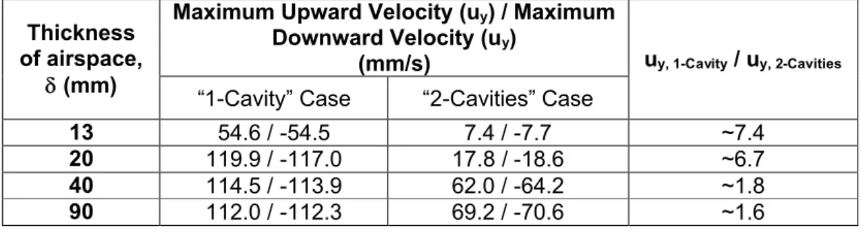
Owing to the temperature differential across the enclosed airspace, a buoyancy-driven flow developed within the airspace. A mono-cellular airflow (one convection loop) is developed within each enclosed airspace for the cases of “1-Cavity” and “2-Cavities”. As shown in Figure 2b through Figure 5b, the vertical air velocities for the “1-Cavity” simulation case are significantly higher than that for the “2-Cavities” case, resulting in a stronger convection current with one convection loop for the “1-Cavity” as compared to the “2-Cavities” case for which there was one convection loop in each cavity. Consequently, the rate of heat transfer by convection for the “1-Cavity” case is greater than that of the “2-Cavities” case resulting in higher thermal conductance (i.e. lower thermal resistance) in the “1-Cavity” as compared to the “2-Cavities” case, as shown in Figure 6 through Figure 9.

The values of the maximum upward (+ve) and downward (-ve) vertical velocities (uy) taken from

Figure 2b through Figure 5b are summarized in Table 1 for “1-Cavity” and “2-Cavities” simulation cases at different airspace thicknesses ranging between 13 mm and 90 mm. These values indicate that the vertical upward or downward velocities in the airspace are greater for the “1-Cavity” as compared to the “2-Cavities” case, ranging by a factor of 7.4 at the smallest thickness (13 mm) to 1.6 at the largest airspace thickness (90 mm).

For enclosed airspace of  = 13, 20, 40 and 90 mm (H = 12 in (304.8 mm)) at different eff, Tavg

and T, comparisons between the R-values for the cases of “1-Cavity” and “2-Cavities” are

shown in Figure 6 through Figure 9. As shown in these figures, the R-values for the “2-Cavities” simulation case are higher than that of the “1-Cavity” case. As shown Table 2, the increase in the R-value due to the incorporation of a thin sheet in the middle of the enclosed airspace (see

Figure 1b) and having an emissivity = 1 on both sides of the thin sheet, increases as 

increases from 13 mm to 20 mm and 40 mm. This percentage increase in the R-value was approximately the same by further increasing  from 40 mm to 90 mm. For example, depending

on the values of Tavgand T, the percentage increase in the R-value for eff= 0.03 changes: (a)

from 10.6% to 34.4% for  = 13 mm, (b) from 29.8% to 100.0% for  = 20 mm, (c) from 120.3 to

136.9% for  = 40 mm, and (d) from 116.8 to 128.6 for  = 90 mm (Table 2). Similarly, for eff=

0.82, the percentage increase in the R-value changes: (a) from 48.8% to 59.4% for  = 13 mm,

(b) from 72% to 98.3% for  = 20 mm, (c) from 103.0 to 113.7% for  = 40 mm, and (d) from

97.8 to 102.7 for  = 90 mm (Table 2). In summary, the R-value could be doubled due to

installing a thin sheet in the middle of the enclosed airspace. The results presented in this section could be important for future applications when a thin reflecting foil is placed in the middle of the airspace of double glazed windows and curtain wall systems so as to enhance the energy performance of these systems.

(9)

Comparison between R-values Predicted by model and Listed in

ASHRAE Table [14]

For an enclosed airspace of H = 12 in (304.8 mm) and different airspace thicknesses ( = 13, 20, 40 and 90 mm), Figure 6 through Figure 9 show the dependence of the R-value on the

effective emittance, eff, for the “1-Cavity” and “2-Cavities” simulation cases when the enclosed

airspace was subjected to different values of Tavg, and T. For the purpose of comparison, the

R-values from the 2009 ASHRAE table (eff= 0.03, 0.05, 0.2, 0.5, 0.82) [14], which correspond

to the predicted R-values for the “1-Cavity” simulation case are also shown in these figures.

For an enclosed airspace of  = 13 mm (H = 12 in (304.8 mm)) and for the “1-Cavity” case,

Figure 6 shows that the predicted R-values are in good agreement with R-values of the

ASHRAE table for all values of effwhen Tavg= 32.2oC, T = 5.6oC (Figure 6a), Tavg= 10.0oC, T

= 5.6o_{C (Figure 6c), and T}

avg= -17.8oC, T = 5.6oC (Figure 6e). For other values of Tavgand T,

the predicted R-values are in good agreement with R-values of the ASHRAE table at high eff

(0.2, 0.5 and 0.82); however, at low values of eff(0.03, 0.05), the R-values in the ASHRAE table

are greater than those predicted by the numerical model. For example, at eff = 0.03, the

R-values in the ASHRAE table are higher than the predicted R-R-values by 8.1% (Tavg= 10.0oC, T

= 16.7o_{C, Figure 6b), 8.9% (T}

avg= -17.8oC, T = 11.1oC, Figure 6d), 10.5% (Tavg= -45.6oC, T =

11.1o_{C, Figure 6f), and 6.0% (T}

avg= -45.6oC, T = 5.6oC, Figure 6g).

For an enclosed airspace of  = 20 mm (H = 12 in (304.8 mm)), it is shown in Figure 7 that the predicted R-values are in good agreement with those given in the ASHRAE table at high values

of eff(0.5 and 0.82) for all values of Tavgand T. However, at low values of eff(0.03, 0.05 and

0.2) the R-values of the ASHRAE table are higher than the predicted R-values, whereas the

difference between these values increases as eff decreases. At eff= 0.03, the R-values given

in ASHRAE are higher than the predicted R-values by 15.2% (Tavg= 32.2oC, T = 5.6oC, Figure

7a), 20.7% (Tavg = 10.0oC, T = 16.7oC, Figure 7b), 16.6% (Tavg = 10.0oC, T = 5.6oC, Figure

7c), 19.6% (Tavg= -17.8oC, T = 11.1oC, Figure 7d), 19.6% (Tavg = -17.8oC, T = 5.6oC, Figure

7e), 14.6% (Tavg = -45.6oC, T = 11.1oC, Figure 7f), and 20.1% (Tavg = -45.6oC, T = 5.6oC,

Figure 7g).

For enclosed airspace of  = 40 mm (H = 12 in (304.8 mm)), Figure 8 shows that the predicted

R-values are in good agreement with ASHRAE R-values at high values of eff(0.2, 0.5 and 0.82)

for all values of Tavg and T and at all values of efffor Tavg= -45.6oC, T = 11.1oC (Figure 8f).

At low eff (0.03, 0.05) the ASHRAE R-values are higher than the predicted R-values. At eff =

0.03, the ASHRAE R-values are higher than the predicted R-values by 37.9% (Tavg= 32.2oC, T

= 5.6o_{C, Figure 8a), 12.8% (T}

avg= 10.0oC, T = 16.7oC, Figure 8b), 30.7% (Tavg= 10.0oC, T =

5.6o_{C, Figure 8c), 11.9% (T}

avg= -17.8oC, T = 11.1oC, Figure 8d), 17.9% (Tavg= -17.8oC, T =

5.6o_{C, Figure 8e), 5.4% (T}

avg= -45.6oC, T = 11.1oC, Figure 8f), and 13.2% (Tavg= -45.6oC, T

= 5.6o_{C, Figure 8g).}

Similarly, for an enclosed airspace of,  = 90 mm (H = 12 in (304.8 mm)), Figure 9 shows that

the predicted R-values are in good agreement with ASHRAE R-values at high eff(0.2, 0.5 and

0.82) for all values of Tavg and T. At low values of eff(0.03, 0.05) the ASHRAE R-values are

higher than the predicted R-values. At eff = 0.03, the ASHRAE R-values are higher than the

(10)

16.7o_{C, Figure 9b), 25.3% (T}

avg = 10.0oC, T = 5.6oC, Figure 9c), 14.9% (Tavg = -17.8oC, T =

11.1o_{C, Figure 9d), 17.7% (T}

avg = -17.8oC, T = 5.6oC, Figure 9e), 12.6% (Tavg= -45.6oC, T =

11.1o_{C, Figure 9f), and 15.2% (T}

avg= -45.6oC, T = 5.6oC, Figure 9g).

In summary, for enclosed airspaces of height of 12 in (304.8 mm) and different thicknesses, the R-values from ASHRAE are in good agreement with the predicted R-values derived from

numerical simulation at high values of eff (0.5 and 0.82). However, at low values of eff (0.03,

0.05 and 0.2) the ASHRAE R-values are higher than the predicted R-values.

Dependence of the R-value on the Aspect Ratio

For enclosed airspaces of different thickness ( = 13, 20, 40 and 90 mm), numerical simulations

were conducted at Tavg = 32.2, 10.0, -17.8 and -45.6oC, T = 5.6, 11.1 and 16.7oC, eff = 0 –

0.82, and different aspect ratios, AR (AR = H/, H = 8 – 96 in (203.2 – 2,438.4 mm)). The

R-values obtained from the results of the simulation are shown in Figure 10 through Figure 13. Because the predicted R-values for enclosed airspaces ( = 13 mm, Figure 10) having heights of H = 56 in (1,422.4 mm) and 88 in (2,235.2 mm) were quite close, no numerical simulations were conducted at a height of H = 96 in (2,438.4 mm). For the purpose of comparisons, these figures also show the R-values taken from the ASHRAE table [14] for different values of airspace thickness, .

In recent studies [7, 9], the contribution of Furred-Airspace Assembly (FAA) to the R-values of wall systems with horizontal furring and vertical furring of the same center-to-center spacing were investigated. The FAA was attached to EPS layer (1 in (25.4 mm) thick), which was bonded by Low Emissivity Material (LEM) facing the airspace (1 in (25.4 mm) thick). The results from these studies [7, 9] showed that the contribution of FAA to the R-value of a wall with vertical furring was greater than that for a wall with horizontal furring. Note that the height of the enclosed airspace in the wall with vertical furring was greater than that in the wall with horizontal furring. In this study, it can be determined from a review of Figure 10 to Figure 13 that the R-value of an enclosed airspace of longer height is greater than that of an enclosed airspace of shorter height. For example, in Figure 10b for an enclosed airspace having a thickness of 13

mm (Tavg= 10.0oC, T = 16.7oC), it is shown that increasing H from 8 in (203.2 mm) (AR= 16) to

88 in (2,235.2 mm) (AR = 172) resulted in an increase in the R-value by 20.3% at eff = 0.03.

This observation is in agreement with results from previous studies [7, 9].

In Figure 11b, it is shown that for an enclosed airspace having a thickness of  = 20 mm eff =

0.03 (Tavg = 10.0oC, T = 16.7oC), an increase of H from 8 in (203.2 mm) (AR = 10) to 96 in

(2,438.4 mm) (AR = 122) resulted in an increase of R-value by 48.4%. Likewise as given in

Figure 12b, for enclosed airspace of  = 40 mm at eff = 0.03 (Tavg= 10.0oC, T = 16.7oC), an

increase of H from 8 in (203.2 mm) (AR = 5) to 96 in (2,438.4 mm) (AR = 61) resulted in an

increase of R-value by 86.5%. Finally, as provided in Figure 13b, for enclosed airspace of  =

90 mm at eff= 0.03 (Tavg= 10.0oC, T = 16.7oC), an increase of H from 8 (203.2 mm) in (AR= 2)

to 96 in (2,438.4 mm) (AR= 27) resulted in an increase of R-value by 84.0%.

More observations were made from results obtained by numerical simulation to derive R-values and that are shown in Figure 10 through Figure 13 are the following:

 The results cover a wide range of aspect ratios (AR) from 2 to 172 (16 to 172, 10 to 122,

(11)

 For a given value of  and eff, the increase in the R-value due to increasing the value of

aspect ratio depends on the values of Tavgand T.

 The heights of airspace that result in the closest agreement between the predicted R-values and the ASHRAE R-R-values [14] are provided in Table 3.

Practical Correlations for the R-values

The resulting R-values that were presented in the previous section for an enclosed airspace of selected thicknesses ranging between  = 13 mm to  = 90 mm, and as provided in Figure 10 to Figure 13 inclusively were used to develop practical correlations for the R-values. For the wide application of these correlations, two types of correlations were considered:

I. For given set of values for Tavg and T, as are also provided in the ASHRAE table [14], a

correlation was developed for each value of thickness, , to obtain the corresponding R-value

in (ft2_hro_{F/BTU) as a function of A}

Rand eff. This correlation is given in the following form:

. ) ( 4 1 0 1 2 3 effi i i R eff R R avg c T a A aA A b R value R  



 





      (3)

Where the coefficients

R

_c

(

T

_avg

),

a

₀

,

a

in Eq. (3) are listed in

Table 4 for different values of . In Eq. (3),

R

_c

(

T

_avg

)

is the R-value in (ft2_hro_{F/BTU) of the}

enclosed airspace due to conduction only, which also can be given as:

)

(

/

)

(

_avg _avg c

T

R







, (4) where, 15 -1E -7.4386433 11, -E 4.11702505 8, -6E -7.9025285 4, -E 1.15480022 3562, -0.0022758 , ) ( 4 3 2 1 0 4 0      



 f f f f f T f T _avgi i i avg



(5)

Note that



(

T

_avg

)

in Eq. (5) is the average thermal conductivity of air in (W/mK), which is

evaluated at the mean temperature of the airspace,

T

_avg in (K). It is important to point out that

the calculated value of R_c(T_avg) from Eq. (4) and (5) must be converted to be in (ft2_hro_{F/BTU) in}

order to be used in Eq. (3).

II. A comprehensive correlation was developed for each value of  to obtain the R-value in

(ft2_hro_{F/BTU) as a function of all parameters (i.e. T}

avg, T, AR and eff). This correlation is

(12)

 

i eff i i c a avg R c a avg eff R c a avg R avg c T a A T T aA T T A T T b R value R  



 





         4 1 0 1 1 1 2 2 2 3 3 3 ) ( (6)

In Eq. (6),

R

_c

(

T

_avg

)

is given by Eq. (4) and (5) and its unit must be in (ft2_hro_{F/BTU), whereas}

units for

T

_avg and T must be in (K). The other coefficients in Eq. (6)

, , , , , ,

(a₀ a b₁ b₂ b₃ b₄



₁,



₂,



₃,



,a₁,a₂,a₃,c₁,c₂, andc₃) are listed in Table 5. In order to

minimize the error in developing this correlation, these coefficients were obtained for values of

eff< 0.4 and eff 0.4 (see Table 5).

Note that the first term in RHS of Eq. (3) and Eq. (6) represents the R-value due to heat transfer by conduction only. The second term on the RHS of these equations represents the reduction in R-value due to heat transfer by convection only. The final two terms on the RHS of these equations represent the reduction in R-value due to heat transfer by radiation only at different

values of eff.

For an enclosed airspace of a given thickness, the predicted R-values obtained using the numerical simulation model (see Figure 10 through Figure 13) are compared with those obtained using the correlations given in Eq. (3) and Eq. (6). These comparisons are shown in Figure 14 ( = 13 mm), Figure 15 ( = 20 mm), Figure 16 ( = 40 mm), and Figure 17 ( = 90 mm). As shown in these figures, most of the predicted R-values are in good agreement with those obtained using the correlation given by Eq. (3) (within ±3%, as given in Figure 14a to Figure 17a). Furthermore, most of the predicted R-values are in good agreement with those obtained using the correlation given by Eq. (6) (within ±5%, as shown in Figure 14b to Figure 17b).

SUMMARY AND CONCLUSIONS

The numerical simulation model used in this study, had been benchmarked against experimental data derived for reflective insulations, as reported in previous studies [6, 8, 11], on the basis of results derived from two standard test methods: (i) Guarded Hot Box (GHB) in accordance with ASTM C-1363, and (ii) Heat Flow Meter (HFM) in accordance of ASTM C-518. In the first portion of this study, the model was used to conduct numerical simulations to predict the thermal resistance (R-value) of vertical enclosed airspaces of different dimensions and effective emittance. The various airspaces were subjected to different mean temperatures and temperature differences. The R-values predicted by the model were compared to those provided in the ASHRAE table [14] for the different conditions. The dependence of the R-value on the aspect ratio of the enclosed airspace was investigated for different conditions. Depending on the thickness of the enclosed airspace and the boundary conditions, the results showed that the aspect ratio can have a significant effect on the R-value (e.g. up to ~85% for an effective emittance of 0.03). Considerations were also given to investigating the potential increase in the R-value of the enclosed airspace when a thin sheet having different values of emissivity on both sides was placed vertically in the middle of the airspace. Depending on the effective emittance, the results showed that the R-value could be doubled with the incorporation of this thin sheet along the middle of the enclosed airspace.

In the second portion of this study, practical correlations were developed to determine the R-values of enclosed airspaces of different thicknesses (), and for a wide range of R-values for

(13)

various parameters, including: (a) aspect ratio (AR), (b) temperature difference across the

airspace (T), (c) mean temperature (Tavg), and, (d) effective emittance (eff). Two types of

correlations were developed:

I. For selected values of Tavgand T that are given in the ASHRAE table [14], a correlation was

developed for each value of  to obtain the R-value as a function of AR and eff. This

correlation is given by Eq. (3). The predicted R-values from the numerical model and those obtained using these correlations were in good agreement (mainly within ±3%).

II. A comprehensive correlation was developed for each value of  to obtain the R-value as a

function of Tavg, T, ARand eff. This correlation is given by Eq. (6). The predicted R-values

from the model and those obtained using this correlation agreed within ±5%.

It is of practical importance in the design of building envelopes to determine the R-value of enclosed airspaces having different values of effective emittance under varying climatic conditions to avoid selecting oversized heating and cooling equipment. The practical correlations that were developed in this paper can be used by architects and building designers to determine the R-values of vertically enclosed airspaces having varying aspect ratios and values of effective emittance, and subjected to a wide range of mean temperatures and temperature differences across the airspace. These correlations can also be readily implemented in currently available energy simulation models (e.g. ESP-r, Energy Plus, DOE, etc). Similar practical correlations for determining the R-values of flat and sloped roof applications having enclosed airspaces of different orientations and directions of heat flow will be reported in future publications.

Acknowledgments

The author thanks Dr. M. A. Lacasse, Dr. W. Maref, Ms. M. Armstrong, and Dr. A. Laouadi for their technical support.

NOMENCLATURE

AR Aspect ratio, the ratio between the height and the thickness

g Gravitational acceleration, 9.81 m/s2

Gr Grashoff number

h Convective heat transfer coefficient (W/(m2_.K))

H Height of enclosed airspace (m)

Nu Nusselt number

Pr Prandtl number

Ra Rayleigh number (Gr. Pr)

Tavg Mean temperature (K)

T Temperature difference across the enclosed airspace (K)

 Thermal expansion coefficient (1/K)

 Density of the gas (kg/m3_),

 Dynamic viscosity (Pa.s),

 Airspace thickness (m)

 Thermal conductivity (W/(m.K))

 Emissivity

(14)

REFERENCES

1. H.H. Saber, M.C. Swinton, P. Kalinger, and R.M. Paroli, “Hygrothermal Simulations of

Cool Reflective and Conventional Roofs”, 2011 NRCA International Roofing Symposium, Emerging Technologies and Roof System Performance, held in Sept. 7-9, 2011, Washington D.C., USA.

2. H.H. Saber, M.C. Swinton, P. Kalinger, and R.M. Paroli, “Long-Term Hygrothermal

Performance of White and Black Roofs in North American Climates”, Journal of Building

and Environment, 50, p. 141-154, 2012, DOI: 10.1016/j.buildenv.2011.10.022,

http://dx.doi.org/10.1016/j.buildenv.2011.10.022.

3. Reflective Insulation Manufacturers Association International (RIMA-I). Reflective

Insulation, Radiant Barriers and Radiation Control Coatings. Olathe, KS: RIMA-I, 2002.

4. D. Yarbrough, Assessment of reflective insulations for residential and commercial

applications. ORNL/TM-8891, Oak Ridge National Laboratory, Oak Ridge, TN. P. 1-63, 1983.

5. C. Craven, and R. Garber-Slaght, “Product Test: Reflective Insulation in Cold Climates”,

Technical Report Number TR 2011-01, Cold Climate Housing Research Center (CCHRC), Fairbanks, AK 99708, www.cchrc.org, April 12, 2011.

6. H.H. Saber, “Investigation of Thermal Performance of Reflective Insulations for Different

Applications, Journal of Building and Environment, 55, p. 32-44, 2012 (doi:10.1016/j.buildenv.2011.12.010).

7. H.H. Saber, and W. Maref, “Effect of Furring Orientation on Thermal Response of Wall

Systems with Low Emissivity Material and Furred-Airspace”, The Building Enclosure Science & Technology (BEST3) Conference, held in April 2-4, 2012 in Atlanta, Georgia, USA.

8. H.H. Saber, W. Maref, G. Sherrer, M.C. Swinton, “Numerical Modelling and

Experimental Investigations of Thermal Performance of Reflective Insulations”, Journal of Building Physics, The online version of this article can be found at:

http://dx.doi.org/10.1177/1744259112444021, April 26, 2012.

9. H.H. Saber, “Thermal Performance of Wall Assemblies with Low Emissivity” Journal of

Building Physics, DOI: 10.1177/1744259112450419,

http://jen.sagepub.com/content/early/2012/07/02/1744259112450419, July, 4, 2012.

10.H.H. Saber, and M.C. Swinton, “Determining through numerical modeling the effective

thermal resistance of a foundation wall system with low emissivity material and furred – airspace”, 2010 International Conference on Building Envelope Systems and Technologies, ICBEST 2010, Vancouver, British Colombia, Canada, June 27-30, 2010, pp. 247-257.

11.H.H. Saber, W. Maref, M.C. Swinton, and C. St-Onge, "Thermal analysis of above-grade

wall assembly with low emissivity materials and furred-airspace," Journal of Building and

Environment, volume 46, issue 7, pp. 1403-1414, 2011

(doi:10.1016/j.buildenv.2011.01.009).

12.H.H. Saber, W. Maref and M.C. Swinton, “Numerical investigation of thermal response of

basement wall systems with low emissivity material and furred – airspace”, 13th Canadian Conference on Building Science and Technology (13th CCBST) Conference, held in May 10 – 13, 2011 in Winnipeg, Manitoba, Canada.

13.H.H. Saber, W. Maref, and M.C. Swinton, “Thermal Response of Basement Wall

Systems with Low Emissivity Material and Furred Airspace”, Journal of Building Physics,

Published online in 5 August 2011, DOI: 10.1177/1744259111411652, The online

version of this article can be found at:

(15)

14.ASHRAE (2009). Chapter 26. Heat, Air, and Moisture Control in Buliding Assemblies – Material Properties. ASHRAE Handbook – Fundamentals, SI Edtion. Atlanta, GA: American Society of Heating, Refrigeration and Air-Conditioning Engineers, Inc.

15.H.E. Robinson, and F.J. Powlitch, The Thermal Insulating Value of Airspaces. Housing

Research Paper No. 32, National Bureau of Standards Project ME-12, U.S. Government Printing Office, Washington, D.C., 1954.

16.H.E. Robinson, F.J. Powlitch, and R.S. Dill, The thermal insulation value of airspaces.

Housing Research Paper 32, Housing and Home Finance Agency, 1954.

17.H. E. Robinson, Cosgrove, L.A., and F. J. Powell, "Thermal Resistance of Airspaces and

Fibrous Insulations Bounded by Reflective Airspace, Building Material and Structures Report 151, United States National Bureau of Standards, 1956.

18.ASTM C236-53, Test Method for Thermal Conductance and Transmittance of Built-Up

Sections by Means of a Guarded Hot Box," American Society for Testing and Materials.

19.IEA Annex XII, International Energy Agency, Energy Conservation in Buildings and

Community Systems Programme, Annex XII, Windows and Fenestration, Step 2, Thermal and Solar Properties of Windows, Expert Guide, December, 1987.

20.H.H. Saber, and A. Laouadi, A. “Convective Heat Transfer in Hemispherical Cavities with

Planar Inner Surfaces (1415-RP)” Journal of ASHRAE Transactions, Volume 117, Part 2, 2011.

21.ASTM. 2006. ASTM C-1363, Standard Test Method for the Thermal Performance of

Building Assemblies by Means of a Hot Box Apparatus, 2006 Annual Book of ASTM

Standards 04.06:717–59, www.astm.org.

22.Air- Ins inc, Performance Evaluation of Enermax Product Tested For CCMC Evaluation

Purposes as per CCMC Technical Guide Master Format 07 21 31.04, Confidential Test

Report Prepared for Products of Canada Corp., AS-00202-C, August 17th_{, 2009.}

23.ASTM. 2003, ASTM C-518, Standard Test Method for Steady-State Heat Flux

Measurements and Thermal Transmission Properties by Means of the Heat Flow Meter Apparatus, Annual Book of Standards, 04.06, 153-164, American Society for Testing

and Materials, Philadelphia, Pa, www.astm.org.

24.H.H. Saber, W. Maref, A.H. Elmahdy, M.C. Swinton, and R. Glazer, “3D thermal model

for predicting the thermal resistances of spray polyurethane foam wall assemblies”, Building XI Conference, December 5-9, 2010, Clearwater Beach, Florida, USA.

25.A.H. Elmahdy, W. Maref, M.C. Swinton, H.H. Saber, and R. Glazer, “Development of

Energy Ratings for Insulated Wall Assemblies”, 2009 Building Envelope Symposium (San Diego, CA. 2009-10-26) pp. 21-30, 2009.

26.H.H. Saber, W. Maref, H. Elmahdy, M.C. Swinton, and R. Glazer, “3D Heat and Air

Transport Model for Predicting the Thermal Resistances of Insulated Wall Assemblies”, International Journal of Building Performance Simulation, Vol. 5, No. 2, p. 75–91, March

2012 (http://dx.doi.org/10.1080/19401493.2010.532568).

27.H.H. Saber, W. Maref, M.A. Lacasse, M.C. Swinton, M.K. Kumaran, “Benchmarking of

hygrothermal model against measurements of drying of full-scale wall assemblies”, 2010 International Conference on Building Envelope Systems and Technologies, ICBEST 2010, Vancouver, British Colombia Canada, June 27-30, 2010, pp. 369-377.

28.W. Maref, M.K. Kumaran, M.A. Lacasse, M.C. Swinton, D. van Reenen, “Laboratory

measurements and benchmarking of an advanced hygrothermal model”, Proceedings of

the 12th _{International Heat Transfer Conference (Grenoble, France, August 18, 2002),}

pp. 117-122, October 01, 2002 (NRCC-43054).

29.W. Maref, M.A. Lacasse, M.K. Kumaran, M.C. Swinton, “Benchmarking of the advanced

hygrothermal model-hygIRC with mid-scale experiments”, eSim 2002 Proceedings (University of Concordia, Montreal, September 12, 2002), pp. 171-176, October 01, 2002 (NRCC-43970).

(16)

30.J.C. Cook, D.W. Yarbrough, and K.E. Wilkes, “Contamination of Reflective Foils in Horizontal Applications and the Effect on Thermal Performance”, ASHRAE Transactions, Vol. 95, Part 2, 677-381, 1989.

(17)

Table 1. Maximum upward and downward velocities in the cases of “1-Cavity” and “2=Cavities”

(see Figure 2b through Figure 5b) when Tavg= 10oC, T = 16.7oC, 1= 0.05, 2= 0.9,  = 13 mm,

H = 12 in (304.8 mm)

Thickness of airspace,

 (mm)

Maximum Upward Velocity (uy) / Maximum Downward Velocity (uy)

(mm/s) uy, 1-Cavity/ uy, 2-Cavities

“1-Cavity” Case “2-Cavities” Case

13 54.6 / -54.5 7.4 / -7.7 ~7.4

20 119.9 / -117.0 17.8 / -18.6 ~6.7

40 114.5 / -113.9 62.0 / -64.2 ~1.8

(18)

Table 2. Percentage increase in R-value between “2-Cavities” and “1-Cavity” simulation cases

for given value of eff= 0.03 and 0.82 (H = 12 in (304.8 mm))

Thickness of Airspace,  (mm) Increase (%) in R-value between “2-Cavities” and “1-Cavity” Simulation Cases for

Given Value of eff

Governing Simulation Conditions and Related Figures

eff= 0.03 eff= 0.82*

 = 13 mm 10.6% 58.3% Tavg= 32.2oC, T = 5.6oC (Figure 6a)

20.5% 59.4% Tavg= 10.0oC, T = 16.7oC (Figure 6b)

11.2% 54.8% Tavg= 10.0oC, T = 5.6oC (Figure 6c)

20.7% 55.2% Tavg= -17.8oC, T = 11.1oC (Figure 6d)

13.0% 50.9% Tavg= -17.8oC, T = 5.6oC (Figure 6e)

34.4% 59.2% Tavg= -45.6oC, T = 11.1oC (Figure 6f)

17.8% 48.8% Tavg= -45.6oC, T = 5.6oC (Figure 6g)

(19)

Table 3. Height of airspace, H, for which predicted R-value for an enclosed airspace, for all

values of Tavg, T, and effis in closest agreement with R-values given in the ASHRAE table [14].

Thickness of Airspace, 

(mm)

Airspace Height, H

(in) or (mm) Accompanying Figure

13 ~ 24 in (609.6 mm) Figure 10

20 ~ 24– 36 in (609.6 – 914.4 mm) Figure 11

40 ~ 16 – 36 in (406.4 – 914.4 mm) Figure 12

(20)

Table 4. List of correlation coefficients given by Eq. (3) for an enclosed airspace of different thicknesses (δ)

Tavg (oC) T (K) Rc(Tavg)* a0 a b1 b2 b3 b4 1 2 3 

= 13 mm

32.2 5.6 2.7805E+00 -5.6245E-01 2.2352E+02 -2.2839E+02 8.6103E+00 -9.0686E+00 3.7422E+00 -3.9510E-01 -9.7940E-04 -6.2633E-04 1.0032E+00

10 16.7 2.9638E+00 -1.9285E+00 2.3712E+02 -2.4177E+02 8.7154E+00 -8.6060E+00 3.5098E+00 -4.9012E-01 -1.3034E-03 -4.9566E-04 1.0008E+00

10 5.6 2.9638E+00 -7.3450E-01 2.2482E+02 -2.3014E+02 9.1270E+00 -8.9840E+00 3.6084E+00 -4.2199E-01 -1.0182E-03 -6.0954E-04 1.0014E+00

-17.8 11.1 3.2363E+00 -2.6173E+00 2.3621E+02 -2.4123E+02 9.2490E+00 -8.7320E+00 3.5426E+00 -5.4937E-01 -1.4065E-03 -4.9487E-04 9.9897E-01

-17.8 5.6 3.2363E+00 -1.5104E+00 2.2813E+02 -2.3347E+02 9.0693E+00 -8.6553E+00 3.5207E+00 -5.5177E-01 -1.1503E-03 -5.6137E-04 9.9985E-01

-45.6 11.1 3.5750E+00 -2.9292E+00 2.1573E+02 -2.1835E+02 4.0571E+00 -3.2542E+00 1.2326E+00 -4.0148E-01 -2.4008E-04 1.0180E-03 1.0004E+00

-45.6 5.6 3.5750E+00 -4.0101E-01 1.7401E+02 -1.7507E+02 3.1773E+00 -3.9575E+00 1.9647E+00 -1.3399E+00 -3.7369E-04 -3.3187E-04 9.9786E-01

= 20 mm

32.2 5.6 4.2777E+00 -3.1032E+00 2.6596E+02 -2.7201E+02 1.1986E+01 -1.3902E+01 5.9736E+00 -5.0056E-01 9.5986E-02 9.5950E-02 1.0042E+00

10 16.7 4.5596E+00 -3.9544E+00 2.6620E+02 -2.7036E+02 8.1889E+00 -9.1088E+00 4.1150E+00 -2.6000E-01 2.4336E-01 2.4312E-01 9.9882E-01

10 5.6 4.5596E+00 -3.9254E+00 2.5144E+02 -2.5828E+02 1.3544E+01 -1.4561E+01 6.1635E+00 -4.8660E-01 1.0872E-01 1.0887E-01 1.0009E+00

-17.8 11.1 4.9789E+00 -4.4426E+00 2.5143E+02 -2.5591E+02 9.1157E+00 -1.0002E+01 4.5394E+00 -2.6494E-01 2.0382E-01 2.0386E-01 9.9806E-01

-17.8 5.6 4.9789E+00 -4.4224E+00 2.5103E+02 -2.5628E+02 9.6037E+00 -1.0049E+01 4.3479E+00 -3.7662E-01 2.0215E-01 2.0192E-01 9.9868E-01

-45.6 11.1 5.5001E+00 -5.3136E+00 2.5167E+02 -2.5552E+02 8.6503E+00 -9.5677E+00 4.4655E+00 -2.3186E-01 1.9517E-01 1.9565E-01 9.9707E-01

-45.6 5.6 5.5001E+00 -4.8092E+00 2.5122E+02 -2.5596E+02 9.0141E+00 -9.3709E+00 4.1285E+00 -2.8121E-01 1.9927E-01 1.9929E-01 9.9751E-01

= 40 mm

32.2 5.6 8.5555E+00 -2.9322E+01 2.6595E+01 -7.3391E+00 1.8617E+01 -2.3242E+01 1.0907E+01 -4.4284E-01 -6.7224E-01 2.9374E-01 2.4897E-03

10 16.7 9.1193E+00 -1.8403E+01 1.2439E+01 -3.3911E+00 7.0554E+00 -7.9835E+00 3.5567E+00 -2.4930E-01 -4.9920E-01 3.2240E-01 2.0030E-03

10 5.6 9.1193E+00 -3.4625E+01 3.1185E+01 -5.7586E+00 1.3505E+01 -1.6236E+01 7.4695E+00 -4.2462E-01 -6.1997E-01 3.1753E-01 1.8953E-03

-17.8 11.1 9.9579E+00 -2.8216E+01 2.1474E+01 -2.8524E+00 5.3004E+00 -5.6932E+00 2.4757E+00 -2.7268E-01 -4.2805E-01 3.3811E-01 1.0328E-03

-17.8 5.6 9.9579E+00 -4.4736E+01 4.0083E+01 -4.1183E+00 8.3770E+00 -9.3791E+00 4.1556E+00 -3.9556E-01 -5.3943E-01 3.3894E-01 1.1142E-03

-45.6 11.1 1.1000E+01 -3.3256E+01 2.5008E+01 -1.8286E+00 2.7652E+00 -2.6960E+00 1.1243E+00 -2.3775E-01 -3.5430E-01 3.6098E-01 5.2804E-04

-45.6 5.6 1.1000E+01 -4.7989E+01 4.0996E+01 -2.6154E+00 4.3358E+00 -4.3841E+00 1.8475E+00 -3.1858E-01 -4.2537E-01 3.5498E-01 5.8408E-04

= 90 mm

32.2 5.6 1.9250E+01 -2.6340E+01 1.0008E+01 -7.7282E+00 1.9003E+01 -2.3428E+01 1.0939E+01 -1.3516E-01 -3.7475E-01 3.2238E-01 1.1086E-03

10 16.7 2.0518E+01 -3.8506E+01 2.0273E+01 -3.7015E+00 7.5548E+00 -8.5841E+00 3.8606E+00 -1.2912E-01 -2.5431E-01 3.6687E-01 3.5811E-04

10 5.6 2.0518E+01 -3.8818E+01 2.1196E+01 -6.2231E+00 1.3903E+01 -1.6326E+01 7.4223E+00 -1.5007E-01 -2.8174E-01 3.3285E-01 3.0317E-04

-17.8 11.1 2.2405E+01 -6.7800E+01 4.7957E+01 -3.0477E+00 5.8073E+00 -6.3353E+00 2.8166E+00 -1.6849E-01 -2.4698E-01 4.4580E-01 1.1909E-04

-17.8 5.6 2.2405E+01 -7.0752E+01 5.1278E+01 -4.3954E+00 8.6184E+00 -9.5913E+00 4.2652E+00 -1.6937E-01 -2.3888E-01 3.6969E-01 1.3989E-04

-45.6 11.1 2.4750E+01 -7.3367E+01 5.1020E+01 -2.1613E+00 3.2659E+00 -3.1992E+00 1.3420E+00 -1.3174E-01 -1.9171E-01 4.0117E-01 1.0288E-04

-45.6 5.6 2.4750E+01 -6.4410E+01 4.2295E+01 -2.8103E+00 4.0681E+00 -3.7968E+00 1.5294E+00 -1.2306E-01 -1.8371E-01 3.7447E-01 7.9717E-05

(21)

Table 5. List of the correlation coefficients given by Eq. (6) for an enclosed airspace of different thickness (δ)

 (mm) 13 20 40 90

eff < 0.4 > 0.4 < 0.4 > 0.4 < 0.4 > 0.4 < 0.4 > 0.4 a0 -3.83570E+07 -5.14147E+10 -3.60829E+03 -7.76690E+03 -8.39221E+02 -1.26757E+03 -2.42475E+03 -2.69479E+03

a 2.59667E+09 4.04079E+06 4.82319E+00 4.03283E+03 4.11549E+00 1.82467E+01 2.81851E+00 5.44636E-02

b1 -1.04989E-01 -3.57570E+00 -2.75887E-03 -1.29142E+00 -5.52086E-04 -1.08134E-01 -5.40793E-04 -1.50544E-01

b2 2.16750E-01 4.08912E+00 5.58902E-03 1.40831E+00 1.23515E-03 1.62247E-02 1.15636E-03 7.15387E-02

b3 -3.34605E-01 -1.87698E+00 -5.14488E-03 -6.12328E-01 -1.16952E-03 -2.68726E-04 -1.06885E-03 -3.83241E-05

b4 2.45619E-01 1.68878E-02 -6.11031E-05 7.57365E-04 -6.27814E-05 2.38870E-02 -9.75591E-05 -2.87555E-05 1 -5.03219E-01 -4.68703E-01 -1.43725E-01 -1.90012E-01 2.88440E-02 -4.42149E-02 1.57994E-02 -1.40815E-02

2 2.26616E-01 3.27893E-01 -9.01828E-04 8.49586E-01 2.48460E-01 1.28788E+00 3.21143E-01 8.74429E-01

3 8.22318E-02 7.83258E-03 2.03325E-01 1.18475E-01 4.10782E-01 1.87270E-01 4.46113E-01 2.17902E-01

 2.41061E-03 2.48817E-02 1.17416E-05 -2.44378E-03 1.12454E-05 -4.90982E-02 1.12129E-05 1.11846E-05

a1 -3.20937E+00 -4.92065E+00 -1.15499E+00 -1.49296E+00 -7.81193E-01 -9.25149E-01 -8.50751E-01 -8.89086E-01

a2 -3.59881E+00 -6.38091E+00 -5.46740E-03 1.25938E+00 -4.16968E-03 -1.18764E+00 -6.68947E-03 -8.60766E-03

a3 7.16524E-01 9.02786E-02 1.43195E+00 2.57552E-01 1.68559E+00 5.22618E-01 1.68915E+00 5.34851E-01

c1 5.16961E-01 9.63366E-01 -2.01390E-02 2.02387E-01 -2.24933E-02 4.63367E-02 8.12109E-03 1.69748E-02

c2 -3.02912E+00 -5.95124E+00 -4.16511E-01 -1.23855E+01 -2.29963E-01 -1.94369E+00 -1.43492E-01 -4.84307E-01

t,

H

ei

gh

t,

_C)

(b) Vertical velocity (mm/s)

1 Cavity 2 Cavities 1 Cavity 2 Cavities

Figure 2. Temperature and vertical velocity contours in enclosed airspace in the cases of

“1-Cavity” and “2-Cavities” when Tavg= 10oC, T = 16.7oC, 1= 0.05, 2= 0.9,  = 13 mm, H = 12 in

(24)

(a) Temperature (

o

_C)

1 Cavity 2 Cavities

(b) Vertical velocity (mm/s)

1 Cavity 2 Cavities

(25)

En

clo

se

d a

ir c

av

ity

En

clo

se

d a

ir c

av

ity

En

clo

se

d a

ir c

av

ity

En

clo

se

d a

ir c

av

ity

En

clo

se

d a

ir c

av

ity

En

clo

se

d a

ir c

av

ity

(b) Vertical velocity (mm/s)

1 Cavity 2 Cavities

(a) Temperature (

o

_C)

1 Cavity 2 Cavities

(26)

En

clo

se

d a

ir c

av

ity

En

clo

se

d a

ir c

av

ity

En

clo

se

d a

ir c

av

ity

En

clo

se

d a

ir c

av

ity

En

clo

se

d a

ir c

av

ity

En

clo

se

d a

ir c

av

ity

(a) Temperature (

o

_C)

1 Cavity 2 Cavities 1 Cavity

(b) Vertical velocity (mm/s)

2 Cavities

Figure 5. Temperature and vertical velocity contours in enclosed airspace in the cases of “1-Cavity” and “2-Cavities” when Tavg=

10o_{C, T = 16.7}o_{C, }

(27)

0.9 1.1 1.3 1.5 1.7 1.9 2.1 2.3 2.5 2.7 2.9 3.1 0 0.1 0.2 0.3 0.4 0.5 0.6 0.7 0.8 0.9 2-Cavities 1-Cavity ASHRAE, 1-Cavity (c) Tavg= 10.0oC,T = 5.6oC R -V a lu e (f t 2 h r o F /B T U ) 1.0 1.2 1.4 1.6 1.8 2.0 2.2 2.4 2.6 2.8 3.0 3.2 3.4 0 0.1 0.2 0.3 0.4 0.5 0.6 0.7 0.8 0.9 2-Cavities 1-Cavity ASHRAE, 1-Cavity (d) Tavg= -17.8oC,T = 11.1oC _eff R -V al u e (f t 2 h r o F /B T U ) 1.0 1.2 1.4 1.6 1.8 2.0 2.2 2.4 2.6 2.8 3.0 3.2 3.4 0 0.1 0.2 0.3 0.4 0.5 0.6 0.7 0.8 0.9 2-Cavities 1-Cavity ASHRAE, 1-Cavity (e) Tavg= -17.8oC,T = 5.6oC 1.2 1.4 1.6 1.8 2.0 2.2 2.4 2.6 2.8 3.0 3.2 3.4 3.6 0 0.1 0.2 0.3 0.4 0.5 0.6 0.7 0.8 0.9 2-Cavities 1-Cavity ASHRAE, 1-Cavity (f) Tavg= -45.6oC,T = 11.1oC 1.4 1.6 1.8 2.0 2.2 2.4 2.6 2.8 3.0 3.2 3.4 3.6 0 0.1 0.2 0.3 0.4 0.5 0.6 0.7 0.8 0.9 2-Cavities 1-Cavity ASHRAE, 1-Cavity (g) Tavg= -45.6oC,T = 5.6oC 0.7 0.9 1.1 1.3 1.5 1.7 1.9 2.1 2.3 2.5 2.7 2.9 3.1 0 0.1 0.2 0.3 0.4 0.5 0.6 0.7 0.8 0.9 2-Cavities 1-Cavity ASHRAE, 1-Cavity (b) Tavg= 10.0oC,T = 16.7oC R -V al u e (f t 2 hr o F /B T U ) 0.7 0.9 1.1 1.3 1.5 1.7 1.9 2.1 2.3 2.5 2.7 2.9 3.1 3.3 0 0.1 0.2 0.3 0.4 0.5 0.6 0.7 0.8 0.9 7: Tavg= -45.6oC &T = 5.6oC 6: Tavg= -45.6oC &T = 11.1oC 5: Tavg= -17.8oC &T = 5.6oC 4: Tavg= -17.8oC &T = 11.1oC 3: Tavg= 10.0oC &T = 5.6oC 2: Tavg= 10.0oC &T = 16.7oC 1: Tavg= 32.2oC &T = 5.6oC

(h) 1-Cavity (different TavgandT)

_eff 0.7 0.9 1.1 1.3 1.5 1.7 1.9 2.1 2.3 2.5 2.7 2.9 0 0.1 0.2 0.3 0.4 0.5 0.6 0.7 0.8 0.9 2-Cavities 1-Cavity ASHRAE, 1-Cavity (a) Tavg= 32.2oC,T = 5.6oC R -V al u e (f t 2 hr o F /B T U )

(28)

0.8 1.2 1.6 2.0 2.4 2.8 3.2 3.6 4.0 4.4 0 0.1 0.2 0.3 0.4 0.5 0.6 0.7 0.8 0.9 2-Cavities 1-Cavity ASHRAE, 1-Cavity (b) Tavg= 10.0oC,T = 16.7oC R -V al u e (h r ft 2 o F /B T U ) 0.8 1.2 1.6 2.0 2.4 2.8 3.2 3.6 4.0 4.4 4.8 0 0.1 0.2 0.3 0.4 0.5 0.6 0.7 0.8 0.9 2-Cavities 1-Cavity ASHRAE, 1-Cavity (c) Tavg= 10.0oC,T = 5.6oC R -V a lu e (h r ft 2 o F /B T U ) 1.0 1.4 1.8 2.2 2.6 3.0 3.4 3.8 4.2 4.6 5.0 0 0.1 0.2 0.3 0.4 0.5 0.6 0.7 0.8 0.9 2-Cavities 1-Cavity ASHRAE, 1-Cavity (d) Tavg= -17.8oC,T = 11.1oC _eff R -V al ue (h r ft 2 o F /B T U ) 1.2 1.6 2.0 2.4 2.8 3.2 3.6 4.0 4.4 4.8 5.2 0 0.1 0.2 0.3 0.4 0.5 0.6 0.7 0.8 0.9 2-Cavities 1-Cavity ASHRAE, 1-Cavity (e) Tavg= -17.8oC,T = 5.6oC 1.2 1.6 2.0 2.4 2.8 3.2 3.6 4.0 4.4 4.8 5.2 0 0.1 0.2 0.3 0.4 0.5 0.6 0.7 0.8 0.9 2-Cavities 1-Cavity ASHRAE, 1-Cavity (f) Tavg= -45.6oC,T = 11.1oC 1.4 1.8 2.2 2.6 3.0 3.4 3.8 4.2 4.6 5.0 5.4 0 0.1 0.2 0.3 0.4 0.5 0.6 0.7 0.8 0.9 2-Cavities 1-Cavity ASHRAE, 1-Cavity (g) Tavg= -45.6oC,T = 5.6oC 0.8 1.2 1.6 2.0 2.4 2.8 3.2 3.6 0 0.1 0.2 0.3 0.4 0.5 0.6 0.7 0.8 0.9 7: Tavg= -45.6oC &T = 5.6oC 6: Tavg= -45.6oC &T = 11.1oC 5: Tavg= -17.8oC &T = 5.6oC 4: Tavg= -17.8oC &T = 11.1oC 3: Tavg= 10.0oC &T = 5.6oC 2: Tavg= 10.0oC &T = 16.7oC 1: Tavg= 32.2oC &T = 5.6oC

(h) 1-Cavity (different TavgandT)

_eff 0.8 1.2 1.6 2.0 2.4 2.8 3.2 3.6 4.0 4.4 0 0.1 0.2 0.3 0.4 0.5 0.6 0.7 0.8 0.9 2-Cavities 1-Cavity ASHRAE, 1-Cavity (a) Tavg= 32.2oC,T = 5.6oC R -V a lu e (h r ft 2 o F /B T U )