Analysis of the pressure-wall interaction at the release of a stop closure

(1)

Analysis of the Pressure-wall Interaction

at the Release of a Stop Closure

by Lan Chen B.Eng. Aerodynamics

Beijing University of Aeronautics and Astronautics, 1995 M.S. Acoustics

Institute of Acoustics, Chinese Academy of Sciences, 1998

ARCHNES

MASSACHUSETTS INSTITUTE

OF TECH NLOGY

JUL 0

7 2011

LIB RA RIES

SUBMITTED TO THE DEPARTMENT OF AERONAUTICS AND ASTRONAUTICS IN PARTIAL FULFILLMENT OF THE REQUIREMENTS FOR THE DEGREE OF

MASTER OF SCIENCE IN AERONAUTICS AND ASTRONAUTICS AT THE

MASSACHUSETTS INSTITUTE OF TECHNOLOGY MARCH 2011

The author hereby grants to MIT permission to reproduce and to distribute publicly paper and electronic copies of this thesis document in whole or in part

in any medium now known or hereafter created

Signature of Author:

Certified by:

Lan Chen Department of Aeronautics and Astronautics May 11, 2011

Wesley L. Hams Professor of Aeronautics and Astronautics and Associate Provost, Faculty Equity Thesis Supervisor Accepted by:

Eytan H. Modiano Associate Professor of Aeronautics and Astronautics Chair, Graduate Program Committee

(2)

(3)

Analysis of the Pressure-wall Interaction

at the Release of a Stop Closure

by

Lan Chen

Submitted to the Department of Aeronautics and Astronautics on May 11, 2011 in Partial Fulfillment of the

Requirements for the Degree of Master of Science in Aeronautics and Astronautics

Abstract

In producing a stop consonant, a soft tissue articulator, such as the lower lip, the tongue tip, or the tongue body, is raised to make an airtight closure. Stevens [I] pp 329-330

hypothesized that the interaction of the air pressure with the yielding soft-tissue wall would lead to a plateau-shaped release trajectory, and the duration of the plateau is progressively longer for bilabial, alveolar, and velar (Fig. 1-1). This thesis analyzes the pressure-wall interaction when a stop closure is released. Three flow models are

implemented to derive the release trajectory: quasi-steady incompressible, unsteady incompressible, and unsteady compressible flow. Results from the models confirm Stevens' hypothesis. In the unsteady flow models, this thesis contributes a new method

-deformable control volume analysis - to the pressure-wall interaction for small openings. This method may also be applied to quantify the unsteady effect during the closing and opening of the vocal folds and during the initial transient phase of a stop consonant, when the cross-sectional area is small. Indirect means of measuring an unknown parameter in the pressure-wall interaction analysis is discussed with the aid of a closure model which derives the condition of retaining a complete closure against air pressure buildup. In comparison with real speech data, an acoustic measure is defined for determining the duration of the frication noise of voiceless alveolar and velar stop consonants in syllable-initial positions. This newly defined measure is based on the time variation of the average FFT magnitude in the whole frequency range and the magnitude in a 50-Hz-wide

frequency band containing the front cavity resonance for the signal in every 5

milliseconds (a moving 5-ms window). This measure is found applicable to 25 releases out of 32 releases from TIMIT database. The means of the collected durations are found closest to the estimated duration calculated with the unsteady compressible flow model.

Thesis Supervisor: Wesley L. Harris

(4)

(5)

Acknowledgements

I would like to express my sincere thanks to my thesis supervisor Prof. Wesley L. Harris for his kindly support, practical help, and effective guidance during the course of completing this thesis. I would also like to express my sincere thanks to Prof. Kenneth, N. Stevens for his support and guidance.

I am also very grateful to all my friends and all the people who have supported me and helped me during this time. They are cherished forever in my heart.

At last, I would like to thank MIT Office of Graduate Education for partial financial support.

(6)

(7)

List of

figures

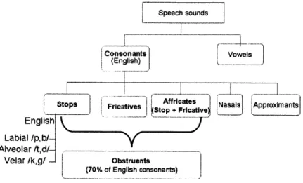
Fig. 1-1 Concept Map -Speech sounds are composed of vowels and consonants. English

consonants can be sub-categorized into stops, fricatives, affricates, nasals, and approximants, according the manner of articulation. Among them, stops, fricatives and affricates are also called obstruents, and this name implies obstruction of air in their production. In English, 70 percent of consonants are obstruents... ... 18

Fig. 1-2 (a) Midsagittal section of the vocal tract when a stop consonant /t/ is produced 11. The tongue blade is making a complete closure at the alveolar ridge. (b) Midsagittal section of the vocal tract when a fricative /s/ is produced [1I. The tongue blade is making a constriction at the alveolar ridge. (c) Acoustic waveform of the utterance /ata/. The closure interval, the interval of the /t/ sound, and the impulse-like transient are labeled. (d) Acoustic waveform of the utterance /asa/. The interval belonging to the /s/ sound is labeled... ... ... 20 Fig. 1-3 (a) The plateau-shaped release trajectory under the influence of the intraoral pressure (solid line) and the straight release trajectory without the influence of the intraoral pressure (dashed line). The labels with arrow indicate the time corresponding to the release sequences showed in the panels in (b)[11) .329. (b) Hypothesized sequences before and after the release of a

velar closure under the influence of the intraoral pressure (solid line) and without the influence of the intraoral pressure (dashed line). Owing to the intraoral pressure, the closure could be released before the time when the tongue dorsum leaves the palate without the influence of the intraoral

pressure [1] p329 .. ... 22

Fig. 1-4 (a) Midsagittal profile of the vocal tract when a supraglottal constriction is formed with the lips. Z9 and ZC are the impedance at the glottal and supraglottal constriction.11

(b) Equivalent circuit model for the air flow in the vocal tract configuration in (a): the voltage

source P, represents the subglottal pressure; Current source U, represents active expansion or contraction of the vocal tract volume; C, is the compliance of the air in the vocal tract volume; and R., M, and C, are the resistance, mass, and compliance of the vocal tract walls respectively.

[I]

... ... 2 5

Fig. 2-1 Concept map: the pressure-wall interaction models in relation to speech sounds... 29 Fig. 2-2 Left: Diagram of Stevens' 2-section model. (a) A typical tapered constriction with yielding wall. P,,, is the intraoral pressure and U is the volume velocity coming out of the constriction Pl. (b) The 2-section model used to represent the compliant constriction 1i. di and d2 are the height of the two sections respectively. Fig. 2-2 Right: The final height of the front section d2 calculated with the 2-section model versus its initial resting height d20 ['. d20 is the

height of the front section when P,, = P ... 31 Fig. 2-3 McGowan's sprung trap door model for the tongue-tip trill. P is the intraoral pressure

(10)

constriction formed with the tongue tip and the palate; U, is the volume velocity at the

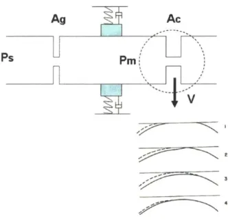
constriction; and LC is the thickness of the tongue tip. ... 35 Fig. 2-4 Concept map: vocal fold m odels... 36 Fig. 3-1 Lumped elements representing the soft tissue surface in the vicinity of the closure. The rigid target plane is represented by a straight dashed line above the lumped elements. The upper-mass represents the part of surface in contact with the target plane and the lower upper-mass represents the part of surface right behind the closure. (a) The configuration of the lumped elements during the closure interval. The force received on the lower mass is the intraoral pressure Pm and the force received on the upper mass is the contact pressure. (b) The configuration of the lumped elements when the closure is released. The force on the lower mass is the intraoral pressure Pm and the force on the upper m ass is P, . ... 42 Fig. 3-2 Simplified configuration of the vocal tract for demonstrating the pressure-flow along the vocal tract. P, is the subglottal pressure, Ag is the cross-sectional area of the glottal constriction,

Pm is the intraoral pressure, and Ae is the time-varying cross-sectional area of the supraglottal constriction at which the pressure-wall interaction occurs. The lower boundary of the supraglottal

constriction moves downward with a constant velocity V. The release events [II pp329 hypothesized

by Stevens are also attached for illustrating the big picture along the whole vocal tract... 46 Fig. 3-3 Two types of unsteady flow motion at the release of a complete closure: (a) the flow caused by the change in the cross-sectional area; and (b) the flow induced by the pressure

gradient along the released closure... 49 Fig. 3-4 Illustration of a system property transporting within a deformable control volume and the modified Reynolds Transport Theorem. The blue color marks the system occupying the control volume at time t; the orange color marks the extra substance flowing into the control volume from the environment during the time interval At . ... 50 Fig. 3-5 A control volume (in dashed line) used for deriving the governing equations in the unsteady incompressible flow model in a uniform tube with length LC and time-varying cross-sectional area A, (t) (not shown in the figure). The flow velocity at the inlet and the exit of the tube are u, and u, respectively, and the static pressure at the inlet is P , and P, at the exit. The

L

control volume shown in the diagram occupies a part of the tube with length LC - x. The left

2

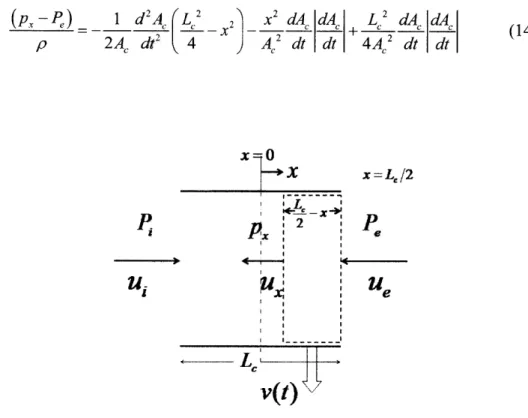
boundary of the control volume is at the location x, whose origin is in the middle of the tube, and the right boundary of the control volume is at the exit of the tube... 52 Fig. 3-6 A control volume (in dashed line) defined in a uniform tube with length L and time-varying cross-sectional area. The control volume has length x, with the left boundary at the location x and the right boundary at the exit of the tube. The flow velocity at the inlet and the exit of the tube are u, and u, respectively; the static pressure at the inlet is P; and the static pressure

at the exit is P,. The static pressure and the flow velocity at the location x are p, and u,

(11)

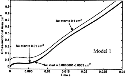
Fig. 4-1 The release trajectories of A, ,,,=0.0000001 cm2 to 0.1 cm2 _{calculated with Model 1}

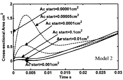
(quasi-steady incompressible flow). The release trajectories change little when A, 0.01cm2.. 62 Fig. 4-2 The release trajectories of A star, =0.00001 cm2 to 0.1 cm2 calculated with Model 2

(unsteady incompressible flow). The plateau becomes a peak when

0.00001cm2 _<_A,, _{< 0.001cm}2_{, and a straight line when A, ,,a,, > 0.00001cm2}_... . .. . . ₆₃

Fig. 4-3 The release trajectories of A, ,t,, =0.0000001 cm2 _{to 0.1 cm}2 _{calculated with Model 3}

(unsteady compressible flow). The magnitude of the plateau decreases with decreasing

A,,lrt until a zero cross-sectional area is reached at around 2 millisecond

w hen A, a,,,, = 0.00005cm 2 .. ... .... . .. . .. .. . .. . .. .. . . .. .. . .. . .. . .. .. . .. . .. . . . 64

Fig. 4-4 The release trajectories of length 4 = lcm and A, ', =0.001 cm2 calculated with the

three m odels ... ... 65 Fig. 4-5 The release trajectories of a closure with length 4 =0.1,0.5 and lcm and

A, ,,rt = 0.001cm 2 _{calculated with Model 1 (quasi-steady incompressible flow).} _{... 66}

Fig. 4-6 The release trajectories of a closure with length L, = 0.1,0.5 and lcm and

Ac start = 0.001cm2 calculated with Model 2 (unsteady incompressible flow)... 67

Fig. 4-7 The release trajectories of a closure with length L, = 0.1,0.5 and lcm and

A _start = 0.00 lcm2 calculated with Model 3 (unsteady compressible flow)... 67

Fig. 4-8 The release trajectories of a closure with L, = l and 0.5cm and A. = 0.00005cm2 ,

calculated with Model 2 (unsteady incompressible flow)... 68 Fig. 4-9 The release trajectories of a closure L, = 1,0.5, and 0. lcm and A = 0.0001cm2

calculated with Model 3 (unsteady compressible flow)... 69 Fig. 4-10 The /p/-release trajectories calculated with Model I (quasi-steady incompressible flow)

... ... 7 1 Fig. 4-11 The /t/-release trajectories calculated with Model 1 (quasi-steady incompressible flow)

... ... 7 1 Fig. 4-12 The /k/-release trajectories calculated with Model I (quasi-steady incompressible).... 72 Fig. 4-13 The /p/-release trajectories calculated with Model 3 (unsteady compressible)... 73 Fig. 4-14 The /t/-release trajectories calculated with Model 3 (unsteady compressible)... 73 Fig. 4-15 The /k/-release trajectories calculated with Model 3 (unsteady compressible)... 74 Fig. 5-1 The waveform of a /t/-release (in blue line) from the sentence "Don't ask me to carry an oily rag like that." (TIMIT\train\dr2\faem0\sa2). The average FFT magnitude Av in the whole frequency range (in black line), and the magnitude Ap in a frequency band containing the front cavity resonance (in red line). The duration of the frication noise is indicated as 23 ms. It is the duration between the start of the release and the time when Ap (in red line) starts to drop rapidly,

(12)

at the same time, Ap is at least twice of Av, then corrected by adding the window length of 5

m illiseconds... ... 8 1 Fig. 5-2 The waveform of a /k/-release (in blue line) from the sentence "Don't ask me to carry an oily rag like that." (TIMIT\train\dr2\fcaj0\sa2). The duration of the frication noise is 45 ms... 81 Fig. 5-3 The waveform of a /k/-release (in blue line) from the sentence "Don't ask me to carry an oily rag like that." (TIMIT\train\dr2\ faem0\sa2). The duration of the frication noise is 38 ms... 82 Fig. 5-4 An examples of a /k/ release with dominant frication noise throughout the release burst.

... 8 3 Fig. 5-5 (a) Waveform and spectrogram of utterance /uhtA/; (b) Waveform and spectrogram of utterance /uhdA/. Formants are tracked automatically with a code written by Mark Tiede, and are shown in the spectrogram in blue, green and read thick lines. The onset of release starts around 400 ms in both /t/ and /d/. In (a), the formants are straight without any apparent movements after the voicing onset following /t/; while formant movements can be observed right after the release o f /d/. ... 8 5 Fig. 5-6. A portion of the tongue making a complete closure of length Lc. The soft tissue surface of the tongue is represented as a layer of springs with stiffness k per unit area. Part of the tongue surface is in contact with the palate and part of it is exposed to the intraoral pressure P. The intraoral pressure compresses the tongue surface downward of height h and also applies a horizontal force of fp on the part of the tongue in contact with the palate. This force is balanced by the frictional force

f,

between the surfaces in contact. Shear forces inside the tissue of the articulator are neglected. ... ₈₈ Fig. B- 1 (a) Pressure Pm inside a circular tank with radius R and thickness d. Tension ot inside the wall. (b) The tissue wall during the closure interval of a bilabial stop consonant /p/ can be taken as part of the wall of a tank against intraoral pressure Pm. 107

(13)

List of tables

T able 3-1 E quation set... .1... 60

Table 4-1 Duration of the plateau of voiceless stop consonants calculated with Flow model 1 (quasi-steady incompressible) and 3 (unsteady compressible)... ... 74 Table 5-1 Comparison of the durations measured in the acoustic signal, calculated with two flow

m odels m odels, and estim ated by Stevens 48]... ... ... 84

(14)

(15)

List of symbols

A, Cross-sectional area of the supraglottal constriction

Ac-start Cross-sectional area of the supraglottal constriction at the time of release

A9 Cross-sectional area of the glottal constriction

CV Control volume

D Length of the supraglottal constriction along the dimension

perpendicular to the midsagittal plane

d Derivative

Fp Average pressure force acting on the upper mass

FL F, Force generated by the spring connecting the two masses

fp. Horizontal pressure force

fk Kinetic frictional force

f, Static fictional force between the contacting surfaces

he Downward displacement of the tongue surface

k Lumped spring constant or the stiffiess of the soft tissue surface

ke Spring constant connecting the two masses

L Inductance

L, Axial length of the supraglottal constriction

m Lumped mass of the soft tissue surface

Prel Contact pressure at the time of release

Static pressure at the exit of the tube Static pressure at the inlet of the tube

P Intraoral pressure

Subglottal pressure

P, Static pressure at the location x

r Lumped damping of the soft tissue surface

t Time

U Volume velocity going through the supraglottal constriction

Ug Volume velocity going through the glottis

Ux Flow velocity at the location x

V Constant release velocity

V Instantaneous downward velocity of the upper mass

Y1 Displacement of the upper mass

Yeq 1 Equilibrium position of the upper mass

(16)

Yeq2 Equilibrium position of the lower mass

p Density of the air

pI Maximum static frictional coefficient

(17)

Chapter 1 Introduction

1.1 Research background

Speech is the most convenient way of human communication. A person may not realize any difficulty in speaking his/her own native language, but when he/she starts to

learn a foreign language, production problem occurs. Some patients with diseases such as Parkinson's and ALS (Amyotrophic lateral sclerosis), take even greater effort in

producing an understandable speech sound. He/she needs to know how and be able to produce the correct sound so that others can understand the word being expressed.

Speech is also the most convenient means of man-machine communication. In this task, a computer is expected to recognize human speech accurately, which is called automatic speech recognition; and also to "speak" as naturally as a human speaker, which is realized by speech synthesis.

Human speech is powered by the pulmonary pressure in the lung. The air coming out of the lung interacts with various structures along the vocal tract (the air way from the throat to the lips), and generates the sound sources, which are then filtered by the cavity resonances determined by the shape of the vocal tract when the particular speech sound is produced. Both generating the sound sources and shaping the vocal tract require the coordination of multiple respiratory and articulatory structures.

As a special type of sound, speech is the subject studied in speech production, a discipline under acoustics. Acoustics studies the generation, propagation, and reception of sound. Similarly, speech production studies speech sound generation and propagation along the vocal tract of a human subject. The perception of speech sound is studied in speech perception, or psychoacoustics. Based on the physics of speech sound generation and propagation, mathematical models are developed as tools for quantifying the physiological activities involved in producing a speech sound.

(18)

Speech production models also provide a knowledge-based approach to identify features of the speech sound for speech recognition [21, and supply rules for speech

[31 synthesis

Speech sounds are composed of two primary categories: vowels and consonants. In the production of a vowel, vocal fold vibration is present and the sound source is located at the laryngx. In producing a consonant, the vocal folds do not vibrate, or vibrate in a more moderate mode compared with the vibration in producing a vowel.

Speech sounds

Consonants Vowels

(English) 9

Stops Fr catives tpFcate Nasal Approximants

kStop. +Fricatve S English Labial /p,b/ Alveolar /t,d/-Velar /k,g/ Obstruents (70% of English consonants)

Fig. 1-1 Concept Map - Speech sounds are composed of vowels and consonants. English consonants can be sub-categorized into stops, fricatives, affricates, nasals, and approximants, according the manner of articulation. Among them, stops, fricatives and affricates are also called obstruents, and this name implies obstruction of air in their production. In English, 70 percent of consonants are obstruents.

Effective use of the vowel models started from Chiba and Kajiyama [41 in 1941 for

the Japanese language, and the vowel models for the English language were first reported by Jakobson, Fant, and Halle [51 in 1952. Later, Fant's work in 1960 [6], "Acoustic Theory

of Speech Production", established the theoretical framework widely and currently used. Compared to the vowel models, slow advance has been made in the consonant models [7] pp2930. One of the obstacles, considered by Fant, is the difficulty involved in

(19)

According to the way of producing the sound (also called manner of articulation by phoneticians), English consonants can be further grouped into stop consonants, fricatives, affricates, nasals, and approximants, as shown in the concept map in Fig. 1-1. Among them, stop consonants, fricatives, and affricates are also called obstruent

consonants. The name "obstruent" means that obstruction of air exists in their production. In English, 70 percent of consonants belong to obstruent consonants.

In this group with the largest number of consonants, stop consonants (/p, b, t, d, k, g/) and fricatives (/f, v, s, z,

f,

3, 0, 6/) comprise the majority, and the remnant of two affricates (/f, d3/) can be taken as the combination of a stop consonant and a fricative.

The articulation and the acoustics of a stop consonant /t/ and a fricative /s/ are compared in Fig. 1-2. The midsagittal profile of the vocal tract in producing the closure interval of /t/ is shown in Fig. 1-2a, and the profile in producing /s/ is shown in Fig. 1-2b. A complete closure is made with the tongue tip for /t/ and a constriction is made for /s/, both at the alveolar ridge. Air pressure is being built up behind either the closure or the

constriction.

The acoustic waveform of utterance /ata/ and /asa/ are shown in Fig. 1-2c and Fig. 1-2d respectively. The closure interval in the acoustic waveform of /t/ is indicated in Fig. 1-2c, corresponding to the articulation profile shown in Fig. 1-2a. No sound is supposed to be produced during this interval, and the signal recorded in the acoustic waveform belongs to the background noise. When the closure is released, a brief interval of turbulence noise is generated immediately from the air stream coming out from the released closure. This interval is labeled as "/t/" in the acoustic waveform in Fig. 1-2c. In producing the fricative /s/, an air stream goes through the constriction shown in Fig. 1-2b, and creates continuous turbulence noise. This interval is indicated by the label "/s/" in the acoustic waveform in Fig. 1-2d. Both acoustic waveforms demonstrate that turbulence noise is characteristic of obstruent consonants. A stop consonant distinguishes itself from a fricative at the onset of the turbulence noise, where an initial transient is generated first. The transient looks like an impulse in the waveform (Fig. 1-2c) at the beginning of the /t/ interval.

(20)

b

5

D (tl) ( c) ,~~~~ ,Q4t) .~: * a a3 M 3 to TUWrs1 ( d)

Fig. 1-2 (a) Midsagittal section of the vocal tract when a stop consonant /t/ is produced [ll. The tongue blade is making a complete closure at the alveolar ridge. (b) Midsagittal section of the vocal tract when a fricative /s/ is produced [1. The tongue blade is making a constriction at the alveolar ridge. (c) Acoustic waveform of the utterance /ata/. The closure interval, the interval of the /t/ sound, and the impulse-like transient are labeled. (d) Acoustic waveform of the utterance

/asa/. The interval belonging to the /s/ sound is labeled.

As the name "obstruent" suggests, obstruent consonants are produced with obstruction of air in the vocal tract. In the course of obstructing the air, a soft tissue articulator (it is often the primary articulator utilized in producing the consonant) such as the tongue blade, the tongue dorsum, or the lower lip, is always involved to make a

WI-7L

1 1 1 1 1 I &t j J l l

(21)

complete closure with the target surface in producing a stop consonant, or to create a constriction in the airway in producing a fricative. Air pressure is then built up in the vocal tract, and this increase in air pressure is necessary for generating the turbulence noise characteristic of these consonants.

Stevens discussed the role of the yielding surface of soft-tissue articulators in the articulatory models of stop and fricative consonants [1] pp 325, 328-329, 382 respectively. He created a model of the interaction of steady flow with the yielding wall in fricative production, which showed that the compliant surface makes it easier for the speaker to

generate the turbulence noise with the maximum intensity at the supraglottal

constriction[' 1 10-111. He also considered the pressure-wall interaction during the release of a stop closure, and his hypothesis serves as the motivation of this thesis, as discussed in the next section.

1.2 Motivation: Stevens' hypothesis

Stevens [II pp 329-330 suggested that the pressure-wall interaction would lead to a

plateau-shaped release trajectory shown in solid line in Fig. 1-3a. He also illustrated schematically in the panels in Fig. 1-3b the hypothesized sequences of events after a velar closure is released.

The mechanism underlying his hypothesis was that the pressurized air behind the closure may cause the closure to be released (in solid line) earlier than the time when it would be without the influence of the intraoral pressure buildup (in dashed line). After the release, owing to the decrease in intraoral pressure, the compliant tissue surface would bounce back, and a plateau in the release trajectory could be retained for a while when the tongue dorsum keeps moving downward. The slower this downward motion, the longer the plateau could be retained.

Hanson and Stevens 18] found perceptual evidence for this hypothesis: the stop consonants were perceptually more "acceptable" when they were synthesized with a plateau progressively longer for labial, alveolar, and velar in the release trajectories, and they had acoustic characteristics matching better to normal speech.

(22)

palate IN -2 -doru0 05 2of E /Q% tongue 414

TIME (

ms)

(a)

(b)

Fig.1-3 (a) The plateau-shaped release trajectory under the influence of the intraoral pressure

(solid line) and the straight release trajectory without the influence of the intraoral pressure (dashed line). The labels with arrow indicate the time corresponding to the release sequences showed in the panels in (b)[11 pp329. (b) Hypothesized sequences before and after the release of a

velar closure under the influence of the intraoral pressure (solid line) and without the influence of the intraoral pressure (dashed line). Owing to the intraoral pressure, the closure could be

released before the time when the tongue dorsum leaves the palate without the influence of the

intraoral pressure [1] pp329

However, it is difficult to measure this plateau-shaped release trajectory directly because (1) the pressure-wall interaction may last for very short time, on the order of tens of milliseconds; (2) the dynamic range of the displacement of the yielding wall is so small that a good space resolution at the tissue boundary is required; (3) the systems capable of tracking articulatory movements with X-ray or EM-waves can not capture the release trajectories right at the closure, as the sensors are intentionally placed away from

[9]

the location of the closure, in order to prevent interference with speech production This situation fits what Fant [7] pp29-30 commented about the slow advance in

consonant models compared with vowel models. He considered that "the obstacles are our lack of reliable data on the details of the vocal tract and reliable physiological data

(23)

with respect to consonants, and also the difficulty involved in modeling all relevant factors in the acoustic production process".

1.3 Objective and thesis outline

We initially aim to test Stevens' hypothesis by developing a mathematical model of the pressure-wall interaction during the release of a stop closure. This effort would contribute to a more complete scientific pursuit of the physiology of consonant production.

Relevant knowledge in speech production is introduced in the next section, which includes speech aerodynamics, mechanical properties of the compliant tissue walls, turbulence noise source in speech production, the place of articulation, and the acoustics of stop consonants.

Previous studies on the pressure-wall interaction in speech production are reviewed in Chapter 2. Stevens' fricative model mentioned in Section 1.1 is introduced

first, which studied the type of consonants closest to stop consonants. Another consonant model, McGowan's tongue tip trill model, is introduced next, which studied the

interaction of an unsteady flow the yielding wall. At last, vocal fold models are introduced.

New models developed in this thesis for the pressure-wall interaction in stop consonant production are discussed in Chapter 3. The results calculated with these models are presented in Chapter 1. Comparison of the model results and relevant acoustic data are discussed in Chapter 5, and also an unknown parameter in the models is

(24)

1.4 Relevant knowledge in speech production: speech aerodynamics,

compliant walls, turbulence noise source, the place of articulation, and

the acoustic pattern of stop consonants

In this section, some concepts and knowledge in speech production theory are introduced. They are referred to in the following chapters.

1.4.1 Speech aerodynamics and compliant walls

Speech aerodynamics studies the pressure and flow along the vocal tract, the air way between the throat and the lips, which can be simplified as a tube with cross-sectional area variable both in time and along its axis (Fig. 1-4a). The configuration of the vocal tract is determined by the positioning of the articulators such as the tongue, the lips, and the jaw, which move continuously during speech production.

As the most active articulator, the tongue functions not only to modify the shape of the vocal tract, or the acoustic characteristics in the radiated sound, but also works as a valve for either inhibiting or stopping the flow of air in the mouth. Working together with the teeth, alveolar processes, and the palate, the tongue is a part of the noise generator in the vocal tract. [10]

The pressure and flow in the vocal tract has been studied with a circuit model shown in Fig. 1-4b. 111 _{Pressure P is represented as potential and volume velocity U is}

represented as current. Lumped elements in the circuit model represent aerodynamic properties along the vocal tract and relevant physiological activities such as forming a supraglottal constriction or full closure, adducting or abducting the glottis, adjusting the stiffness of the vocal tract walls, and active expanding or contracting the vocal tract.

Below the glottis (the space between the vocal folds which is shown as an elliptic circle located at the inferior end of the vocal tract in Fig. 1-4a), a constant pressure P, is assumed during speech production. This pressure is represented as a voltage source with magnitude P, in the circuit model shown in Fig. 1-4b. Z, is the resistance of the

(25)

For constrictions with the dimensions encountered in speech production, an 1 U

empirical pressure-flow relation AP = p( )2 [1 pp can be applied. This relation comes 2 A

from an average of the coefficient kL (in AP = k -p( )2) measured by Heinz 12 and Jw.

2 A

van den Berg et al. 13] Subsequently, resistance Z, and Zg are obtained from

APl1

Z- A=- pU at the particular location, and they are nonlinear elements in the circuit.

U 2

The movement of the jaw and some laryngeal structures can actively expand or contract the volume of the vocal tract. This volume change is represented as a current source Ua in the circuit.

z

Z

wR

C --S Z(b)

C

w P_S (a)

Fig. 1-4 (a) Midsagittal profile of the vocal tract when a supraglottal constriction is formed with the lips. Z9 and ZC are the impedance at the glottal and supraglottal constriction.11

(b) Equivalent circuit model for the air flow in the vocal tract configuration in (a): the voltage

source P, represents the subglottal pressure; Current source U, represents active expansion or

contraction of the vocal tract volume; C, is the compliance of the air in the vocal tract volume; and RW , M, and C,, are the resistance, mass, and compliance of the vocal tract walls

(26)

A significant deviation from common duct flow is caused by the massive yielding walls of soft tissue surfaces along the vocal tract, with only a small portion of hard wall along the teeth and the hard palate. The yielding walls can be put into motion by pressure variations in the vocal tract, and the degree of mobility is described by the inverse of their mechanical impedance per unit area [I pp26, which is defined as the ratio of the pressure acting on the wall over the resulting velocity. The impedance in the frequency range up to 100 to 200 Hz is the combination of a compliance C,, a mass M, , and a resistance

1

R,in series, Z, = _{+ 0jM, +R, .}

ja>C, i

Based on the impedance measured on cheek tissue conducted by Ishizaka, et al. [141 , _{the ranges of the three elements (in per unit area) were estimated as}

C, ~.0x10-5to3.Ox i- 5 cm3 _dYne

M, ~ 1.0 to 2.0 gm/cm2 R, - 800 to 2000 dyne - s/cm'

Svirsky et al. [15] also measured the in-vivo compliance C, of the tongue surface by tracking the displacement of a flesh point during the closure portion of voiced and voiceless stop consonants. The recorded displacements were averaged to derive the

surface compliance, which showed the same order as the impedance estimated by

Ishizaka et al. [14] Additionally, they found that the surface compliance was about 3 times

larger for a voiced than for a voiceless stop consonant. The more compliant tongue surface in producing a voiced stop consonant had been considered as a means of maintaining voicing at the glottis .16]. In a pressurized tank model of making a stop closure later discussed in Appendix B, the difference in stiffness also results from the force balance required under difference levels of intraoral pressure buildup.

The impedance in per unit area introduced above is used to derive the elements Cw, Mw , and R, in the circuit model shown in Fig. 1-4b. For a surface area S of the

(27)

walls between the glottis and the supraglottal constriction, multiplying C, by the area S

gives C,, and dividing M, and R, by the area S respectively gives M, and R, .

The last element C, in Fig. 1-4b represents the volume compliance of the air in

the vocal tract. As a small quantity compared with the wall impedance, this element is often neglected.

1.4.2 Turbulence noise source and the place of articulation

The acoustic signal of obstruent consonants is characterized by the dominance of wideband noise, which is generated by the jet coming out from a narrowing called constriction in the vocal tract. This type of sound source is also called turbulence noise source because it is generated by the turbulence in the jet.

The turbulence noise source in obstruent production is located near to a

constriction in the vocal tract. Once the pressure and flow along the vocal tract have been derived with the circuit model introduced above, the intensity of the turbulence noise sources can be estimated from empirical equations. Experiments with mechanical modelsr1 7₁_{found that the sound power in the middle- and high- frequency range of the} turbulence noise source generated at the constriction is proportional to the third power of the pressure buildup behind a constriction. For a given cross-sectional area A and a pressure drop APm across the constriction, the magnitude of the turbulence noise source is

3!1

derived as: p, = KAP,,IA 2 _{(K is a constant determined by the flow rate and the specific} configuration of the constriction).

The turbulence noise source at the constriction is then filtered by the front cavity, which is the space between the constriction and the lips, and the spectrum of the radiated sound usually has a prominence at the frequency corresponding to the lowest natural frequency of the front cavity, also called the front-cavity resonance. As this resonant frequency is inversely proportional to the length of the front cavity, it gives information about the location of the constriction.

(28)

The location of the constriction is also called the place of articulation by

phoneticians, as it is the'place where an articulatory closure or constriction is made. The frequency of the front-cavity resonance has been found an important cue for identifying the place of articulation of obstruent consonants [183-20], [i]

1.4.3 The acoustic pattern of stop consonants

The acoustic events following the release of a stop consonant have been described by Fant [61. The sequence starts with a brief pulse of volume velocity, which is called the initial transient. The transient is then followed by a burst of turbulence noise source called the frication noise, which locates at the constriction; and then a possible brief interval of turbulence noise source called the aspiration noise, which is generated at the glottis.

During the first 1-2 ms of the release, the air flow is accelerated by the pressure gradient across the released closure. This transient flow generates a sharp impulse at the released closure. The impulse contains the most accurate information of the place of articulation without any smearing from noise, and it could be a perceptually important cue to the place of articulation. However, with weak energy, this impulse was often found buried in the frication noise. [22]

Following the transient, the frication noise is generated by the air stream coming out of the released closure. The frication noise also contains the front-cavity resonance, thus providing information about the place of articulation.

Following the frication noise, the aspiration noise may be generated by the air stream at the glottal constriction, when the glottis is adducted for voicing. The aspiration noise does not contain salient information of the front cavity; because it is located at the glottis.

In English, a stop consonant may be produced at three different places of articulation: bilabial (at the lips, /p/ and /b/), alveolar (with the tongue tip and at the alveolar ridge, /t/ and /d/), and velar (with the tongue body and at the soft palate, /k/ and /g/).

(29)

Chapter 2 Literature review: previous studies on the pressure-wall

interaction in speech production

At present, only two models have been found in the literature addressing the pressure-wall interaction in consonant production: McGowan's sprung-trap-door

model23₁_{for tongue-tip trills and Stevens' 2-section modeli Ipp 109-112}_{for the influence of} steady flow on the yielding wall in the vicinity of a constriction in fricative production. In contrast, a large number of mathematical models have been developed for the vibration of vocal folds in the presence of air stream. [24][301

The relation of these models to speech sounds is indicated in the concept map in Fig. 2-1. The model developed in this thesis is also included.

Fig. 2-1 Concept map: the pressure-wall interaction models in relation to speech sounds.

As Steven's model addresses fricatives, which is the type of consonants closest to the subject of this thesis, stop consonants, his model is discussed in more details.

McGowan's tongue tip trill model focused on the role of the compliance of the vocal tract wall in sustaining the tongue-tip vibration. English does not have trill sounds. They are

.

(30)

special consonants in some languages such as Italian and Russian, and they can be categorized as approximants.

Both consonant models did not treat the collision of the primary articulator with the target plane, because collision is negligible in their cases; however, in stop consonant production, the motion of the primary articulator starts from a collided condition - the primary articulator in contact with the target plane, so the collision cannot be neglected.

The collision leads to a contact force between the primary articulator and the target plane, and in Section 5.3 a proper amount of contact pressure is demonstrated to be a necessary condition to retain a complete seal when air pressure is built up. The

importance of the contact force in making a complete closure was also suggested by L6fqvist A. et al. [31] The contact force needs to be treated in a more complete stop

production model.

In contrast to the small number of consonant models addressing the pressure-wall interaction, a larger number of models have been developed for the pressure-wall

interaction in vocal fold vibration, and some of them have also treated the collision. The vocal fold models are not going to be covered in details because of the large amount. As the new model developed for stop consonants in this thesis is similar to the famous two-mass vocal fold model251 in many aspects, more details about this vocal fold model is introduced in the next chapter.

As regards the type of flow in these models, Stevens' 2-sectional model deals with steady flow; while in both McGowan's model and the two-mass vocal fold model, the flow is unsteady, which is also characteristic of the flow in the release of a stop closure.

(31)

2.1 Steven's 2-section model for fricative production

Stevens [I] 0 used a 2-section model ( Fig. 2-2 Left (b) ) to represent the yielding wall in the vicinity of a constriction in fricative consonant production. The tube with two sections of height di and d2 respectively, represents a typical tapered

constriction with yielding wall shown in Fig. 2-2 Left (a), The section with height d2 corresponds to the region with the minimum cross-sectional area.

V OA-z (a) pU IL 0

d,~__jd2

0.10 b0 (b) _d-0 CM When0- _0,.P _-0.1" 0 _. ₀I_.2 a3s a

hen.= P,,andnoairflowgoes RESTING WIDTH OF FRONT SECTION d20 (cm) through the constriction, d,= d2,.

Fig. 2-2 Left: Diagram of Stevens' 2-section model. (a) A typical tapered constriction with yielding

wall. P,, is the intraoral pressure and U is the volume velocity coming out of the constriction 1]. (b)

The 2-section model used to represent the compliant constriction . di and d2 are the height of

the two sections respectively. Fig. 2-2 Right: The final height of the front section d2calculated with the 2-section model versus its initial resting height d,, 1. d2, is the height of the front

section when P P, .

For such a compliant tube, the initial height of the front section is d20 without air

flow, and the height becomes d2 when a steady air flow goes through the tube after the

(32)

with height d2 determines the intensity of the turbulence noise, and it is also referred to as

the size of the constriction.

The 2-section model has two parameters: the surface compliance per unit area C, and the difference Ad between the height of the front section (d2 ) and that of the

adjacent upstream section (d,), indicating the degree of tapering. They are assumed to be constant in producing a fricative.

The model calculated the final height d2 versus the initial height d20 , and the

result is plotted in Fig. 2-2 Right for different degrees of tapering Ad. This result showed that the presence of the air flow enlarged the size of the fricative constriction and the amount of increase depends on the degree of tapering Ad, and the initial size of the constriction.

The model results also suggested that a yielding wall also makes it easier to form a supraglottal constriction whose cross-sectional area is optimal for generating turbulence noise with the maximum intensity at the constriction. Based on the pressure-flow relation and the empirical equation of the intensity of turbulence noise source introduced in the previous chapter, it has been found that when the cross-sectional area of the supraglottal

constriction is i/N5d times the glottal constriction area, the maximum turbulence noise intensity can be achieved at the supraglottal constriction"1 P410-111, for a constant subglottal pressure and fixed glottal constriction area.

As the glottal constriction area is estimated to be in the range of 0.1 ~ 0.3 cm2 when a male speaker produces a voiceless fricative11 _{NP4-11, the optimal}

supraglottal constriction area for the voiceless fricative is in the range of 0.04-0.13 cm2_. For a constriction width of 2 cm, the height is 0.02-0.065 cm in the vertical dimension. To achieve this small range of constriction area, precise control over the positioning of the primary articulator is required. However, from Fig. 2-2 Right, we know that this range of d₂corresponds to a wider range of d20 up to 0.1 cm because of the pressure-wall

(33)

interaction, thus it becomes easier for the speaker to adjust the constriction size to be within the optimal range ".

Additionally, the optimal range includes negative initial heights. A negative initial constriction area means that a complete closure is initially made because of a

displacement intruding the roof of the constriction. The resultant contact pressure and the rich distribution of sensory receptors along the palate and the tongue could also

contribute to the ease of control over both the vertical and axial positioning of the primary articulator.

Stevens' model suggested that an initial complete closure is allowed in producing a fricative; however, it also has a limitation which suggests that a negative initial height can always go above zero as long as there is any tapering in the shape of the constriction (Fig. 2-2b), and it is impossible to make a complete closure against air pressure buildup. As we know from the production of a stop consonant, when the initial height of a constriction is negative enough, the intraoral pressure will not be able to open it, and a complete closure can be retained before it is released.

(34)

2.2 McGowan's sprung trap door model for the tongue tip trills

Trill is a special type of speech sound presented only in some languages such as Italian and Russian. They are produced by sustained vibration of a soft tissue articulator. The model introduced here addressed the trill sounds produced with the tongue tip, but other articulators such as the lips and other parts of the tongue can produce trill sounds too.

McGowan [23] created a model of the tongue tip interacting with unsteady air flow

in a sustained vibration, and quasi-steady flow was assumed (Fig. 2-3). The tongue-tip articulator was treated as a sprung trap door, moving under the combined action of the Bernoulli force in the air flow and the intraoral pressure P behind the "door".

The tongue tip model has a moment of inertiaI, and it is hinged on the rest part of the tongue by springs, with a rest angle 0 relative to the vertical direction. In deriving the moment of inertiaI , the tongue tip is modeled as a rectangular beam with height hT , thickness le and breadth (dimension into the paper) bT. The parameter AC represents the

cross-sectional area of the constriction between the tip of the tongue and the palate, and UC is the volume velocity coming out of this constriction.

The constriction area AC and the intraoral pressure Pc are related in a nonlinear differential equation governing the motion of the "door":

d2_{9 rd9}

K V

-+ -- + -(1+ 102)0 =

dt2 _I_dt _I _I

In this equation, 0 is the rest angle; I = PTcbr (hT /3); AC = bThT[i - cos(0)]; K and

7/K are linear and cubic spring constants; r is the resistive constant in the tongue tip; and pT is the density of the tongue tip. r is the torque exerted by the air pressure, derived

2

as1r = bThT2 P - K is the density of the air, and K is a parameter that

(35)

quantifies the reduction in static pressure surrounding the tongue-tip surface because of the Bernoulli effect.

Pc

Axis of rotation

Fig. 2-3 McGowan's sprung trap door model for the tongue-tip trill. P is the intraoral pressure upstream of the constriction; 0 is the rest angle; A, represents the cross-sectional area of the constriction formed with the tongue tip and the palate; U, is the volume velocity at the

constriction; and L. is the thickness of the tongue tip.

The intraoral pressure P is then related to the compliance and other lumped

mechanical properties of the vocal tract wall behind the tongue tip by means of electrical circuit analogy. In order to solve these governing equations, McGowan had to estimate the order of magnitude of quite a few parameters with and without the aid of

(36)

2.3 Vocal fold models

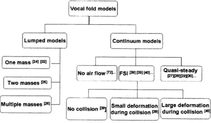
Small deformation Large deformation during collision P9] during collision [4

Fig. 2-4 Concept map: vocal fold models

The vocal folds have been simulated with lumped-element models, such as the one-mass modelt241_,[32_],_two-mass_modelt251 _{and multi- mass models[}26_],_{and also the}

continuum models[27_{j,[28],[29j,30,[72]}_{(Fig. 2-4).}

Most vocal fold models treat the pressure-wall interaction under the quasi-steady assumption, which validates the application of the flow variables obtained on a static vocal fold model to the vocal folds in motion [331, [341, _{except for a short time before the}

vocal folds are collided and after they are separated apart.[351,[361,[371

Some models [381,[391,[401 _{do not require the quasi-steady assumption to apply the}

empirical relations. They calculate the deformation of the vocal folds and the air flow between them simultaneously before coupling the solutions in both domains together. This process is also called FSI (Fluid-structure Interaction). Among these FSI vocal-fold models, Tao and Jiang [381 did not treat the collision; Luo et al.[39] treated small

deformations caused by the collision; and an FSI continuum model capable of treating large deformations during the collision has recently been developed by Zhang et al. [40.

The famous two-mass model developed by Ishizaka and Flanagan [25] is a widely

used lumped-element model. It can deal with the collision regardless of the degree of resultant deformation; however, it requires the quasi-steady assumption.

(37)

With similar method applied to the two-mass model, we first formulate a model devoted for the release of a stop closure in the next chapter. The stop consonant model differs in that the two masses representing the yielding surface of the primary articulator have an additional uniform rigid body motion. In vocal folds vibration, the rigid body motion of the folds is negligible. Moreover, at the time of release, an initial deformation due to the contact pressure at the time of release exists in the stop model.

Like the two mass model, quasi-steady flow is assumed in the first stop consonant model. The model is then further improved by relaxing the quasi-steady flow assumption, and two unsteady flow models are developed: unsteady incompressible and unsteady compressible flow.

(38)

(39)

Chapter 3 Analyses of the pressure-wall interaction during the

release of a closure

A stop consonant is produced by creating a complete closure in the air way with the primary articulator, and then air pressure is built up behind the closure. During the closure interval, a yielding wall in the vicinity of the closure is essential to prevent the air from escaping, functioning as an O-ring seal used in tubing systems containing fluids.

Furthermore, a proper amount of contact pressure is required between the two surfaces in contact for effective sealing. Both this contact pressure and the intraoral pressure buildup during the closure interval act on the yielding wall as external forces. Therefore, certain amount of elastic energy has already been stored in the wall before the release starts.

After the closure is released, the contact pressure disappears and the air pressure in the vicinity of the released closure drops suddenly, the yielding wall would move in respond to this change in the external forces. The resultant motion would again change the cross-sectional area of the released closure, and also the surrounding air pressure.

This interaction of the air pressure and the yielding wall is analyzed in this chapter. Since releasing the closure is accompanied by a rapid airflow which produces a burst of sound composed of a brief initial transient and turbulence noise, with duration of a few tens of milliseconds, the pressure-wall interaction would affect the airflow, and

eventually influence the generated sound.

In order to analyze the pressure-wall interaction, a solid model of the yielding wall and a flow model of the air flow going through the released closure are required, and then the two models are solved simultaneously.

(40)

The goal of the analysis is to calculate the evolution of the cross-sectional area Ac (t) after the closure is released, also called the release trajectory. Stevens

hypothesized a plateau-shaped release trajectory, as shown in Fig. 1-3a, so we first hope to find out if a plateau really exists in the calculated release trajectory. If a plateau does exist, we also hope to know how long it lasts during each type of release, as this duration would determine the duration of the frication noise in the acoustic signal of the particular type of stop consonant.

3.1 Solid model

A lumped-element solid model is developed to represent the viscoelastic

properties of the soft tissue surface of the primary articulator (the lower lip, the tongue tip, or the tongue body in English). Like the two-mass model of vocal folds, this solid model of the soft-tissue articulator is composed of two masses, three springs, and two dampers, as shown in Fig. 3-la. The upper mass represents the part of the surface in contact with a rigid target plane when a closure is formed, and the lower mass represents the part of the surface exposed to the intraoral pressure.

Two masses are applied to represent the soft tissue surface in the vicinity of the closure, as the part of the surface right at the closure and that upstream of the closure do not move in phase because the pressure forces acting on them are different. Consequently, different amount of potential energy is stored in them at the time of release.

The same per-unit-area value of the mass (m), spring constant (k), and damping coefficient (r) are assigned to the elements belonging to the two parts of surface, as the properties of the soft tissue surface can be assumed uniform in the vicinity of the closure. These quantities are determined according to the experiments done by Ishizaka et al. on the relaxed cheek tissue (refer to Appendix A for choosing the measured value of relaxed versus tense cheek tissue), The spring constant k, connecting the two masses is determined as 1.5k according to the convention used in the two-mass model of the vocal folds [25]

(41)

The target plane is assumed to be rigid and it is represented by a straight dashed line in the 2-D model shown in Fig. 3-1. This line represents the palate for alveolar and velar stop consonants (refer to Section 1.4.3, and Fig. 1-I); and for bilabial stop

consonants, it represents a virtual plane of symmetry between the two lips.

During the release, the base of the two-mass system moves downward with a constant velocity V, as shown in Fig. 3-1. The subsequent displacement of the upper mass y, (t), with t representing the time, would lead to a change of y, (t) D in the cross-sectional area of the supraglottal constriction (D is the length of the constriction along the

dimension perpendicular to the midsagittal plane.). The real-time cross-sectional area of the released closure is thus

(42)

Static pressure = Pm y2 = 0 (a) Static pressure = Pm Pm Static pressure = P1 Ac

(b) _{Downward movement with} constant velocity V

Fig. 3-1 Lumped elements representing the soft tissue surface in the vicinity of the closure. The rigid target plane is represented by a straight dashed line above the lumped elements. The upper-mass represents the part of surface in contact with the target plane and the lower upper-mass

represents the part of surface right behind the closure. (a) The configuration of the lumped elements during the closure interval, The force received on the lower mass is the intraoral pressure Pm and the force received on the upper mass is the contact pressure. (b) The

configuration of the lumped elements when the closure is released. The force on the lower mass is the intraoral pressure Pm and the force on the upper mass is P1.

y1 + y2 +

(43)

The governing equations of the motion of the two masses are formulated in they, - and they2 -coordinate respectively, as shown in Fig. 3-la. Both coordinates move

downward with a constant velocity V, so they are inertial coordinates. In each coordinates, the position of the mass at the time of release is set as the origin.

According to Newton's second law, the governing equation of the upper mass m, is formulated as:

m d2 _{dy, +}_{k y}

1 - y = Fk + F (2)

dt ' dt

Fk, =-ky((Y -yq)-(y 2 )eq 2 (3)

Yeq, (4)

P

yeq2 =- _k (5)

The initial conditions are t = 0, y = 0, 1 =0.

dt

In Equation (2), Fk, is the force generated by the spring connecting the two

masses, and F, is the average pressure force acting on the upper surface of massm, . As

the lumped elements are considered for unit area, the force F, equals the static pressure

P Yq and y,2 in Equation (3) are the equilibrium positions of the two masses

respectively.

P el in Equation (4) is the contact pressure at the time of release. If the two contacting surfaces are separated in the absence of air pressure, the contact pressure is zero and no deformation retains. However, because of the higher intraoral pressure behind a stop closure, the primary articulator could be pushed apart from the target plane, with some deformation retained in the yielding wall.