Propulsion aerodynamics and power estimation for a Mad Rock Marine Solution hydro craft using a Hoverhawk Warp Drive Propfan-No Nozzle Case

Publisher’s version / Version de l'éditeur:

Vous avez des questions? Nous pouvons vous aider. Pour communiquer directement avec un auteur, consultez la

première page de la revue dans laquelle son article a été publié afin de trouver ses coordonnées. Si vous n’arrivez

Questions? Contact the NRC Publications Archive team at

[email protected]. If you wish to email the authors directly, please see the

first page of the publication for their contact information.

https://publications-cnrc.canada.ca/fra/droits

L’accès à ce site Web et l’utilisation de son contenu sont assujettis aux conditions présentées dans le site

LISEZ CES CONDITIONS ATTENTIVEMENT AVANT D’UTILISER CE SITE WEB.

Technical Report (National Research Council of Canada. Institute for Ocean

Technology); no. TR-2007-11, 2007

READ THESE TERMS AND CONDITIONS CAREFULLY BEFORE USING THIS WEBSITE.

https://nrc-publications.canada.ca/eng/copyright

NRC Publications Archive Record / Notice des Archives des publications du CNRC :

https://nrc-publications.canada.ca/eng/view/object/?id=9c274c01-6909-4a3c-b9c2-24c0e5ec225c

https://publications-cnrc.canada.ca/fra/voir/objet/?id=9c274c01-6909-4a3c-b9c2-24c0e5ec225c

NRC Publications Archive

Archives des publications du CNRC

For the publisher’s version, please access the DOI link below./ Pour consulter la version de l’éditeur, utilisez le lien

DOI ci-dessous.

https://doi.org/10.4224/8894922

Access and use of this website and the material on it are subject to the Terms and Conditions set forth at

Propulsion aerodynamics and power estimation for a Mad Rock Marine

Solution hydro craft using a Hoverhawk Warp Drive Propfan-No Nozzle

Case

DOCUMENTATION PAGE

REPORT NUMBER

TR-2007-11

NRC REPORT NUMBER DATE

March 2007

REPORT SECURITY CLASSIFICATION

Unclassified

DISTRIBUTION

Unlimited

TITLE

PROPULSION AERODYNAMICS AND POWER ESTIMATION FOR A MAD ROCK

MARINE SOLUTION HYDRO CRAFT USING A HOVERHAWK WARP DRIVE PROPFAN-

NO NOZZLE CASE

AUTHOR(S)

Pengfei Liu

CORPORATE AUTHOR(S)/PERFORMING AGENCY(S)

Institute for Ocean Technology, National Research Council, St. John’s, NL

PUBLICATION

SPONSORING AGENCY(S)

Institute for Ocean Technology, National Research Council, St. John’s, NL

IOT PROJECT NUMBER NRC FILE NUMBER

KEY WORDS

Coefficients, propellers, propulsion, blade

PAGES

51, App.

A-D

12

16

Propulsion aerodynamics and power estimation for a Mad Rock Marine Solution hydro craft (or

airboat), using a Hoverhawk Warp Drive propfan, were performed. With a given on–the-shelf

controllable pitch propeller blade of the Warp Drive Propfan, measurement of geometry data was

obtained, along with the airboat resistance data. In the current work, based on the available data, a

series of virtual full-scale propellers was designed and built. These virtual full-scale propellers were

then tested under “open water” (open air) condition in a virtual wind tunnel, simulated by the in-house

propeller software package, PROPELLA. A series of thrust coefficients KT and power coefficients KP

were then obtained after a number of computational runs. These obtained coefficients from the virtual

wind tunnel, as the basis, or the fundamental design charts, were then used for the design and

optimization of the propulsion system of the airboat. Different from the traditional design methods that

use Bp-δ diagram or charts etc., a computer-aided design method was developed. This CAD method

utilizes the advantage of spreadsheet software for generation of trend-line equations and then for

interpolations for optimization. The design optimization was performed in terms of efficiency (minimum

required power for the given airboat speed) for 4, 6 and 8 propfan blades. Mach number correction

was included. The blade root chord section’s spindle torque, in-plane and out-of-plane bending

moments were also predicted by the virtual wind tunnel/cavitation tunnel, PROPELLA and a strength

analysis of the blade root section was then performed based on the magnitudes of the moments,

moment inertias of the section and the carbon-fiber material of the blade. Suggestions on the

configuration and geometry of the propulsion system were made based on the above analysis.

ADDRESS

National Research Council

Institute for Ocean Technology

Arctic Avenue, P. O. Box 12093

St. John's, NL A1B 3T5

National Research Council Conseil national de recherches

Canada Canada

Institute for Ocean

Institut des technologies

Technology

océaniques

PROPULSION AERODYNAMICS AND POWER ESTIMATION FOR A

MAD ROCK MARINE SOLUTION HYDRO CRAFT USING A

HOVERHAWK WARP DRIVE PROPFAN- NO NOZZLE CASE

TR-2007-11

Pengfei Liu

March 2007

TABLE OF CONTENTS

Abstract ... iv

1.0 INTRODUCTION ... 1

2.0

METHODS AND SOLUTIONS ... 2

2.1

Obtain the geometry information of the blade for PROPELLA input... 2

2.2

Propulsive Performance Curves from the Numerical Wind Tunnel Runs.. 9

2.3

Propeller Design and Optimization: Computer-Aided Design Approach 10

2.4

The thrust to power ratio factor ... 15

2.5

Propeller blade strength estimation... 17

2.6

Summery of the propeller geometry and configuration... 19

3.0 CONCLUDING

REMARKS... 21

3.1

Uncertainty

remarks... 21

3.2

Remarks on this design and optimization ... 21

ACKNOWLEDGEMENT ... 22

REFERENCES ... 22

APPENDIX A: Preparation of Sectional Offsets Data ... 23

APPENDIX B: Final Sectional Offsets for Propella Input... 27

APPENDIX C: Propulsion Performance Data for the Series of 12 Propellers... 31

ABSTRACT

Propulsion aerodynamics and power estimation for a Mad Rock Marine Solution hydro

craft (or airboat), using a Hoverhawk Warp Drive propfan, were performed. With a given

on–the-shelf controllable pitch propeller blade of the Warp Drive Propfan, measurement

of geometry data was obtained, along with the airboat resistance data. In the current work,

based on the available data, a series of virtual full-scale propellers was designed and built.

These virtual full-scale propellers were then tested under “open water” (open air)

condition in a virtual wind tunnel, simulated by the in-house propeller software package,

PROPELLA. A series of thrust coefficients K

and power coefficients K

were then

obtained after a number of computational runs. These obtained coefficients from the

virtual wind tunnel, as the basis, or the fundamental design charts, were then used for the

design and optimization of the propulsion system of the airboat. Different from the

traditional design methods that use Bp-δ diagram or charts etc., a computer-aided design

method was developed. This CAD method utilizes the advantage of spreadsheet software

for generation of trend-line equations and then for interpolations for optimization. The

design optimization was performed in terms of efficiency (minimum required power for

the given airboat speed) for 4, 6 and 8 propfan blades. Mach number correction was

included. The blade root chord section’s spindle torque, in-plane and out-of-plane

bending moments were also predicted by the virtual wind tunnel/cavitation tunnel,

PROPELLA and a strength analysis of the blade root section was then performed based

on the magnitudes of the moments, moment inertias of the section and the carbon-fiber

material of the blade. Suggestions on the configuration and geometry of the propulsion

system were made based on the above analysis.

1 INTRODUCTION

The task of this work is to estimate the required engine power and configuration of the

propeller, in terms of number of blades and pitch angle setting, with the following given

information:

1. As per the rough estimate made by the propeller vendor, Hoverhawk via Mad

Rock Marine Solutions, the hydro craft should need two propellers. The hydro

craft is about 3-m wide so the maximum diameter of the propeller is restricted at

58”. Therefore, the maximum allowable diameter of the propeller is 58” = 1.4732

meters.

2. The propeller blade is a Warp Drive propeller blade manufactured by Hoverhawk

(see the scanned image obtained by IOT Design and Fabrication, shown in figure

1). The blade was given as is, that is, there was description for neither the

geometry nor the propulsive performance prediction/measurement of the propeller.

3. The engine shaft rotational speed, according to Mad Rock Marine Solutions, is

3800 RPM = 63.3333 rps.

Figure 1. The scanned image of the Hoverhawk Warp Drive propeller blade produced by

IOT Design and Fabrication. Left: face-up view (suction side up) and right: back-up view

(pressure side up).

This was not a normal propeller design task. The design and optimization were to be

performed with no given design charts/Kt-Kq curves or detailed geometry information of

the propeller blade. The following tasks needed to be completed:

1. Measure the corresponding pitch angle and its distribution for the given blade at

the marker point. This was performed by IOT Design and Fabrication.

2. Measure all other necessary geometry information of the propeller blade. This

was performed by IOT Design and Fabrication as well.

3. Make up a set of virtual full-scale propellers based on the given propeller blades

with different pitch settings and number of blades.

4. Test these virtual propellers in the virtual cavitation/wind tunnel, the in-house

code PROPELLA to establish a database of propulsive performance.

5. Use the performance database along with the design criteria and navigation

information to design and optimize the propeller for the particular application.

2 METHODS

AND

SOLUTIONS

2.1 Obtain the geometry information of the blade for PROPELLA

input

The most important geometry information to the propulsive performance of the propeller

is the propeller sectional pitch value and its distribution along the radial direction, and the

sectional offsets of the blade sections. Measurement and image scan were performed by

IOT Design and Fabrication.

The blade sectional offsets were obtained by Design and Fabrication of IOT. As the

blade sectional offsets were measured based Base-line of the blade section (section

bottom is treated as the abscissa, or the x-axis, the horizontal axis), the blade sections

need to be rotated about an angle to convert the base-line section to nose-tail based, that

is, to make the nose-tail line to be aligned with the horizontal axis. This is the

requirement of PROPELLA input, which complies with the NACA format for aerofoil

sectional offsets. The NACA format has typically offset values in terms of % local chord

length, and the local chord stations are expressed as % of the local chord length.

Altogether 4 sectional offsets were measured and given by IOT Design and Fabrication.

In base-line to nose-tail conversion, coordinate rotation formula is used, that is:

).

sin(

)

cos(

),

sin(

)

cos(

α

α

α

α

x

z

z

z

x

x

−

=

+

=

(1)

Tables 1, 2 and 3 show the original measurement, rotation of the section and NACA

format data, for the first section (r=11”, r/R=0.37931).

Table 1. Original measured data with some necessary smooth

X (%) X (value) Z (upper) Z (lower) 0 0 0.126 0.126 0.625 0.021888 0.166 0.0887 1.25 0.043775 0.206 0.0767 2.5 0.08755 0.2433 0.0616 5 0.1751 0.2941 0.0415 10 0.3502 0.3633 0.0186 20 0.7004 0.4435 0.0031 30 1.0506 0.4752 0 35.6 1.2479 0.4797 0 40 1.4008 0.4774 0.0016 50 1.751 0.4573 0.0069 60 2.1012 0.4199 0.0161 70 2.4514 0.3684 0.0301

80 2.8016 0.3063 0.0509 90 3.1518 0.2377 0.0798 99.1 3.4703 0.1731 0.1097 99.3 3.4765 0.1718 0.1105 100 3.502 0.1411 0.1411

Table 2. Rotation for Base-line to Nose-tail conversion

Rad Deg BL to NT

angle

angle= 0.00431180 0.24704766

x_int_up z_int_up x_int_lo z_int_lo 0.00054328 0.12599883 0.00054328 0.12599883 0.02260305 0.16590408 0.02226975 0.08860480 0.04466282 0.20580934 0.04410531 0.07651054 0.08859824 0.24292024 0.08781479 0.06122193 0.17636647 0.29334227 0.17527731 0.04074462 0.35176321 0.36178664 0.35027694 0.01708984 0.70230576 0.44047591 0.70040686 0.00008000 1.05263919 0.47066562 1.05059023 -0.00452996 1.24995676 0.47431487 1.24788840 -0.00538067 1.40284542 0.47135562 1.40079388 -0.00443996 1.75295550 0.44974582 1.75101347 -0.00064999 2.10299098 0.41083618 2.10124989 0.00703993 2.45296567 0.35782667 2.45150700 0.01952982 2.80289466 0.29421726 2.80179343 0.03881964 3.15279561 0.22410792 3.15211478 0.06620938 3.47101411 0.15813521 3.47074074 0.09473580 3.47720845 0.15680849 3.47694414 0.09550906 3.50257584 0.12599883 3.50257584 0.12599883

Table 3. NACA sectional format

Station r= 11” r/R= 0.37931 x_new_up z_new_up x_new_lo z_new_lo 1 0.0000 0.0000 0.0000 0.0000 2 0.6299 1.1395 0.6204 -1.0678 3 1.2598 2.2790 1.2439 -1.4131 4 2.5144 3.3387 2.4920 -1.8497 5 5.0206 4.7785 4.9895 -2.4344 6 10.0290 6.7329 9.9866 -3.1099 7 20.0387 8.9798 19.9845 -3.5956 8 30.0424 9.8419 29.9839 -3.7272 9 35.6768 9.9461 35.6177 -3.7515 10 40.0425 9.8616 39.9839 -3.7247 11 50.0399 9.2445 49.9844 -3.6164 12 60.0351 8.1335 59.9854 -3.3969 13 70.0285 6.6198 69.9869 -3.0402 14 80.0207 4.8035 79.9893 -2.4894 15 90.0121 2.8015 89.9926 -1.7073 16 99.0988 0.9176 99.0910 -0.8927 17 99.2756 0.8798 99.2681 -0.8706 18 100.0000 0.0000 100.0000 0.0000

Tables A1, A2, and A3 (for r=17”, r/R=0.5862), A4, A5, and A6 (for r=17”,

r/R=0.7931), and A7, A8, A9 (for r=29”, r/R=1.0000) are listed for the other 3 sections

and they are placed in Append A.

It can be seen that to obtain the offsets for different sections, interpolation is needed. The

offsets data in the above 4 sections were used to produce the sectional offsets for r/R=0.3,

0.4, 0.5, 0.6, 0.7, 0.8, 0.9, 0.95, and 1.0. As the chord-wise stations for all the sections

except r/R=1.0 section, have two sections at x/c=0.991 and 0.993, respectively, the

station at x/c=0.993 was removed. The code does not use such accuracy for a very small

interval either at the trailing edge or the leading edge.

The final sectional offsets data for PREPELLA input are tabulated in tables B1-9 and

they are placed in Appendix B.

The measured pitch distribution, noting that when the black dot markers are aligned

vertically, are given in the following table:

Table 4. Pitch angle measurement given by IOT

Design and Fabrication

Radial

location

marker

Radius r/R

Measured

Pitch angle

6 11

0.37931

18.04

12 17

0.586207

13.23

18 23

0.793103

7.53

24 29 1 3.77

With the angular correction values obtained from tables 2, A2, A5, and A8, a new pitch

angle distribution was obtained and listed in Table 5. Again, these angular values were

obtained during the conversion from the measured data based on baseline reference to the

code required format, the nose-tail reference.

Table 5. Modified pitch distribution

Location Radius

r/R Pitch

angle

BL to NT

correction

Modified

6 11

0.3793

18.04

0.2470

17.7930

12 17

0.5862

13.23

-0.7975

14.0275

18

23 0.7931 7.53 -1.4249 8.9549

24

29 1.0000 3.77 -1.0734 4.8434

To obtain the pitch angle distribution at prescribed r/R values, interpolation is required.

Figure 2 uses the graph method with the Trend-line functionality of Microsoft Excel and

shows the polynomial-fitted curve of the pitch angle versus the radial locations.

Modified pitch angle distribution based on measurement y = -2.0211x2 - 18.441x + 25.192 R2 = 0.9973 0 5 10 15 20 0.3000 0.4000 0.5000 0.6000 0.7000 0.8000 0.9000 1.0000 r/R An g le i n d e g ress Pitch angle Poly. (Pitch angle)

Figure 2. Pitch angle distribution when the position markers, the black dots on the blade

cylindrical root section, are aligned vertically.

Based on the single-line linear regression equation in figure 2, the first set of pitch angle

values when the black dots align vertically were obtained and listed in table 6. As

indicated, in table 6, the pitch angles were modified by a correction value that was

obtained for the rotation of the section due to Base-line to Nose-tail conversion (BL to

NT). The result of the interpolation for pitch distribution in the radial direction is show in

table 6.

Table 6. Interpolated pitch angle and

pitch to diameter after base-line to

nose-tail correction for the base pitch angle.

Pitch with the black dots

vertically aligned

r/R angle

angle

rads

p/D

0.3 19.4778

0.3400

0.3333

0.4 17.4922

0.3053

0.3960

0.5 15.4662

0.2699

0.4346

0.6 13.3998

0.2339

0.4491

0.7 11.2930

0.1971

0.4391

0.75 10.2244 0.1784

0.4250

0.8 9.1457

0.1596

0.4046

0.9 6.9580

0.1214

0.3451

0.95 5.8490 0.1021

0.3057

1 4.7299

0.0826

0.2599

Even though the pitch angle distribution shown in figure 2 is to be kept in constant

relationship for different nominal pitch values, adding or subtracting the same angle for

each radial location by turning the blade principal axis with a plus or minus angular value,

will result in a quite different pitch to diameter ratio distribution.

It is also noted that from the pitch to diameter ratio p/D distribution in table 2, the p/D

values at the blade tip seem too small and at a radial location around r/R=0.5, the p/D

values seem too large. This seems a rather abnormal designation of pitch distribution.

This implies that the nominal pitch ratio of the given blade could be far away from the

pitch angle of 10.2244° at r/R=0.75. Nevertheless, with the given propeller blade, 4

nominal pitch angles were taken as 6.2244°, 10.2244°, 15.2244°, and 20.2244°. The

pitch to diameter ratios of the newly formed propellers are obtained and listed in table 7

below:

Table 7. Newly formed propellers with different pitch to diameter ratio p/D.

6.2244° 15.2244° 20.2244° r/R angle angle rads p/D angle angle rads p/D angle angle rads p/D 0.3 15.4778 0.2701 0.2610 24.4778 0.4272 0.4291 29.4778 0.5145 0.5327 0.4 13.4922 0.2355 0.3015 22.4922 0.3926 0.5203 27.4922 0.4798 0.6539 0.5 11.4662 0.2001 0.3186 20.4662 0.3572 0.5862 25.4662 0.4445 0.7481 0.6 9.3998 0.1641 0.3120 18.3998 0.3211 0.6270 23.3998 0.4084 0.8157 0.7 7.2930 0.1273 0.2814 16.2930 0.2844 0.6428 21.2930 0.3716 0.8571 0.75 6.2244 0.1086 0.2570 15.2244 0.2657 0.6412 20.2244 0.3530 0.8680 0.8 5.1457 0.0898 0.2263 14.1457 0.2469 0.6334 19.1457 0.3342 0.8725 0.9 2.9580 0.0516 0.1461 11.9580 0.2087 0.5988 16.9580 0.2960 0.8622 0.95 1.8490 0.0323 0.0963 10.8490 0.1894 0.5720 15.8490 0.2766 0.8473 1 0.7299 0.0127 0.0400 9.7299 0.1698 0.5387 14.7299 0.2571 0.8259

To perform the design and optimization for the best possible propulsive efficiency, the

thrust and torque coefficients of the propellers need to be known, that is, a propulsive

performance database needs to be established. They were not available at the beginning

of the work so that the first step was to build the database. This kind of database was

traditionally generated by obtaining data from a cavitation tunnel/wind tunnel facility

where a series of propeller models are designed, built and tested. In this case, the IOT

in-house propeller code, PROPELLA was used as a numerical cavitation/wind tunnel to

create this database for a series of propellers on the given Warp Drive propeller blade.

In the virtual wind tunnel tests, this series of virtual propeller models are therefore

defined as:

1. Propeller models have 4, 6 and 8 blades.

2. Propeller models have 4 different pitch angles at r/R=0.75, such as 6.224°,

10.2244°, 15.2244°, and 20.2244°, respectively. See tables 6 and 7 above for the

pitch distribution of each propeller.

3. The planform characteristic of the propeller is described in table 8.

Table 8. Planform characteristics (with zero rake and skew)

For all pitch angles PA_6.2244 PA_10.2244 PA_15.2244 PA_20.2244 r/R t_max/c t_max/D 20t_max/D c/D p/D p/D p/D p/D 0.3000 _{0.1493 0.0088 0.1762 0.0586} 0.2610 0.3333 0.4291 0.5327 0.4000 _{0.1347 0.0082 0.1636 0.0608} 0.3015 0.3960 0.5203 0.6539 0.5000 _{0.1273 0.0079 0.1580 0.0622} 0.3186 0.4346 0.5862 0.7481 0.6000 _{0.1244 0.0078 0.1560 0.0628} 0.3120 0.4491 0.6270 0.8157 0.7000 _{0.1235 0.0077 0.1546 0.0626} 0.2814 0.4391 0.6428 0.8571 0.7500 _{0.1229 0.0077 0.1532 0.0623} 0.2570 0.4250 0.6412 0.8680 0.8000 _{0.1218 0.0075 0.1506 0.0617} 0.2263 0.4046 0.6334 0.8725 0.9000 _{0.1168 0.0070 0.1407 0.0600} 0.1461 0.3451 0.5988 0.8622

0.9500 _{0.1122 0.0066 0.1325 0.0589} 0.0963 0.3057 0.5720 0.8473 1.0000 _{0.1057 0.0061 0.1217 0.0576} 0.0400 0.2599 0.5387 0.8259

Figure 3 summarizes the processed propeller planform geometry data.

Processed Propeller Blade Data with 4 different Pitch Angles

0.04 0.14 0.24 0.34 0.44 0.30 0.60 r/R 0.90 c/ D , t _ m ax/ c an d 20 t_ m ax/ D 0.0000 0.1000 0.2000 0.3000 0.4000 0.5000 0.6000 0.7000 0.8000 0.9000 1.0000 p/ D c/D t_max/c 20t_max/D

PA_10.2244deg PA_15.2244deg PA_20.2244deg PA_6.2244deg

Figure 3. Finalized planform geometry data for propellers of 4 different pitch values.

For PROPELLA input, the maximum thickness at r/R=1.0, 0.95 and 0.0 is also

needed. After interpolation, these values were obtained as: t_max/D = 0.006058,

0.006626 and 0.014360, respectively.

With the above geometry data preparation, the propeller geometry was then defined

and the INPUT file for PROPELLA was created. The hub diameter ratio was assumed

to be 0.3. For number of blades, PROPELLA can automatically output the desired

geometry when the number of blades is modified in the INPUT file. Changes to

various geometry and motion parameters can either be done by editing the ASCI

INPUT file or creating a new one by using the PROPELLA software GUI dialogue

boxes. For details, see PROPELLA Manuel.

Once the INPUT file is created, the first step is to generate the geometry for a visual

inspection. A detailed check up can be performed by using its output files with DXF

extension, that could be loaded from within AutoCAD.

Figure 4. Meshed 4-blade virtual propeller

Figure 5. Meshed 8-blade virtual propeller

2.2 Propulsive Performance Curves from the Numerical Wind

Tunnel Runs

With 4 different pitch values and 3 different blades, a total of 12 virtual full-scale

propellers were built. For each propeller, test runs were performed for each of the

advance coefficients with an interval of 0.1 from J=0.0 to J/[p/D]=1.0. When J/[p/D]

=0.0, propellers usually give zero or negative thrust. Therefore, the range of advance

coefficient is determined. A total of about 90 virtual wind tunnel test runs were

performed on a Dual Core 64-bit PC with 4GB of memory. A sample INPUT file is listed

in Appendix D. These runs were performed by 4 different batch files that run the

corresponding executables, rename and store the output files. The total time for all the

runs on the 4 simultaneous batch processes is for a full week. K

and K

curves were

obtained. To normalize the numbers, the following equations were used:

nD

V

J

=

, (2)

which is advance coefficient, where V

is the effective propeller disk speed after the

axial wake correction, i.e., the ship speed or propeller shaft speed minus the wake

fraction factor, n is shaft rotational speed in rps and D is the diameter of the propeller.

4 2

_D

n

T

K

ρ

=

, (3)

which is thrust coefficient and T is the thrust in Newtons and ρ is the density of air taken

as 1.225 kg/m

.

_D

n

Q

K

ρ

=

, (4)

which is shaft torque coefficient and Q is the shaft torque in N-m.

5 3

_D

n

P

K

ρ

=

, (5)

which Cp is power coefficient and it can be also expressed as:

Q Q P

K

D

n

n

D

n

K

D

n

Q

K

π

ρ

π

ρ

ρ

ω

2

2

=

=

=

(6)

K

J

K

π

η

2

=

, (7)

which is the propeller hydrodynamic efficiency.

5 5 2 5

2

K

J

Pn

V

K

π

ρ

=

=

, (8)

which is called thruster power factor that was used extensively in air propeller literature.

Q T Q T T TP

nDK

K

D

n

nK

D

n

K

nQ

D

n

K

P

T

F

π

ρ

π

ρ

π

ρ

2

2

2

/

=

=

=

=

, (9)

which is propeller hydrodynamic thrust to power ratio factor, in Newton/Watt or kN/kW.

The results produced from these virtual wind tunnel runs are presented in Appendix C,

and they are listed in tables C1-C12 and figures C1-C12.

2.3 Propeller Design and Optimization: Computer-Aided Design

Approach

In the design and optimization, the following formulation/equations were used:

• Wake fraction w to correct the propeller inflow speed,

V

=

(

1

−

w

)

V

(10)

• Thrust deduction fraction factor t to correct thrust requirement,

)

1

(

t

R

T

−

=

(11)

• Engine breaking power

P

• Delivered power

P

• Effective thrust power on shaft to propel the vehicle,

P

• Propeller shaft power after transmission and gearbox,

B D s

P

P

=

η

≈ 98%

(12)

• Relative rotational efficiency due to induced wake, scale factor, etc,

η

≈

1

.

0

• Open water efficiency

η

• Propeller hydrodynamic efficiency

η

=

η

η

(13)

• Hull efficiency

w

t

₋

−

=

1

1

η

(14)

• Total efficiency:

TV

V

R

TV

V

R

nQ

TV

nQ

V

R

P

P

P

P

_η

_η

_η

_η

_η

_η

_η

_η

_η

π

η

π

η

η

η

=

=

=

=

=

=

=

2

2

(15)

Power or Resistance versus speed data of the airboat is given by Mad Rock Marine

Solutions and listed in table 9:

Table 9. Power and resistance versus speed curve provided by Mad Rock

Marine Solutions for the 7meter Polar MPV Catamaran

Speed Resistance

Power

(m/sec) (knots) Residual

Resistance

Total

(kN)

Half

resistance

for one

propeller

in kN

Required

one-shaft

thrust

power

HP

Required

thrust

power HP

Required

thrust

power

kW

0.01 0.02 0.0000 0.0000 0.0000 0.0000 0.0000 0.0000

0.66 1.28 0.0040 0.0193 0.0096 0.0086 0.0173 0.0063

1.31 2.55 0.1271 0.1800 0.0900 0.1603 0.3206 0.1178

1.96 3.81 0.4026 0.5129 0.2564 0.6833 1.3666 0.5022

2.61 5.07 0.9359 1.1221 0.5610 1.9907 3.9814 1.4632

3.26 6.34 1.7193 1.9990 0.9995 4.4297 8.8594 3.2558

3.91 7.60 2.4080 2.7983 1.3991 7.4373 14.8746 5.4664

4.56 8.86 2.6950 3.2125 1.6062 9.9576 19.9153 7.3189

5.21 10.13 2.9187 3.5798 1.7899 12.6779 25.3558 9.3183

5.86 11.39 3.1217 3.9424 1.9712 15.7037 31.4074 11.5422

6.51 12.66 3.3407 4.3367 2.1684 19.1907 38.3815 14.1052

7.15 13.92 3.5665 4.7534 2.3767 23.1346 46.2692 17.0039

7.80 15.18 3.6733 5.0662 2.5331 26.8959 53.7918 19.7685

8.45 16.45 3.6716 5.2857 2.6429 30.3966 60.7933 22.3415

9.10 17.71 3.7109 5.5613 2.7806 34.4382 68.8764 25.3121

9.75 18.97 3.7161 5.8175 2.9087 38.5951 77.1902 28.3674

10.40 20.24 3.7015 6.0684 3.0342 42.9414 85.8828 31.5619

11.05 21.50 3.7163 6.3635 3.1817 47.8409 95.6818 35.1631

11.70 22.76 3.7002 6.6420 3.3210 52.8697 105.7394 38.8592

12.35 24.03 3.7655 7.0162 3.5081 58.9480 117.8961 43.3268

13.00 25.29 3.7655 7.2775 3.6388 64.3590 128.7181 47.3039

13.38 26.00 3.7655 7.4360 3.7180 67.6676 135.3352 49.7357

13.89 27.00 3.7655 7.6410 3.8205 72.2075 144.4149 53.0725

14.41 28.00 3.7655 7.8400 3.9200 76.8320 153.6640 56.4715

In table 9, the original data range was from 0 to 25.29 knots. The speed range was

extrapolated to 28 knots to be used for optimization process.

Some main given motion parameters are:

• Design speed is 25 knots, which is 15.8625 m/s.

• Engine constant speed is 3800 rpm (63.3333 rps).

• Diameter of the propeller is 58” (1.4732 m).

• Number of propellers is 2.

• Density of air is 1.225 kg/m

_.

• Thrust deduction fraction factor t=0.0.

• Wake fraction factor w=0.0.

• The propeller tip speed is then 293.401 m/s, with a Mach number of 0.8629. The

efficiency due to Mach number was taken as

η

≈

0

.

9

.

• Relative rotational efficiency is taken at

η

≈

1

.

0

.

• Hull efficiency as t= 0.0 and w=0.0, it is then

1

.

0

1

1

₌

−

−

=

w

t

η

.

• Engine transmission efficiency was taken as

B D s

P

P

=

η

≈ 98%=0.98.

• Total propulsion system efficiency is then:

.

882

.

0

98

.

0

0

.

1

0

.

1

9

.

0

η

η

η

η

η

η

η

η

=

=

×

×

×

×

=

This design and optimization is reduced to within given propeller diameter D, shaft

rotation speed n and desired service speed of 25 knots, look for lowest engine power, i.e.,

the highest possible propeller efficiency.

For the 4-blade propeller configuration, calculations were listed step by step in table 10.

Instead of using the classical Bp-δ diagram for design and optimization, a computer-aided

design procedure was established and employed, that utilizes spreadsheet and trend-line

interpolation. In this case, the spreadsheet program used is Microsoft Office Excel.

Table 10. Propeller design and optimization for the 4-blade propfan

1 Vprop in knots 23.0000 24.0000 25.0000 26.0000 27.0000 28.0000 2 Vprop in m/s 11.8335 12.3480 12.8625 13.3770 13.8915 14.4060 3 J 0.1268 0.1323 0.1379 0.1434 0.1489 0.1544 p/D 4 eta_4B_POD02570 0.1782 0.1811 0.1837 0.1859 0.1878 0.1892 0.2570 5 eta_4B_POD04250 0.2568 0.2645 0.2719 0.2790 0.2859 0.2926 0.4250 6 eta_4B_POD06412 0.2633 0.2715 0.2796 0.2876 0.2954 0.3030 0.6412 7 eta_4B_POD08680 0.2227 0.2308 0.2389 0.2469 0.2548 0.2627 0.8680 8 Kt_4B_POD02570 0.0544 0.0529 0.0514 0.0499 0.0484 0.0469 0.2570 9 Kt_4B_POD04250 0.1063 0.1046 0.1030 0.1013 0.0997 0.0980 0.4250 10 Kt_4B_POD06412 0.1723 0.1706 0.1689 0.1671 0.1654 0.1637 0.6412 11 Kt_4B_POD08680 0.2338 0.2321 0.2304 0.2287 0.2270 0.2253 0.8680 12 Thrust_Power_4B_POD02570 14.8858 15.1089 15.2963 15.4479 15.5639 15.6441 0.2570 13 Thrust_Power_4B_POD04250 29.1154 29.9055 30.6561 31.3672 32.0388 32.6708 0.4250 14 Thrust_Power_4B_POD06412 47.1986 48.7555 50.2710 51.7454 53.1784 54.5702 0.6412 15 Thrust_Power_4B_POD08680 64.0412 66.3404 68.5991 70.8173 72.9950 75.1321 0.8680 16

Required thrust power at 25

knots = Vshaft x R/(1-t) in KW 46.3275

17 Pitch values 0.2570 0.4250 0.6412 0.8680 18

Produced thrust power for 4

pitch values at 25knots 15.2963 30.6561 50.2710 68.5991

19 Optimum pitch found 0.6230 20

Efficiency at 4 different pitch

values 0.1837 0.2719 0.2796 0.2389 21

Efficiency of optimum pitch at

25 knots 0.2818 0.6230

22 Required Shaft Power 164.3819 0.6230

23

Power after deduction of Mach No. effect eta_Mach=0.90

182.6466

0.6230

24

Shaft power requirement (relative rotational and hull

efficiency =1.0)

182.6466

0.6230 25

Required engine power in kW

(transmission efficiency=0.98) 186.3741 0.6230 26

Required engine power in HP

(conversion factor =0.735) 253.5702 0.6230 27 Ftp_4B_POD02570 0.0155 0.0151 0.0148 0.0144 0.0140 0.0136 0.2570 28 Ftp_4B_POD04250 0.0223 0.0221 0.0218 0.0215 0.0213 0.0210 0.4250 29 Ftp_4B_POD06412 0.0213 0.0212 0.0210 0.0209 0.0208 0.0206 0.6412 30 Ftp_4B_POD08680 0.0191 0.0190 0.0189 0.0188 0.0187 0.0186 0.8680 31 Ftp at Optimum pitch 0.0216 0.0214 0.0213 0.0212 0.0210 0.0208 0.6230

• Row 1 and 2 store propeller speed in knots and meters per second. This is a result from

the equation:

V

=

(

1

−

w

)

V

, where w = 0.0.

• Row 3 lists corresponding advance coefficient by equation (2)

• For rows 4-7, efficiency η

of each pitch value versus advance coefficient J is plotted

(see figure 7) along with a trend line fitted polynomial equation. The efficiencies in

rows 4-7 for the 4 different pitch values are obtained by using the trend-line

equations for 5 different speeds (advance ratio Js) in figure 7.

Eta_4B y = -47.759x6 + 104.53x5 - 87.844x4 + 34.377x3 - 7.49x2 + 2.3066x y = -19.314x4 _{+ 18.964x}3 _{- 8.2913x}2 _{+ 2.8616x} y = -20.262x4 + 12.317x3 - 6.9661x2 + 2.7514x y = -29.869x4 _{+ 15.517x}3 _{- 9.091x}2 _{+ 2.3692x} 0.00 0.15 0.30 0.45 0.60 0.75 -0.10 0.10 0.30 0.50 0.70 0.90 J P ropul s ion e ff ic ie n c y eta_4B_POD02570 eta_4B_POD04250 eta_4B_POD06412 eta_4B_POD08680

Figure 7. Efficiency interpolation trend-line based on the propulsive performance data for

the 4-blade propfan listed in tables C1, C4 and C7.

•

Similar to rows 4-7, numbers in rows 8-11 were obtained also from the

polynomial-fitted equations for the thrust coefficient K

data for the 4-bladed propfan listed in

tables C1, C4, and C7:

Figure 8. Thrust coefficients for interpolation. Trend-lines are based on the propulsive

performance data for the 4-blade propfan listed in tables C1, C4 and C7.

•

Rows 12-15 are for thrust power that the propfan can produce for each pitch value at

each speed. These numbers in these rows were obtained by using the K

values in

rows 8-11 and

P

₌

T

_×

V

_×

η

₌

ρ

n

D

K

V

η

. In this case,

_≈

₁

_.

₀

R

η

.

•

Row 16 is for the required thrust power for one 4-balde propfan at 25 knots. The

required thrust power can be calculated by:

P

=

V

R

/(

1

−

t

)

, where V

and t the thrust deduction fraction factor. A thrust power requirement curve is

plotted in the following figure along with the created trend-line equation. Plugging

in the speed of 25 knots into the equation, the required thrust power was then

obtained.

Determination of required thrust power for one

propfan

Figure 9. Required thrust power in kW for one of the two propfans based the given

speed-resistance data in table 9.

• Rows 17-26 perform optimization to determine the optimum pitch of 4-blade propeller

for the maximum achievable efficiency. Row 17 lists 4 pitch values.

• Row 18 stores the required thrust power at 25 knots for each of the above pitch values.

These numbers in row 18 are the transpose of the numbers in the 25-knot column

from row 12 to 15 (see the shaded cells).

• Row 19 is the cell to store the optimum pitch obtained. The following figure was

created using the data in row 18. Plugging in the required thrust power 46.3275 kW

into the trend-line equation in the following figure, the optimum pitch is

determined at p/D=0.6230.

Determining optimum pitch for given required thrust power and propeller achievable power for all the pitch values

y = -4E-05x2 + 0.0153x 0.00 0.20 0.40 0.60 0.80 1.00 15.00 25.00 35.00 45.00 55.00 65.00

Achievable thrust power

P itc h va lu e Pitch values Poly. (Pitch values)

Figure 10. Determination of optimum pitch at 25 knots.

• Row 20 is the transpose of the 25-knot column from row 4-7, which stores the

efficiency for each pitch value at 25 knots. The data is plotted in the following

figure along with the generated trend-line equation. Plugging the optimum pitch

values into the trend-line equation, the maximum achievable efficiency is obtained.

Efficiency vs pitch at 25 knots y = 1.2855x3 - 2.9734x2 + 2.0951x - 0.1802 0.15 0.20 0.25 0.30 0.20 0.30 0.40 0.50 0.60 0.70 0.80 0.90 Pitch E ff ici e n cy

Figure 11. Determination of the maximum achievable efficiency at 25 knots.

• Rows 22-25 are for engine power estimation. These calculations are performed by

following the equations (12)-(15). The required of the one of the twin engines

power is 187 kW, about 254 HP.

The nominal pitch angle corresponding to the optimum p/D value can be calculated by:

]

/

)[

tan(

]

2

/[

)

tan(

2

/

D

r

R

r

R

p

=

π

α

=

π

α

.

(16)

Therefore,

_α

=

tan

(

/

_π

/[

_r

/

_R

])

=

tan

(

0

.

6230

/

_π

/

0

.

75

)

=

14

.

8097

°

D

p

. This means that

the pitch adjustment is needed to increase the base angle (10.2244°) at 4.5853°.

For propfan with 6 and 8 blades, calculations were performed similarly. Summary of the

design and optimization will be given later in this report.

2.4 The thrust to power ratio factor

In the early design stage, a thrust to power ratio factor, F

is often useful. This section

describes how to find this factor. Using the propulsion performance data in tables C1, C4,

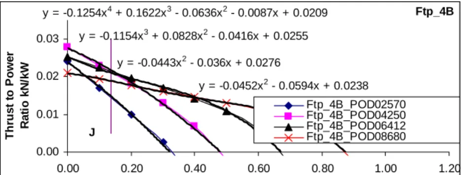
C7 and C10, thrust to power factors are plotted in the following figure, along with the

trend-line of each curve.

Ftp_4B y = -0.0452x2 _{- 0.0594x + 0.0238} y = -0.0443x2 - 0.036x + 0.0276 y = -0.1154x3 + 0.0828x2 - 0.0416x + 0.0255 y = -0.1254x4 _{+ 0.1622x}3 _{- 0.0636x}2 _{- 0.0087x + 0.0209} 0.00 0.01 0.02 0.03 0.00 0.20 0.40 0.60 0.80 1.00 1.20 J Th ru s t t o P o w e r Ra ti o k N /k W Ftp_4B_POD02570 Ftp_4B_POD04250 Ftp_4B_POD06412 Ftp_4B_POD08680

Figure 11. Plotting and creation of the thrust to power factor for the 4 pitch values at

different advance coefficient J.

Table 11 lists the thrust to power factors for each pitch value at each given speed. Values

in rows 3-6 in table are obtained by plugging the advance coefficient values to these

trend-line equations.

Table 11. Determination of thrust to power factor of the 4-blade propfan with the optimum pitch p/D of 0.6230

1 V

knots

23.00 24.00 25.00 26.00 27.00 28.00

2 J

0.1268 0.1323 0.1379 0.1434 0.1489 0.1544

p/D

3

0.0155 0.0151 0.0148 0.0144 0.0140 0.0136 0.2570

4

0.0223 0.0221 0.0218 0.0215 0.0213 0.0210 0.4250

5

0.0213 0.0212 0.0210 0.0209 0.0208 0.0206 0.6412

6

0.0191 0.0190 0.0189 0.0188 0.0187 0.0186 0.8680

7

0.0216 0.0214 0.0214 0.0212 0.0210 0.0209 0.6230

For each speed column, there are 4 factors corresponding to 4 different pitch values. The

thrust to power factor with the optimum pitch of p/D=0.6230 for the 4-blade propeller at

23 knots is obtained, as an example, by using the trend-line equation in the following

figure:

Figure 12. Thrust to power factor for different pitch values at 23 knots.

Plugging the optimum pitch value of p/D=0.6230 into the equation, the thrust to power

factor F

at 23 knots for the optimum pitch is obtained which is 0.0216.

The thrust to power factor for other speeds is obtained similarly. These plots and

trend-line equations are then used to obtain the thrust to power factor F

at other speeds (see

the last row of table 11).

To estimate the required power for the 4-blade propfan with the optimum pitch at 25

knots, there needs:

1. The thrust to power factor F

at 25 knots and from table 11, it is 0.0214.

2. The thrust requirement at 25 knots, T=R/(1-t) and from the trend-line equation in

figure 9, it is 3.6017 kN.

Therefore, the required power is T/F

=3.6017kN/0.0214 kN/kW =168 kW. With the

consideration of Mach number and shaft transmission efficiency, the required engine

power is then 168/0.9/0.98=190 kW. This is close to the value in row 25 of table 10,

which is 186 kW.

2.5 Propeller blade strength estimation

Strength estimation is based on the following assumptions:

• The material is carbon fiber composite.

• The maximum stresses occur at the blade root section, which is assumed at r/R = 0.3.

This is true as this was verified for all the output files for all J values of all

propellers.

• The blade root section in the propfan helical surface is assumed to be the blade

expanded plane on which the centroid and moment inertias were obtained.

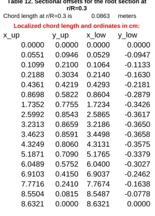
The sectional offsets for the r/R=0.3 section is list in table 12.

Table 12. Sectional offsets for the root section at r/R=0.3

Chord length at r/R=0.3 is 0.0863 meters

Localized chord length and ordinates in cm:

x_up y_up

x_low

y_low

0.0000

0.0000

0.0000

0.0000

0.0551

0.0946

0.0529

-0.0947

0.1099

0.2100

0.1064

-0.1133

0.2188

0.3034

0.2140

-0.1630

0.4361

0.4219

0.4293

-0.2181

0.8698

0.5822

0.8604

-0.2879

1.7352

0.7755

1.7234

-0.3426

2.5992

0.8543

2.5865

-0.3617

3.2313

0.8659

3.2186

-0.3650

3.4623

0.8591

3.4498

-0.3658

4.3249

0.8060

4.3131

-0.3575

5.1871

0.7090

5.1765

-0.3379

6.0489

0.5752

6.0400

-0.3027

6.9103

0.4150

6.9037

-0.2462

7.7716

0.2410

7.7674

-0.1638

8.5504

0.0815

8.5487

-0.0778

8.6321

0.0000

8.6321

0.0000

Figure 12 shows the plotted sectional shape for r/R=0.3.

-0.6 -0.3 0.0 0.3 0.6 -4.0 -3.0 -2.0 -1.0 0.0 1.0 2.0 3.0 4.0 5.0 X Z

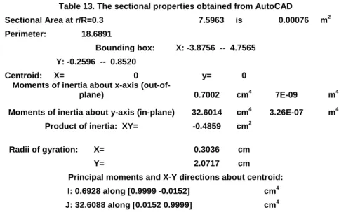
For this section, moments of inertia along with other geometry parameters were obtained

from with AutoCAD by using the MassProp command for a polyline-drawn and

Region-ized sectional offsets. The sectional properties are listed in the following table:

Table 13. The sectional properties obtained from AutoCAD

Sectional Area at r/R=0.3 7.5963 is 0.00076 m2

Perimeter: 18.6891

Bounding box: X: -3.8756 -- 4.7565 Y: -0.2596 -- 0.8520

Centroid: X= 0 y= 0

Moments of inertia about x-axis

(out-of-plane) 0.7002 cm4 7E-09 m4

Moments of inertia about y-axis (in-plane) 32.6014 cm4 3.26E-07 m4

Product of inertia: XY= -0.4859 cm2

X= 0.3036 cm

Radii of gyration:

Y= 2.0717 cm

Principal moments and X-Y directions about centroid:

I: 0.6928 along [0.9999 -0.0152] cm4

J: 32.6088 along [0.0152 0.9999] cm4

The following table lists the values needed for stress calculation.

Table 14. Values needed for stress calculation Out-of-plane bending about x-axis:

Cy_compress= 0.6831 cm 0.00683100 meters

Cy_tensile -0.5486 cm -0.00548600 meters Moment of inertia about x-axis I_x= 0.00000001

Out-of-plane bending moment coefficient

-0.00749400 N-m

In-plane bending about y-axis:

Compressive stress = moment*Cx_compress/I_y

Tensile stress = moment*Cx_tensile/I_y

Cx_compress= 4.7565 cm 0.04756500 meters

Cx_tensile -3.8756 cm -0.03875600 meters Moment of inertia about y-axis I_y= 0.00000033

In-plane bending moment: coefficient, in N-m

and safety factor 0.00133100 N-m

Spindle torque about the centroid

Tortional shear stress = torque*Cr/I_r Cr= 0.061355169 meters I_r= 3.260892E-07 m4 Spindle torque: coefficient

0.00042700 N-m

With the values in table 14 and the formulae for stress calculation, and some propfan

motion information, stresses and safety factors are ready to be obtained. The information

is:

• Diameter of the propeller D =1.4732 m

• Revolution speed n = 63.3333 rps

• Air density ρ = 1.225 kg/m

• The moment and torque factor = ρn

_D

_{= 34092.8741}

• Assumed carbon fibre composite ultimate tensile stress in bending: 4.47E+08 N/m

• Assumed ultimate compressive stress in bending: 4.78E+08 N/m

• Assumed ultimate tortional shear stress in tortional deformation: 9.28E+07 N/m

With the information above, stresses due to bending moments (blade root section in-plane

and out-of-plane) and the tortional stress due to blade root section spindle torque, along

with the safety factors, are listed in the following table.

The formulae for calculating the stresses are bending moment about x and y axis and

tortional stress about the normal vector to the section pass though the centroid:

,

I

C

M

=

σ

(17)

,

I

C

M

=

σ

(18)

,

I

I

C

+

=

τ

σ

(19)

and safety factor

Stress

Allowable

Stress

Ultimate

F

S

.

.

=

.

(20)

Table 16. Stresses and safety factor calculation

4-blade 6-blade 8-blade

Out-of-plane N-m -255.492 Safety factor Out-of-plane N-m -219.15 Safety factor Out-of-plane N-m -193.4 Safety factor Compress -2.49E+08 1.9177 Compress -2E+08 2.2358 Compress -2E+08 2.5329 Tensile 2.00E+08 2.2330 Tensile 171701141 2.6034 Tensile 1.52E+08 2.9493 In-plane N-m 45.377616 Safety factor In-plane N-m 33.0701 Safety factor In-plane N-m 25.638 Safety factor Compress 6.62E+06 72.199 Compress 4824881 99.07 Compress 4E+06 127.79 Tensile -5.39E+06 82.8634 Tensile -4E+06 113.7 Tensile -3E+06 146.66

Spindle N-m 14.557657 Safety factor Spindle N-m 11.3529 Safety factor Spindle N-m 9.2733 Safety factor Tortional shear 2.74E+06 33.8798 Tortional shear 2136105 43.444 Tortional shear 2E+06 53.186

The data in table 16 is divided into 9 blocks. They are for blade number of 4, 6 and 8 with

the stresses and safety factors for out-of-plane, in-plane moments and spindle torque.

2.6 Summery of the propeller geometry and configuration

A summary is listed in table 11.

Table 11. Summary of the propfan and configuration for the

4-bale propfan

Number of propfans

2

Ship speed (knots)

25.0000

Ship speed (m/s)

12.8625

Advance coefficient J

0.1379

Number of blades

4

6

8

Nominal p/D at r/R=0.75

0.6230

0.4926

0.4213

Pitch angle (rad)

0.2585

0.2061

0.1769

Pitch angle (deg)

14.8097 11.8089 10.1376

Pitch angle adjustment (reference

to the aligned dots)

4.5853 1.5845 -0.0868

Achievable efficiency

0.2818

0.2621

0.2294

Required engine power kW

187

201

230

Required engine power HP

254

273

312

Safety factor for compressive

stress (on the blade suction side)

due to out-of-plane bending

moment

3 CONCLUDING

REMARKS

3.1 Uncertainty remarks

There are a number of items that could affect uncertainty, such as the following:

• The accuracy of the geometry data measurement. The geometry data was obtained by a

laser scanning machine performed by IOT Design and Fabrication. Machine

precision and human related conversion/reading errors could cause some degree of

uncertainty, though these should be small enough to be neglected.

• The accuracy of the code. Though PROPELLA has been verified and validated for

many propellers in many cases, there still exists uncertainty but it is deemed that

the predicted propulsion performance is accurate enough for this kind of design and

optimization.

• Estimated hub to diameter ratio is 0.3. This could be hydrodynamically conservative

which means that a smaller hub diameter in practice could give a higher efficiency

and hence lower required engine power. However, the safety factor of the blade

would be reduced.

• Compressibility also has an effect on the performance and the prediction was also

corrected.

• The ship hull efficiency is calculated based on a zero wake fraction factor and a zero

thrust deduction factor. These two factors are difficult to determine as the ship

travels in different terrains (on snow, ice, water, swamp, etc), it would have a

different values of each.

• The rotational speed has been assumed at 3800 RPM. This should be much lower at the

bollard-pull condition when the ship speed is zero. Assuming a higher value of

RPM at the bollard-pull condition, this would give a more conservative estimate of

the blade root section bending moment and spindle torque, and hence a

conservative estimate of blade strength.

3.2 Remarks on this design and optimization

The on-the-shell Warp Drive propeller blade has been extensively studied for its

aerodynamic propulsion performance. Design and optimization were performed based on

3 types of propeller configuration of 4, 6 and 8 blades. For each propeller type, the

optimum pitch was found for the maximum achievable efficiency and hence the

minimum required engine power. With a little sacrifice on strength allowance, the

4-blade propfan gives the best efficiency and lowest cost (fewer number 4-blades needed to

be purchased).

It is important to make sure a correct pitch value can be obtained when adjusting the pitch

angle. The pitch angles referred to in this work have been based on the two marker dots

around the blade root section to align vertically.

With a little more work similar to the current study, a series of new propfans can be

developed specially for airboat propulsion. This current optimization and design has been

based on the given on-the-shelf Warp Drive propfan blade. This blade is primarily

designed and developed for much higher speeds in applications of hovercrafts or

Wing-in-ground ships. These speeds are usually over 100 mp/h (approximately over 160 km/h,

or about 70 m/s). The airboat in this work travels typically a lot less, at about 13 m/s.

This means that a very lightly loaded propeller blade and configuration have been used

for a very heavily loaded condition. There should be substantial room to improve the

propulsion performance by developing a series of propellers/propfans especially for

airboat.

The current Warp Drive propeller has a nearly constant maximum sectional thickness and

shape across the span. Therefore, the allowable strength of the propeller blade could

reach a substantially higher level by increasing the thickness and area of the blade root

section.

ACKNOWLEDGEMENT

The author thanks the National Research Council Canada for its support. Mr. Tony

Randell at IOT Design and Fabrication is acknowledged for geometry data measurement

and scanned images for this work. Mr. Derek Yetman is also appreciated for his

continuing assistance in proofreading various publications.

REFERENCES

Fred E. Weick, 1938. “Working charts for the selection of Aluminum alloy propellers of a

standard form to operate with various aircraft engines and bodies,” NACA Report No.

350. 16p.

David Biermann and Edwin P. Hartman, 1938, “The effect of compressibility on eight

full-scale propellers operating in the take-off and climbing range,” NACA Report No.

639. pp. 517-545.

Edwin P. Hartman and David Biermann, 1938, “The aerodynamic characteristics of

full-scale propellers having 2, 3, and 4 blades of Clark Y and R.A.F. 6 airfoil sections,”

NACA Report No. 640. 24p.

David Biermann and Edwin P. Hartman, 1938, “Tests of five full-scale propellers in the

presence of a radial and a liquid-cooled engine nacelle, including tests of two spinners,”

NACA Report No. 642. pp. 589-615.

Pengfei Liu, 2003. “PROPELLA Manual”, Institute for Ocean Technology, National

Research Council Canada, 56 p.

4 APPENDIX A: PREPARATION OF SECTIONAL

OFFSETS DATA

Table A1. Original measured data with some necessary smooth

X (%) X (value) Z (Upper) Z (Lower)

0.000 0 0.107 0.107 0.625 0.02271875 0.1522 0.0706 1.250 0.0454375 0.1746 0.0454 2.500 0.090875 0.2104 0.0421 5.000 0.18175 0.2678 0.0247 10.000 0.3635 0.3456 0.0103 20.000 0.727 0.423 0.0016 30.000 1.0905 0.4444 0.0002 31.200 1.1352 0.4447 0 40.000 1.454 0.4367 0 50.000 1.8175 0.409 0 60.000 2.181 0.3648 0.0022 70.000 2.5445 0.3081 0.0053 80.000 2.908 0.2408 0.0104 90.000 3.2715 0.1642 0.0174 99.200 3.6069 0.0876 0.0252 99.300 3.6102 0.0868 0.0259 100.000 3.635 0.0564 0.0564

Table A2. Rotation for Base-line to Nose-tail conversion

rad deg

angle= -0.01391932 -0.79751835 x_int_up z_int_up x_int_lo z_int_lo -0.00148932 0.10698963 -0.00148932 0.10698963 0.0205981 0.15250148 0.02173388 0.07090938 0.04300286 0.17521552 0.04480118 0.04602804 0.08793767 0.2116445 0.09028021 0.0433608 0.17800492 0.27030381 0.1813886 0.02722736 0.35865442 0.35062603 0.36332142 0.01535851 0.72104189 0.43307804 0.7269073 0.01171886 1.08420881 0.45953548 1.09039158 0.01537851 1.12890031 0.46045762 1.13509003 0.0158007 1.44778078 0.45689574 1.45385915 0.02023804 1.81163112 0.43425793 1.81732393 0.02529755 2.17571112 0.39512172 2.1807581 0.03255685 2.5399651 0.34348672 2.54417974 0.04071606 2.90436663 0.28125275 2.90757354 0.05087507 3.2688976 0.20971968 3.27094089 0.0629339 3.6053313 0.13779549 3.60619984 0.07540154 3.60864211 0.1370415 3.60948977 0.0761474 3.63386285 0.10698963 3.63386285 0.10698963

Table A3. NACA sectional format

r= 17" r/R= 0.5862069 x_new_up z_new_up x_new_lo z_new_lo

0.0000 0.0000 0.0000 0.0000 0.6076 1.2519 0.6388 -0.9925 1.2239 1.8767 1.2733 -1.6769 2.4599 2.8788 2.5244 -1.7503 4.9375 4.4924 5.0305 -2.1941 9.9067 6.7019 10.0351 -2.5206 19.8751 8.9699 20.0365 -2.6207 29.8650 9.6977 30.0351 -2.5200

31.0944 9.7231 31.2646 -2.5084 39.8660 9.6251 40.0332 -2.3863 49.8747 9.0024 50.0313 -2.2472 59.8897 7.9258 60.0285 -2.0475 69.9094 6.5055 70.0254 -1.8230 79.9333 4.7936 80.0215 -1.5436 89.9607 2.8259 90.0169 -1.2119 99.2152 0.8474 99.2391 -0.8689 99.3062 0.8267 99.3296 -0.8484 100.0000 0.0000 100.0000 0.0000

Table A4. Original measured data with some necessary smooth

X (%) X (value) Z (Upper) Z (Lower)

0 0 0.1205 0.1205 0.625 0.0224375 0.1605 0.0838 1.25 0.044875 0.1824 0.0673 2.5 0.08975 0.2183 0.0455 5 0.1795 0.2708 0.0225 10 0.359 0.3408 0.0082 20 0.718 0.4128 0.001 30 1.077 0.4374 0 32.3 1.1617 0.4383 0 40 1.436 0.4312 0 50 1.795 0.4043 0 60 2.154 0.3607 0 70 2.513 0.3036 0 80 2.872 0.2408 0 90 3.231 0.1505 0 99.1 3.5588 0.0637 0 99.4 3.567 0.0614 0.0011 100 3.59 0.0312 0.0312

Table A5. Rotation for Base-line to Nose-tail conversion

rad deg

angle= -0.02486952 -1.42491873 x_int_up z_int_up x_int_lo z_int_lo -0.00299647 0.12046274 -0.00299647 0.12046274 0.01843941 0.16100832 0.02034671 0.08433204 0.04032539 0.1834595 0.04318758 0.06839509 0.08429379 0.2204643 0.0885908 0.04771774 0.17271052 0.27517988 0.17888499 0.02695666 0.35041433 0.34962185 0.35868508 0.0171247 0.70751289 0.43052683 0.71775311 0.01885417 1.06579015 0.46404646 1.07666696 0.02678172 1.15044158 0.46705241 1.16134077 0.02888795 1.42483331 0.46677561 1.43555594 0.03570895 1.78439122 0.44881117 1.79444493 0.04463619 2.1443644 0.41415189 2.15333392 0.05356343 2.50467329 0.36599679 2.5122229 0.06249067 2.86512393 0.31214345 2.87111189 0.07141791 3.2262584 0.23079861 3.23000088 0.08034515 3.55611548 0.15217684 3.55769951 0.08849654 3.56437014 0.15008146 3.56586962 0.08980011 3.58811401 0.12046274 3.58811401 0.12046274

Table A6. NACA sectional format

r= 23” r/R= 0.79310345

x_new_up z_new_up x_new_lo z_new_lo 0.0000 0.0000 0.0000 0.0000 0.5969 1.1291 0.6500 -1.0061 1.2064 1.7542 1.2861 -1.4499

2.4307 2.7847 2.5504 -2.0257 4.8928 4.3083 5.0648 -2.6038 9.8413 6.3813 10.0716 -2.8776 19.7852 8.6342 20.0704 -2.8294 29.7620 9.5676 30.0649 -2.6087 32.1193 9.6513 32.4228 -2.5500 39.7601 9.6436 40.0587 -2.3601 49.7726 9.1434 50.0525 -2.1115 59.7966 8.1782 60.0463 -1.8629 69.8299 6.8373 70.0402 -1.6143 79.8672 5.3376 80.0340 -1.3657 89.9236 3.0725 90.0278 -1.1171 99.1090 0.8831 99.1531 -0.8901 99.3388 0.8248 99.3806 -0.8538 100.0000 0.0000 100.0000 0.0000

Table A7. Original measured data with some necessary smooth

X (%) X (value) Z (upper) Z (lower)

0 0 0.0626 0.0626 0.625 0.02088125 0.1016 0.0288 1.25 0.0417625 0.1217 0.0175 2.5 0.083525 0.1512 0.0066 5 0.16705 0.1975 0 10 0.3341 0.2617 0 20 0.6682 0.3281 0 30 1.0023 0.3509 0 34.3 1.1463 0.3531 0 40 1.3364 0.3493 0 50 1.6705 0.3244 0 60 2.0046 0.2816 0 70 2.3387 0.2301 0 80 2.6728 0.1692 0 90 3.0069 0.0961 0 99.2 3.315 0.0308 0 100 3.341 0 0

Table A8. Rotation for Base-line to Nose-tail conversion

rad deg angle= -0.01873471 -1.07341998

x_int_up z_int_up x_int_lo z_int_lo -0.00117272 0.06258901 -0.00117272 0.06258901 0.01897425 0.10197335 0.02033806 0.02918613 0.03947529 0.12246101 0.04142733 0.01827929 0.08067782 0.15273819 0.0833867 0.00816357 0.1633208 0.20059479 0.16702068 0.00312945 0.32913878 0.26791298 0.33404137 0.0062589 0.66193624 0.34056022 0.66808274 0.0125178 0.99555048 0.36961513 1.00212411 0.0187767 1.139484 0.37451238 1.14609884 0.02147435 1.32962182 0.37427431 1.33616548 0.02503561 1.66412966 0.35563758 1.67020684 0.03129451 1.99897283 0.31910399 2.00424821 0.03755341 2.33397898 0.27387193 2.33828958 0.04381231 2.66916122 0.21924152 2.67233095 0.05007121 3.00457202 0.15241325 3.00637232 0.05633011 3.31384126 0.09289654 3.31441825 0.06210194 3.34041369 0.06258901 3.34041369 0.06258901

Table A9. NACA sectional format

x_new_up z_new_up x_new_lo z_new_lo 0.0000 0.0000 0.0000 0.0000 0.6029 1.1786 0.6437 -0.9996 1.2164 1.7917 1.2748 -1.3260 2.4495 2.6978 2.5305 -1.6287 4.9226 4.1299 5.0333 -1.7794 9.8849 6.1445 10.0316 -1.6857 19.8441 8.3185 20.0281 -1.4984 29.8278 9.1880 30.0246 -1.3111 34.1352 9.3346 34.3331 -1.2304 39.8252 9.3275 40.0211 -1.1238 49.8357 8.7697 50.0175 -0.9365 59.8562 7.6764 60.0140 -0.7492 69.8815 6.3228 70.0105 -0.5619 79.9122 4.6880 80.0070 -0.3746 89.9496 2.6881 90.0035 -0.1873 99.2048 0.9070 99.2221 -0.0146 100.0000 0.0000 100.0000 0.0000

5 APPENDIX B: FINAL SECTIONAL OFFSETS FOR

PROPELLA INPUT

Table B1. Sectional Offsets at r/R=0.3

r= 8.7000” r/R= 0.3000 x_new_up Z_new_up x_new_lo z_new_lo

0.0000 0.0000 0.0000 0.0000 0.6385 1.0964 0.6133 -1.0966 1.2736 2.4331 1.2326 -1.3120 2.5353 3.5149 2.4796 -1.8878 5.0525 4.8881 4.9738 -2.5265 10.0759 6.7448 9.9680 -3.3358 20.1014 8.9836 19.9646 -3.9693 30.1104 9.8972 29.9643 -4.1899 37.4332 10.0316 37.2862 -4.2280 40.1102 9.9523 39.9651 -4.2376 50.1032 9.3374 49.9664 -4.1413 60.0908 8.2131 59.9688 -3.9140 70.0742 6.6636 69.9721 -3.5067 80.0542 4.8072 79.9769 -2.8519 90.0318 2.7921 89.9834 -1.8972 99.0541 0.9446 99.0342 -0.9018 100.0000 0.0000 100.0000 0.0000

Table B2. Sectional Offsets at r/R=0.4

r= 11.6000” r/R= 0.4000 x_new_up Z_new_up x_new_lo z_new_lo

0.0000 0.0000 0.0000 0.0000 0.6277 1.1507 0.6222 -1.0602 1.2562 2.2387 1.2469 -1.4395 2.5089 3.2927 2.4953 -1.8397 5.0123 4.7498 4.9936 -2.4104 10.0168 6.7298 9.9914 -3.0509 20.0224 8.9789 19.9897 -3.4981 30.0247 9.8275 29.9890 -3.6064 35.2183 9.9238 35.1822 -3.6271 40.0249 9.8379 39.9889 -3.5908 50.0233 9.2203 49.9891 -3.4794 60.0205 8.1127 59.9897 -3.2618 70.0166 6.6084 69.9907 -2.9184 80.0120 4.8025 79.9925 -2.3948 90.0069 2.8039 89.9951 -1.6577 99.1104 0.9106 99.1058 -0.8903 100.0000 0.0000 100.0000 0.0000

Table B3. Sectional Offsets at r/R=0.5

r= 14.5000” r/R= 0.5000 x_new_up Z_new_up x_new_lo z_new_lo

0.0000 0.0000 0.0000 0.0000 0.6169 1.2051 0.6311 -1.0239 1.2389 2.0443 1.2611 -1.5670 2.4826 3.0704 2.5109 -1.7917 4.9721 4.6116 5.0134 -2.2942 9.9577 6.7148 10.0149 -2.7661 19.9433 8.9741 20.0148 -3.0269 29.9389 9.7578 30.0138 -3.0230 33.0035 9.8160 33.0783 -3.0263 39.9396 9.7236 40.0127 -2.9439