Automated histopathological analyses at scale

Automated Histopathological Analyses at Scale

by

Mrinal Mohit

B. Tech., Indian Institute of Technology Kharagpur (2015)

Submitted to the Program in Media Arts and Sciences,

School of Architecture and Planning,

in partial fulfillment of the requirements for the degree of

Master of Science in Media Arts and Sciences

at the

MASSACHUSETTS INSTITUTE OF TECHNOLOGY

June 2017

Massachusetts Institute of Technology 2017. All rights reserved.

Signature redacted

Author ... ...

Program in Media Arts and Sciences

May 12, 2017

Signature redlact

C ertified by ...

Ramesh Raskar

Associate Professor

Program in Media Arts and Sciences

Thesis Supervisor

Accepted by...

MASSA 05MSNSTITUTE -OF TECHNOLOGY

JUL 3 1 Z017

>o

w

Pattie Maes

Academic Head

Program in Media Arts and Sciences

77 Massachusetts Avenue Cambridge, MA 02139

MIT~ibranes

http://Iibraries.mit.edu/ask

DISCLAIMER NOTICE

Due to the condition of the original material, there are unavoidable flaws in this reproduction. We have made every effort possible to provide you with the best copy available.

Thank you.

Some pages in the original document contain text that runs off the edge of the page.

Automated Histopathological Analyses at Scale

by

Mrinal Mohit

Submitted to the Program in Media Arts and Sciences, School of Architecture and Planning,

on May 12, 2017, in partial fulfillment of the requirements for the degree of

Master of Science in Media Arts and Sciences

Abstract

Histopathology is the microscopic examination of processed human tissues to diag-nose conditions like cancer, tuberculosis, anemia and myocardial infractions. The diagnostic procedure is, however, very tedious, time-consuming and prone to misin-terpretation. It also requires highly trained pathologists to operate, making it un-suitable for large-scale screening in resource-constrained settings, where experts are scarce and expensive.

In this thesis, we present a software system for automated screening, backed by deep learning algorithms. This cost-effective, easily-scalable solution can be operated by minimally trained health workers and would extend the reach of histopathological analyses to settings such as rural villages, mass-screening camps and mobile health clinics. With metastatic breast cancer as our primary case study, we describe how the system could be used to test for the presence of a tumor, determine the precise location of a lesion, as well as the severity stage of a patient. We examine how the algorithms are combined into an end-to-end pipeline for utilization by hospitals, doctors and clinicians on a Software as a Service (SaaS) model. Finally, we discuss potential deployment strategies for the technology, as well an analysis of the market and distribution chain in the specific case of the current Indian healthcare ecosystem.

Thesis Supervisor: Ramesh Raskar

Automated Histopathological Analyses at Scale

by

Mrinal Mohit

The following people served as readers for this thesis:

Thesis Reader ...

_r

Edward Boyden

Associate Professor of Media Arts and Sciences

Program in Media Arts and Sciences

Thesis Reader ...

(

Sepandar Kamvar

Associate Professor of Media Arts and Sciences

Program in Media Arts and Sciences

Acknowledgements

I am grateful to my advisor, Prof. Ramesh Raskar, for his continued support, guid-ance and mentorship. His suggestions, advice and feedback on the project have been invaluable for the work presented in this thesis.

I also thank the Camera Culture group at the MIT Media Lab, especially Anshu-man Das, Tristan Swedish and Otkrist Gupta, for their invigorating discussions and helpful inputs.

This work uses publicly available datasets graciously collected and hosted by the Rad-boud University Medical Center and Utrecht University Medical Center, Netherlands.

This work was funded by the MIT Tata Center for Technology and Design and the MIT Media Lab consortium.

Contents

Abstract

1 Introduction:

1.1 Motivation . . . . 1.2 Contributions . . . . 2 Background and Related Work:

2.1 Digital Pathology . . . . 2.2 Classical Computer Vision . . . . 2.3 Deep Learning . . . . 3 Algorithms for Lesion Classification:

3.1 D ataset . . . . 3.2 Evaluation Metrics . . . . 3.3 Classification Pipeline . . . . 3.3.1 Pre-processing . . . . 3.3.2 Data Augmentation . . . . 3.3.3 Patch-based Classification . . . . 3.3.4 Post-processing of likelihood maps . . . 3.4 Results and Discussion . . . . 4 Algorithms for Lesion Localization:

4.1 Evaluation Metrics . . . . 4.2 Two-stage thresholding model . . . . 4.3 Localization as Regression . . . . 4.4 Region Proposal Network . . . . 4.5 Results and Discussion . . . . 5 Algorithms for Patient Stage Determination: 5.1 D ataset . . . . 5.2 Evaluation Metrics . . . . 5.3 Rule-based approach . . . . 5.4 Joint Learning of slide label and pN stage . .

3 14 14 15 19 19 20 21 23 23 24 26 26 30 31 36 36 40 40 41 43 46 47 49 49 50 51 53

5.5 _{Results and Discussion . . . . 54}

6 Analysis of Deployment Strategies: 56 6.1 _{Quantified Value Articulation . . . . 56}

6.1.1 _{Channels. . . . . 60} 6.1.2 _{Revenue Streams . . . . 60} 6.1.3 _{Cost Structure . . . . 61} 6.2 _{Customer Segments . . . . 62} 7 Conclusions: ₆₅ 7.1 _{Summary . . . . 65} 7.2 _{Future Work. . . . . 67}

List of Figures

1-1 Lymph nodes are small glands that filter lymph, a colorless fluid con-taining white blood cells that bathes the tissues and drains through the lymphatic system into the bloodstream. Metastatic involvement of lymph nodes is one of the most important prognostic factors in breast cancer. They are surgically removed and examined microscopically, as in the whole-slide images analyzed in the following chapters. (Illustra-tion adapted from the Na(Illustra-tional Breast Cancer Founda(Illustra-tion [21]) . . . 16

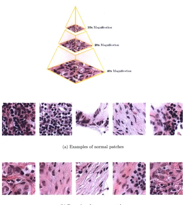
3-1 A typical whole-slide scanner system (courtesy of OptraScan [47]). These solutions can scan over 120 slides at once, with the option of 10x, 20x or 40x magnification. The output is usually in multi-resolution TIFF image pyramids and of resolutions in the order of 200,000 x 100,000 pixels at highest magnification. . . . . 24 3-2 Structure of a TIFF image pyramid file - the output of a whole slide

scanner. It usually is a 3 channel image over multiple optical resolu-tions (the highest magnification can reach 160 nm per pixel), for easy retrieval of relevant subregions. . . . . 25 3-3 Slide samples at highest magnification . . . . 25 3-4 Example of a whole-slide image with macro-metastases. The structures

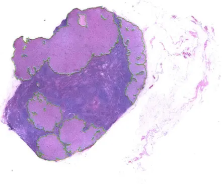
outlined in green represent the tumors in the sample (according to the pathologist-labeled ground truth annotations). At high magnification, the differences in local texture between the normal and metastatic regions. However, as later discussed, these differences can often be very subtle. . . . . 27 3-5 Results of background removal. The green lines delineate the regions

ultimately processed by the subsequent steps. On an average, 81% of the data is culled. . . . . 29 3-6 Architectures of popular deep convolution networks (Courtesy [29]) 35

3-7 Performance Characteristics on the Lesion Classification Task . . . . 37

3-8 Patch classification result sample 1. . . . . 38 3-9 Patch classification result sample 2. . . . . 39 4-1 Two-stage thresholding result sample. . . . . 42

4-2 Architecture of the Bounding Box Regressor Network. The final fully-connected layers in the original network are modified to introduce an

additional head trained with Euclidean loss. . . . . 43

4-3 The three stages of the localization-as-regression algorithm. . . . . 45

4-4 Schematic of the Fully Convolution structure of the RPN. . . . . 46

4-5 Performance Characteristics on the Lesion Localization Task . . . . . 48

5-1 Examples of lymph node sections with different metastasis classifica-tions (micro-metastasis top-left, macro-metastasis right, isolated tumor cells bottom-left). The extremely small size of micro-metastases and ITC on this zoom level illustrate the tediousness a pathologist faces while examining each small subregion at a higher magnification. . . . 52

5-2 Architecture for directly learning the pN stage of the patient from whole-slide images, rather than first explicitly learning the slide class lab el. . . . . 54

6-1 A business model canvas for deploying and commercializing the tech-nologies and algorithms described in the previous chapters . . . . 57 6-2 The collection center model for histopathological analyses in India. . 59

List of Tables

3.1 Performance of deep learning architectures . . . . 34

5.1 Metastasis classification rules . . . . 51

5.2 pN-stage classification system rules . . . . 53

5.3 Performance on the patient stage determination task . . . . 55

6.1 Breakdown of key customer segments . . . . 62

Chapter 1

Introduction

The field of pathology deals with providing clinical disease diagnoses to inform pa-tient treatment and management. Accurate and reproducible pathology diagnoses are essential for precision and targeted medicine. The primary tool used by pathologists has been the microscope, followed by a qualitative visual analysis [1] [39]. However, this has been limited by lack of standardized agreement between pathologists, as well as diagnostic errors arising from the task of manually analyzing gigapixel images for millions of cells across hundreds of slides on a daily basis [45] [49] [8], with inter-rater agreement sometimes as low as 48%, and only 70% on average. [17].

1.1

Motivation

As a case study for a particular pathology, we consider detecting metastatic breast cancer in digital whole slide images of lymph node biopsies. (Figure 1-1) According to the American Joint Committee on Cancer [16], a patient with sentinel lymph nodes diagnosed to be positive for breast cancer is assigned a more severe pathological

stage, with more aggressive interventions (like auxiliary lymph node dissection) than a patient with a negative result [43] [44] [3].

The manual visual analysis of sentinel lymph node slides is tedious, repetitive and laborious, especially for negative cases or cases with only very small affected regions. This often results in diagnostic errors and false negatives. Chemical alternatives for analysis like immunohistochemistry are limited by increased cost, increased processing and increased number of slides required, with little improvement in accuracy. [14]. The development of effective and cost-efficient computer-assisted image analysis sys-tems for lymph node evaluation remains an area of active research, as a high-performing system which could improve accuracy while reducing cognitive load would be highly valuable. [34]

In this thesis, we present a deep learning based approach for histopathological analy-ses, specifically identification and localization of breast cancer metastases from whole slide images of sentinel lymph nodes. We further study how these analyses from mul-tiple slides for a patient can be synthesized into an estimate of the clinical stage of the patient, and how these methods can be evaluated and compared to the state-of-the-art.

Additionally, we further present an analysis of how the algorithms can be combined into an end-to-end system for deployment, and what those deployment opportunities and challenges could be in the specific case of the Indian healthcare system.

1.2

Contributions

This thesis makes important contributions in showing how deep learning solutions can be used to automate histopathological analyses at scale, lowering cost and extending

Figure 1-1: Lymph nodes are small glands that filter lymph, a colorless fluid con-taining white blood cells that bathes the tissues and drains through the lymphatic system into the bloodstream. Metastatic involvement of lymph nodes is one of the most important prognostic factors in breast cancer. They are surgically removed and examined microscopically, as in the whole-slide images analyzed in the following chapters. (Illustration adapted from the National Breast Cancer Foundation [21])

Lymph Nodes

Tumor

Breast

-- -mmmmm~j / 4

(4

reach in resource-constrained settings. In the subsequent chapters, we describe in detail the following

-" Algorithms for identifying and classifying whole slide images of sen-tinel lymph nodes for metastatic breast cancer.

- A split-and-recombine strategy to train convolutional neural networks and employ them for localized predictive inference.

- An aggregation framework for post-processing likelihood maps into whole-slide classification results.

" Algorithms for precise automated localization of suspected tumor sites in whole slide images.

- A two-stage deep thresholding model which uses connected components in the likelihood maps to identify tumor locations.

- A region proposal network which learns to identify areas of potentially high information to guide search for tumor boundaries.

" Algorithms for synthesizing evaluations of multiple slides from differ-ent lymph nodes to characterize the clinical stage of a patidiffer-ent.

- A rule-based learner which incorporates guidelines followed by pathologists to rate clinical stage.

- A joint learning model for both likelihood and stage, which is able to encode information not captured by the guidelines.

" Analyses of deployment strategies for the software solution in India.

- A study of the key customer segments and stakeholders and promising business models in the Indian healthcare industry.

- An analysis of factors required to set up a sustainable platform and a chain for distribution.

Chapter 2

Background and Related Work

The conventional qualitative visual analysis for histopathological images relies on the digital imaging technologies employed to capture the relevant tissue image, and the expertise of the trained pathologist. The work presented in this thesis aims to present a number of methods to augment or enhance the latter component with computer vision and deep learning techniques. In this respect, this work draws from three broad areas - digital pathology, traditional computer vision and recent advances in deep learning. Following are key developments in each field which form the basis of this work.

2.1

Digital Pathology

Tissue samples for pathological analyses are usually collected via surgery or via biopsy, and need to be further processed in order to make glass slides which hold histological sections of the thickness of a few micrometers. This processing includes fixation, em-bedding, cutting and staining. During the preparation of histological slides, different

stains can be used for various purposes, but the hematoxylin and eosin (H&E) stain is most widely used; it induces sharp blue/pink contrasts across various sub-cellular structures and it is applied across many different tissue types.

Digital Imaging for pathology has gained acceptance in the last decade as the de facto representation modality, for easy access and archiving [23]. Whole-slide scanners are used to digitize glass slides at high resolution (up to 160nm per pixel). The availability of whole-slide images (WSI) has sparked the interest of the medical image analysis community, resulting in increasing numbers of publications on histopathological image analysis.

These whole-slide images are generally stored in multi-resolution TIFF pyramid files. Image files contain multiple down-sampled versions of the original image. Each image in the pyramid is stored as a series of tiles, to facilitate rapid retrieval of subregions of the image.

A typical whole-slide image is approximately 200,000 x 100,000 pixels on the highest resolution level with 3 byte RGB pixel format. This translates into over 56 GB of uncompressed pixel data from a single level. This has resulted in a need for clever techniques to efficiently handle and process such amounts of data.

2.2

Classical Computer Vision

Over the past decades, there has been an increased interest in computational methods for assistance in analysis of microscopy images in pathology. [27]

Historically, approaches to histopathological image analysis in digital pathology have focused primarily on low-level image analysis tasks (e.g., color normalization, nu-clear segmentation, and feature extraction), followed by construction of classification

models using classical machine learning methods, including: logisitic regression, sup-port vector machines, and random forests. Typically, these algorithms take as input relatively small sets of image features (10-100) [27] [32]. Further building on this framework, approaches have been developed for the automated extraction of moder-ately high dimensional sets of image features (1000s) from histopathological images followed by the construction of relatively simple, linear classification models using methods designed for dimensionality reduction, such as sparse regression [5].

2.3

Deep Learning

Since 2012, deep Convolution Neural Networks have significantly boosted accuracy on a wide range of computer vision tasks, including image recognition [38] [31] [52], object detection [25] [24] [50] and semantic segmentation [42]. They have also been employed productively in healthcare applications, notably detection of diabetic retinopathy from retinal fundus photographs [26], and dermatologist-level detection of melanoma from skin photographs [20].

In the context of histopathology, there have been studies in applying the above tech-niques to detect prostate cancer biopsies [41] and to segment epithelium, tubules, lym-phocytes, mitosis and lymphoma [35]. It has been demonstrated that CNNs achieved higher F1 score and balanced accuracy in detecting invasive ductal carcinoma.[13]. Mitosis detection competitions at ICPR 2012 [10] and AMIDA 2013 [61] have been won by teams which used CNNs. Predicting prognosis in non-small cell lung cancer using machine learning was described in [63]. In contrast to the types of machine learning approaches historically used in digital pathology, in deep learning-based ap-proaches there tend to be no discrete human-directed steps for object detection, object segmentation, and feature extraction. Instead, the deep learning algorithms take as input only the images and the image labels (e.g., 1 or 0) and learn a very

high-dimensional and complex set of model parameters with supervision coming only from the image labels.

It has been hypothesized that deep learning techniques could increase the sensitivity, speed and consistency of metastasis detection, but so far no systems have been able to deliver on those fronts to a clinically acceptable standard. [41]

Chapter 3

Algorithms for Lesion

Classification

Classifying whole-slide images of sentinel lymph node tissues extracted from suspected patients into normal or tumor is an important, and often critical, prognostic step for the pathologist. In this chapter, we describe the dataset we used to train our models on, the evaluation metrics to judge performance, the classification pipeline, and close with a discussion of the results.

3.1

Dataset

Whole-slide scanners (Figure 3-1) were used to collect images of sentinel lymph node tissues after fixation, embedding, cutting and staining by hematoxylin and eosin (H&E). These scanners can reach resolutions of upto 160 nanometer per pixel, and output images at multiple scanning resolutions in a pyramid structure (Figure 3-2). The data was collected by the Diagnostic Image Analysis Group (DIAG) and

Department of Pathology of the Radboud University Medical Center (Radboudumc) in Nijmegen, The Netherlands, and made available publicly in the Camelyon challenge

[22].

The data consists of a total of 400 whole-slide images of sentinel lymph nodes, split into a training set of 270 slides (160 normal, 110 tumor), and a test set of 130 slides. The ground truth data for the training slides consists of a pathologists delineation of regions of metastatic cancer on WSIs of sentinel lymph nodes. The data was provided in two formats: XML files containing vertices of the annotated contours of the locations of cancer metastases and WSI binary masks indicating the location of the cancer metastasis.

Figure 3-1: A typical whole-slide scanner system (courtesy of OptraScan [47]). These solutions can scan over 120 slides at once, with the option of 10x, 20x or 40x mag-nification. The output is usually in multi-resolution TIFF image pyramids and of resolutions in the order of 200,000 x 100,000 pixels at highest magnification.

3.2

Evaluation Metrics

The whole slide classification task between metastasis and normal slides is assessed by the means of the area under (AUC) the receiver operating characteristic (ROC) curve, which is a graphical plot that illustrates the performance of a binary classifier system

Structure of a TIFF image pyramid file - the output of a whole slide scanner. It usually is a 3 channel image over multiple optical resolutions (the highest magnification can reach 160 nm per pixel), for easy retrieval of relevant subregions.

lox Niuugliinfluii

Zft Magnificaion

40x Magniicaltion

-Ii

AlV

(a) Examples of normal patches

P &m 1

At

pt

A

1,4

Z . .0

16'V4

(b) Examples of tumorous patches

Figure 3-3: Slide samples at highest magnification Figure 3-2:

as its discrimination threshold is varied. It is created by plotting the true positive rate (TPR) against the false positive rate (FPR) at various threshold settings. The true-positive rate is also known as sensitivity or recall, while the false-positive rate is also known as the fall-out or probability of false alarm and can be calculated as (1 specificity). The ROC curve is thus the sensitivity as a function of fall-out

[4].

For each image in the test set, the algorithm ultimately provides the probability of that image to contain metastasis.

3.3

Classification Pipeline

Because of the extremely large size of each slide and the limited number of slides, we divide each whole-slide image into small square patches and train a deep convolutional neural network to make patch-level predictions to discriminate tumor-patches from normal-patches. We then aggregate the patch-level predictions to create tumor likeli-hood heatmaps and perform post-processing over these heatmaps to make predictions for the slide-based classification task (and later the tumor-localization task).

3.3.1

Pre-processing

The whole slide images invariably contain a lot of negative space (80%), which greatly increases computation time (with each image being 56 GB uncompressed). To re-duce the required compute and to focus on the regions most likely to contain cancer metastasis, we identify the tissue the image. This is achieved by an unsupervised thresholding process

-e Th-e imag-e is transform-ed from RGB to HSV cylindrical-coordinat-e color spac-e to reduce dependence of the procedure on lighting and contrast. The color (Hue, Saturation channels) is separated from the lighting (Value channel). [2]

Figure 3-4: Example of a whole-slide image with macro-metastases. The structures outlined in green represent the tumors in the sample (according to the pathologist-labeled ground truth annotations). At high magnification, the differences in local texture between the normal and metastatic regions. However, as later discussed, these differences can often be very subtle.

J

" Optimal threshold values are computed for each channel with Otsu's algorithm

for binary segmentation [48], which minimizes intra-class variance or equiva-lently, maximizes inter-class variance.

" A union is performed for the mask for H and S channels, and then its intersection with the original whole-slide image is taken as the new data source.

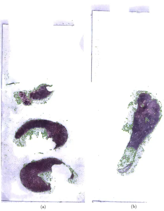
The reduction in area to consider is shown in Figure 3-5, with the threshold boundaries identified in green. On an average 81% of the data per whole-slide image is removed with this process, making subsequent steps computationally tractable.

We also perform stain specific standardization of the whole-slide images, analogous to that described in [6], to make the process invariant to most inconsistencies in the composition of the stain and the process of applying it. In order, we

1. Transform to the Hue-Saturation-Density space

2. Extraction samples for the hematoxylin, eosin and background classes from the WSI and derive the chromatic and density distributions of these classes.

3. Transform the 2D chromatic distribution for each dye class to match the chro-matic distribution of the corresponding class from a template slide.

4. Transform the density distribution for each dye class to match the density dis-tribution of the corresponding class from a template slide.

5. Weigh the contribution of stains for each pixel and obtain final chromatic and density transformations.

(a) (b)

Figure 3-5: Results of background removal. The green lines delineate the regions ultimately processed by the subsequent steps. On an average, 81% of the data is culled.

3.3.2

Data Augmentation

In order to further make the classifier robust to variance in orientation, stain color and other small perturbances, we augment our dataset with artificially generated samples

" We perform random translations by cropping a 224x224 subregion from the patch.

* We perform random horizontal flips and rotations by 90 degree multiples. " We perform random aspect ratio modifications in the range 3/4 to 4/3.

" We perform color perturbation by adding to the RGB channels multiples of their principal components, scaled by the eigenvalues times a normal random variable drawn from N(0, 1). i.e. to each RGB image pixel I,, = [Iv, I VG I XB]T we add the quantity

[PI, P2,i P31 [a1I-, a2'72, a37Y31,

where p and 7y are ith eigenvector and eigenvalue of the 3 x 3 covariance matrix of RGB pixel values, respectively, and a, is the aforementioned random variable. This scheme approximately captures an important property of natural images, namely, that object identity is invariant to changes in the intensity and color of the illumination.

" We add jitter to the patch extraction process so that each patch has a small x,y offset of up to 8 pixels.

The modifications are performed on-the-fly during training so that the transformed images need not be stored on disk, and sequenced on the CPU while the GPU is processing the last batch, severely reducing computational needs.

3.3.3

Patch-based Classification

The patch-based classification stage takes as input whole slide images (of resolution in the order of 200,000 x 100,000 pixels) and the ground truth image annotation delineating the locations of regions of each WSI containing metastatic cancer. We randomly extract millions of small (256 x 256 pixels) positive and negative patches from the set of training WSIs. If the small patch is located in a tumor region, it is a tumor

/

positive patch and labeled with 1, otherwise, it is a normal

/

negative patch and labeled with 0. On an average, we extract, without overlap, 1000 positive and 1000 negative samples from each tumor image (and only the latter from a normal images). This results in a total of 110,000 positive and 270,000 negative data points, representative samples of which are illustrated in Figure 3-4.

Following selection of positive and negative training examples, we use a deep neu-ral network to train a supervised classification model to discriminate between these two classes of patches. Deep learning enables a hierarchy of processing layers to au-tomatically learn representation of data with an increasing level of abstraction. It discovers intricate structure in large data sets by using the backpropagation algo-rithm to suggest how the computer should change its internal parameters that are used to compute the representation in each layer from the representation in the pre-vious layer. Deep convolutional networks have recently brought about breakthroughs in processing images, video, speech and audio. [40]

This is in sharp contrast to conventional machine-learning techniques which require careful engineering and considerable domain expertise to design a feature extractor that transformed the raw data into a suitable internal representation or feature vector from which the learning subsystem could detect patterns in the input. The key disadvantage of the using classical linear classifiers (which compute a weighted sum of the feature vector and compare it to a threshold) in the network is their limitation of

only being able to carve the input space into simple regions, i.e. half-spaces separated by a hyperplane. This works well for certain kinds of data but if applied to image recognition, it results in insufficient invariance to position, orientation or illumination. During the learning, the network (examples of the structure are described later), is shown an image patch and it produces an output probability for it being a tumor. The training dataset has images xi E RD, each associated with a label yi. Here i = 1... N

and yi 1 ... K. That is, we have N examples (each with a dimensionality D) and K distinct categories. The score function

f

: RD -+ RK maps the raw image pixels to class scores. An integral part of the multi-layered score function is regular non-linearities, which distinguish it from a linear classifier.

This score is unlikely to be correct before training. We compute a loss function that measures the error

/

distance between the output score and the desired score. We use the cross-entropy loss with weight decay, with each training example additively contributing Li =

fy,

+ log

Zj

efi, where

f

refers to the vector of class scores. Mini-mizing this loss is equivalent to miniMini-mizing the Kullback-Leibler divergence between the estimated class probability distribution and the underlying ground truth.

The network then adjusts its parameters (or weights) to reduce this error. The number of these weights are in the order of millions, and typically require millions of training examples to converge to a high enough accuracy. The adjustment of the weights is performed by computing the gradient of the error with respect to each weight, and then the weight is adjusted in the opposite direction, scaled by the learning rate 1. If performed over multiple layers, this results in the widely used backpropagation algorithm [30].

However, since computing the objective function over all the training examples could be very slow, Stochastic Gradient Descent (SGD) is used as an approximation. It divides the training data into a mini-batch of examples over which the gradient is

computed. Increasing the mini-batch size trades off frequency of update for gradient accuracy and smoothness

[7],

but in practice having hundreds of examples in a batch is sufficient for a reasonable gradient estimate. We initialize weights to small random numbers, accounting for the parameter count [28] and force activations throughout a network to take on a unit gaussian distribution at the beginning of the training (Batch Normalization [31]), along with L2 weight decay and dropout [58]). We further use the Adam optimization technique [36], modeled as

m = 01 * m + (1 - i1) * dx

v = 02 * v + (1 - 02) * dx2

where x is the gradient, m is the smoothened gradient, 1 is the learning rate, and

#1,

02 and c are hyperparameters. The trained network is finally run on a hitherto

unobserved test set (or in this case, a 15% validation set).

Convolutional architectures make the explicit assumption that the inputs are images, which allows us to encode certain properties into the architecture. These then make the forward function more efficient to implement and vastly reduce the amount of parameters in the network. The ones detailed in Figure 3-6 are composed of the following layers

* Input - holds the raw pixel values of the image, in this case an image of width 256, height 256, and with three color channels R,G,B.

" Convolution - computes the output of neurons that are connected to local re-gions in the input, each computing a dot product between their weights and a small region they are connected to in the input volume.

" MaxPool - performs a downsampling operation along the spatial dimensions (width, height)

" FC (fully-connected) - computes the final class scores.

We evaluate three deep learning network architectures for performing classification between the normal and the tumorous patches -VGG [55], Inception

[59]

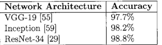
and Residual Networks [29]. The newly-introduced ResNets perform better than the previous state-of-the-art, as shown in Table 3.1

Network Architecture Accuracy

VGG-19 [55] 97.7%

Inception [59] 98.2%

ResNet-34 [29] 98.8%

Table 3.1: Performance of deep learning architectures

To bootstrap and learn from false positives, we extract additional negative samples from the non-tumor regions (200 per WSI) and retrain the model with the enhanced dataset.

Finally, we embed all the prediction (at stride 256) results into a likelihood (heatmap) image. Each pixel contains a value between 0 and 1, indicating the probability that the pixel contains tumor. Figure 3-8 and 3-9 present results of the patch classifica-tion on one of the whole-slide samples (with the overlaid annotated tumor) and the corresponding output likelihood map.

All experiments were performed with Torch [12] running on a server with 2x 8-core Intel Xeon E5-2620 A2.1 GHz, 128 GB DDR4 RAM, 2 TB SSD and 8x GTX 1080 8 GB. 8 replicas were run the GPUs with asynchronous gradient updates and batch size of 64 per replica. We used Adam [36] with c of 10-8, #1 of 0.9 and /2 of 0.999.

alit: 224 outut sie: 112 Output size: 51 Outu sine: Is output sine: 14 le: 7 WoE: I output size: 112 34-layer residual ImWe n64 /2 VGG-19 Imape PWa, /2 po, n Id co" 256 I Sd WNv 216 3p al, /2 3d mm, m1 pol, /2 Md UP, 512 Sd-ills li pool,/2 t "-fts I pWIt/2 t *2o | 35 (a) VGG-19 (b) ResNet-34 Output pool /2 size:56 _I conv,64 i ax cony, 64 3d m,64 an, 64 I3 con, 64 355 on, 64

output eize21 aim 126/

-sins: 28 ad mm, 128 d am, i28 Id aim, 123 dm, P121 'uso121 Output ouw, ize: 14ca,26 ad m'ISO Ad -, 256* _no 3d mmw, -3d mmco 266 3d - 266 as Mum ,i Unv62M MIleedm, 32 output ... ... [u: I sn/2

I A".M Ili -se jna

.d IeM, I Output

oeep"s

3.3.4

Post-processing of likelihood maps

We take as input a heatmap for each whole-slide image and produce as output a single probability of tumor for the entire WSI. We extract 28 geometrical and morphological features (skimage's regionprops [60]) from each heatmap, including the percentage of tumor region over the whole tissue region, the area ratio between tumor region and the minimum surrounding convex region, the average prediction values, and the longest axis of the tumor region. We compute these features over tumor probability heatmaps across all training cases, and we build a 50-tree random forest classifier to discriminate the WSIs with metastases from the negative WSIs.

On analyzing the relative importance of each feature, the following proved to be the most discriminatory

-1. With threshold = 0.5, the longest axis in the largest tumor region

2. With threshold 0.5, ratio of pixels in the region to pixels in the total bounding box (extent)

3. Eccentricity of the ellipse that has the same secondmoments as the region. (eccentricity)

4. Ratio of tumor region with threshold = 0.9 to the tissue region 5. With threshold = 0.5, the area of largest tumor region

3.4

Results and Discussion

We compared our classification receiver-operator characteristics to those previously considered-state-of-the-art. We test it against the performance obtained from support

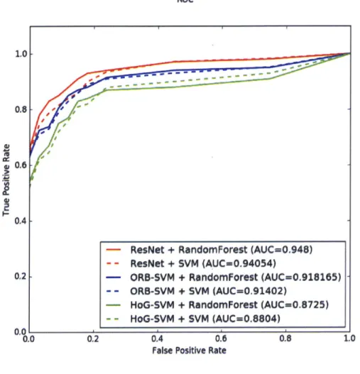
vector machines trained on Histogram of Oriented Gradients (HoG) [15] features and Oriented FAST and Robust BRIEF (ORB) [51] features of the input image data. The ROC curves in Figure 3-7 show how using a deep network boosted the AUC significantly.

Figure 3-7: Performance Characteristics on the Lesion Classification Task

ROC

1.0

0.8-0.6

0.4

- ResNet + RandomForest (AUC=0.948) - - ResNet + SVM (AUC=0.94054)

02 - ORB-SVM + RandomForest (AUC-0.918165)

- - ORB-SVM + SVM (AUC-0.91402)

- HoG-SVM + RandomForest (AUC=0.8725)

- - HoG-SVM + SVM (AUC=0.8804)

0.0 0.2 0.4 0.6 0.8 1.0

False Positive Rate

We also note that swapping out a random forest classifier in the post-processing step works better than a support vector machine, although not by much. We note that this metric is overall a challenging one because of the potential for false positives increases dramatically when a high level of patch-level predictions are obtained per slide. In contrast, human pathologist rarely demonstrate false positives in their analysis [35].

(md

(a) Whole-slide image with annotated tumors in green

(b) Tumor likelihood map generated by the patch classification stage. Since each pixel corresponds to a 256x256 patch in the original slide, the resolution is 65,000x lower.

Figure 3-8: Patch classification result sample 1.

/W

(t

(a) VWhole-slide im~age with aninotated tuniois in1 greenl

Chapter 4

Algorithms for Lesion Localization

The precise localization of lesions in a whole-slide image, especially of those that are very small in size is an important prognostic step, since the geometrical characteristics of the abnormality - like the size, eccentricity, location with respect to other cells etc., inform the diagnosis. It also is extremely tedious and laborious for the pathologist and is thus prone to errors. To explore a variety of methods to approach this task, we use the same dataset as described in the previous chapter.

4.1

Evaluation Metrics

The lesion localization performance is summarized using the Free Response Operating Characteristic (FROC) curve. This is similar to ROC analysis, except that the false positive rate on the x-axis is replaced by the average number of false positives per image. A true positive is considered if the location of the detected region is within the annotated ground truth lesion. If there are multiple findings for a single ground truth region, they are counted as a single true positive finding and none of them are

counted as false positive. All detections that are not within a specific distance from the ground truth annotations are counted as false positives. The final score is defined as the average sensitivity at 6 predefined false positive rates: 1/4, 1/2, 1, 2, 4, and 8 FPs per whole slide image.

For each tumor region detected in the whole-slide image (WSI), the algorithm provides the X and Y coordinates of the detected region together with a confidence score representing the probability of the detected region to be tumorous.

4.2

Two-stage thresholding model

We aimed to identify all cancer lesions within each whole-slide image with as few false positives as possible. We perform the pre-processing and patch classification steps described in Chapter 3, but proceed differently for the post-processing steps.

" We first train a deep model MA using our initial training dataset described in Chapter 3.

" We then train a second deep model MB with a training set that is enhanced with a higher representation of negative regions adjacent to tumors. This model

MB produces fewer false positives than MA but has reduced sensitivity.

" We threshold the heatmap produced from MA at TA, which creates a binary mask.

" We then identify connected components within the tumor binary mask, and we use the central point as the tumor location for each connected component. " To estimate the probability of tumor at each of these (x, y) locations, we take

the average of the tumor probability predictions generated by MA and MB

(a) Whole-slide image with annotated tumors in green

(b) Tumor likelihood map thresholded at TA. Since each pixel corresponds to a 256x256 patch in the origi-nal slide, the resolution is 65,000x lower.

(c) Centres of connected components in the thresholded

4.3

Localization as Regression

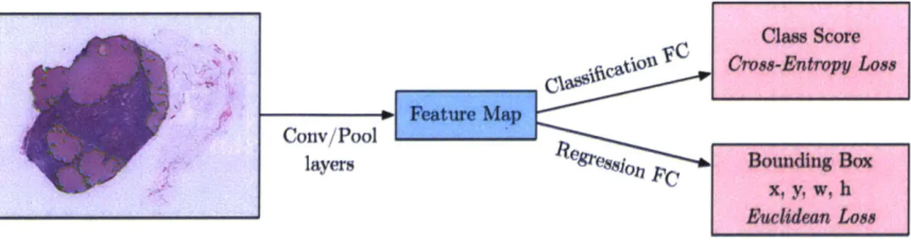
To explore if we can directly train the convolution network to predict boundaries of the tumor, we pose it as a regression problem for the location and size of their bounding boxes, which are then accumulated rather than suppressed in order to increase detection confidence. We apply this ConvNet at multiple locations in a sliding window fashion over multiple scales (4 here), which are then merged. The modified scheme for the network is shown in Figure 4-2. This method also avoids using background samples resulting in much faster training and side-stepping the bootstrapping process.

Figure 4-2: Architecture of the Bounding Box Regressor Network. The final fully-connected layers in the original network are modified to introduce an additional head trained with Euclidean loss.

Claw Score

UC

C f'stiou Cross-Entropy Loss Feature Map

Conv/Pool

layersegs.o 8 p Bounding Box

x, y, w, h

Euclidean Loss

To generate object bounding box predictions, we simultaneously run the classifier and regressor networks across all locations and scales. Since these share the same feature extraction layers, only the final regression layers need to be recomputed after computing the classification network. The output of the final softmax layer for a tumor at each location provides a score of confidence that a tumor is present (though not necessarily fully contained) in the corresponding field of view. Thus we can assign a confidence to each bounding box. Training the regressors in a multi-scale manner is important for the across-scale prediction combination. Training on a single scale will perform well on that scale and still perform reasonably on other scales.

However training multi-scale will make predictions match correctly across scales and exponentially increase the confidence of the merged predictions.

We combine the individual predictions via a greedy merge strategy applied to the regressor bounding boxes first introduced in [54].

1. Let C, be the set of classes in the top k for each scale s, found by taking the maximum detection class outputs across spatial locations for that scale.

2. Let B, be the set of bounding boxes predicted by the regressor network for each class in C,, across all spatial locations at scale s.

3. Let B = UsBs

4. Repeat until convergence:

* (b*, b*) = argminbj$b2 BMatchScore(b1, b2) * Stop, if MatchScore(b*, b*) > t.

* Else, let B = B\{b*, b;} U BoxMerge(b*, b*)

where MatchScore computes the sum of the distance between centers of the two bounding boxes and the intersection area of the boxes and BoxMerge compute the average of the bounding boxes coordinates. The final prediction is given by tak-ing the merged boundtak-ing boxes with maximum class scores, which is computed by cumulatively adding the detection class outputs associated with the input windows from which each bounding box was predicted. An example illustrating the pipeline is shown in Figure 4-3

AI

(a) Black rectangles mark the area under inspection at this scale, while red rectangles mark the predicted bounding box for that rectangle.

(b) High-confidence bounding boxes at multiple scale cluster around the tumors when visualized

(c) Greedy merging of theAoxes by confidence results in localization boxes for a particular scale.

4.4

Region Proposal Network

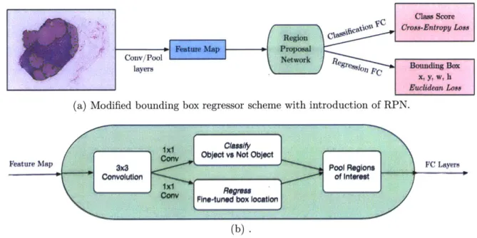
To further examine joint learning methods for the localization task, we evaluate a region proposal network (first introduced in [50]) to hypothesize object locations. A RPN is a fully convolutional network that simultaneously predicts object bounds and objectness scores at each position. Using the so-called "attention mechanism", the RPN component tells the unified network where to look.

The implementation is divided into two modules (Figure 4-4). The first module is a deep fully convolutional network that proposes regions and the second module is the detector described earlier in Section 4.3, which uses the proposed regions. To generate region proposals, we slide a small network over the convolutional feature map output by the last shared convolutional layer. This small network takes as input a 3 x 3 spatial window of the input convolutional feature map. Each sliding window is mapped to a lower-dimensional feature, which is fed into two sibling fully connected layers - a box-regression layer and a box-classification layer.

Class Score

hC5C3 Cross-Entropy Loss

Region

f.W Feature Map Proposal

Conv/Pool Network

layers Ressl Bounding Box

x, y, w, h

Euclidean Lose

(a) Modified bounding box regressor scheme with introduction of RPN.

1xI Cassif

Conv Object vs Not Object

Feature Map W .- Pool Regions FC Layers

Convolution of interest

N.- Regress

cov Fine-tunod box loostjon

(b).

This approach is translation-invariant, and can easily be extended to the multi-scale setting with a pyramid of anchors

[50].

However, we didn't observe significant boost in the performance by incorporating more than one scale - most of the discriminatory information for the pathology dataset appears to be at the highest magnification detail.

4.5

Results and Discussion

We compare the performance (Figure 4-5) of the three methods described above, along with a baseline of a very simple scheme of non-maxima supression which performs the following steps until convergence

-1. Take the maximum in the likelihood map as the probability of tumor in the entire image.

2. Set all values with a radius r of the maximum to 0.

The FROC metric is challenging because reporting multiple points per false positive region can significantly erode the score. We focused on the FROC as opposed to the AUC because there are approximately twice as many tumors as slides, which improves the reliability of the evaluation metric.

We also experimented with models pre-trained on ImageNet

[52]

which improved convergence speed in most cases, but failed to improve FROC, possibly due to the large difference in the kind of information present in the natural scenes of ImageNet vs the domain-specific pathology images, limiting the transferability.

Ensembling methods (averaging predictions from different augmentations, and aver-aging predictions of multiple independently-trained models) failed to provide a sig-nificant increase in the FROC score.

Figure 4-5: Performance Characteristics on the Lesion Localization Task Free response ROC

- RPN (0.7671)

- BoundingBox Regressor (0.7102)

- Two-Stage Thresholding (0.6981)

- Iterative Maxima (0.6797)

2 3 4 5

Average Number of False Positives

6 8 10 0.9 I- 1-0.7 0.6 IV S0.5 0.4 0.3 0.2 0.1 1-0.01₀ O.s 1-I

Chapter 5

Algorithms for Patient Stage

Determination

Moving from the detection and localization tasks described previously to patient-level analysis requires combining the detection and classification of metastases in multiple lymph node slides into one outcome: a pN-stage. This task has high clinical relevance and would normally require extensive microscopic assessment by pathologists of tens of slides per patient. An automated solution for assessing the pN-stage in breast cancer patients, would hold great promise to reduce the workload of pathologists, while at the same time, reduce the subjectivity in diagnosis.

5.1

Dataset

In addition to the whole-slide images of hematoxylin-and-eosin stained lymph node sections with lesion-level annotations, the dataset for patient-level analysis consisted of 5 lymph node slides each for 100 patients in the training set, and 5 lymph node

slides each for 100 patients in the test set, for a total of 1000 slides. Each slide had a corresponding severity stage (negative, micro-metastasis, macro-metastasis, isolated tumor cells (ITC)), but the ITC were not annotated exhaustively. Each patient had a corresponding pN stage label. This data was collected from 5 different laboratories by the providers and all ground-truth annotations were carefully prepared by expert-level pathologists [22].

In actual clinical practice, tens of lymph nodes are surgically removed and processed in the pathology laboratory. However, the size of the dataset would grow beyond rea-sonable size if all the slides were shared, hence the providers forged artificial patients, with 5 slides provided for each patient and each slide corresponding to exactly one node.

5.2

Evaluation Metrics

Internationally, the TNM system is widely accepted [57] as a means to classify the extent of cancer spread in patients with a solid tumour. It is one of the most important tools for clinicians to help them select the suitable treatment option and to obtain an indication of prognosis [9]. This prognosis usually worsens as the cancer spreads [53]. In breast cancer, TNM staging takes into account the size of the tumour (T), whether the cancer has spread to the regional lymph nodes (N), and whether the tumour has metastasised to other parts of the body (M). The dataset we had access to [22] focused on the pathologic N-stage (pN-stage) of the patients, which could be one of five classes.

Thus, the evaluation metric used was a five-class quadratic weighted Cohen's kappa coefficient, which measures inter-rater agreement with the pathologist provided ground truth. [11]

i= =k 1 -~

where k is the number of classes (pN-stages) and wij, xij, and mij are elements in the weight, observed, and expected matrices, respectively. The weights in the quadratic set are defined as:

W i = I - 2

(k - 1)2

The score is zero if the procedure does no better than random chance.

5.3

Rule-based approach

To compose a pN-stage, pathologists counts the number of positive lymph nodes (i.e. nodes with a metastasis). There are four categories a lymph node slide can be classified into:

Slide category Rule

Macro-metastases Metastases greater than 2.0 mm.

Micro-metastases _{Metastases greater than 0.2 mm or more than 200 cells,} but smaller than 2.0 mm.

Isolated Tumor Cells (ITC) Single tumor cells or a cluster of tumor cells smaller than 0.2 mm or less than 200 cells.

Negative None of the above.

Table 5.1: Metastasis classification rules

ITC is strictly not a metastasis and therefore lymph nodes containing only ITC are not counted as positive lymph nodes. However, pathologists are required to report on ITC when no macro-metastases or micro-metastases were found in a patient's lymph nodes.

Figure 5-1: Examples of lymph node sections with different metastasis classifications (micro-metastasis top-left, macro-metastasis right, isolated tumor cells bottom-left). The extremely small size of micro-metastases and ITC on this zoom level illustrate the tediousness a pathologist faces while examining each small subregion at a higher magnification. 'I-J

m

j

Q\

f

-~

I

~v.

)

A'

(

4 _

V

~1 -4'. 2.

A

4

F-i'

r

s

Pathologic lymph node classification (pN-stage) is then defined as in 5.2.

Patient Rule

category

pNO No micro-metastases or macro-metastases or ITCs found.

pNO(i+) Only ITCs found.

pNlmi Micro-metastases found, but no macro-metastases found. pN1 Metastases found in 1-3 lymph nodes, and at least one is a

macro-metastasis.

pN2 Metastases found in 4-9 lymph nodes, and at least one is a macro-metastasis.

Table 5.2: pN-stage classification system rules

This methodology is a simplified version of the official recommendations of the Union for International Cancer Control and the American Joint Committee on Cancer [46], due to lack of fine-grained data on lymph node's location of origin and molecular techniques like RT-PCR.

We modify our post-processing step defined in Section 3.3.4 to classify into 4 categories

- macrometasis, micrometastasis, ITC and negative, instead of just the two as earlier. We retrain the random forest classifer and then apply the rules as described above to get a final pN stage for the patient.

5.4

Joint Learning of slide label and pN stage

The pN stages provided in the dataset are consistent with the individual whole-slide labels, and the rules for determining the stage as described earlier. The rule-based approach's limitations are only (at least in this context) caused by imperfect classification into the four classes.

To explore the possibility of a model which bypasses the explicit step of learning the individual whole-slide label, and learns the pN stage directly from the

individ-Figure 5-2: Architecture for directly learning the pN stage of the patient from whole-slide images, rather than first explicitly learning the whole-slide class label.

Patient X Slide 11 CNN, Slide 2 CNN Slide 3 CNN, -pN Stage Slide 4A Feature Maps

ual slides, we restructure our network architecture (Figure 5-2) We run the patch-classification and recombination into heatmaps. as before, but now train a new deep network (ResNet-34) with each patient's 5 slides as a stacked input image of 5 chan-nels, to classify between the five pN stages. We boost the weight decay to avoid overfitting with the low number of examples.

5.5

Results and Discussion

We obtained the scores of Table 5.3 in the Cohen's Kappa evaluation metric. We note that the joint-learning approach boosted the score significantly, indicating that directly using the pN stage as the variable to be corrected reduced the build-up of errors from explicitly making an intermediate classification.

In particular, we also noted that the isolated tumor cells (ITC) were not exhaustively annotated in the ground truth set. If we replaced the labels of the slides marked as ITC to negative or to micro-metastases, we observe a minor improvement in perfor-mance.

Method K score r, score with r, score with

ITC as negative ITC as microm.

Joint-learning 0.8758 0.8921 0.8914

Rule-based approach 0.8386 0.8452 0.8435

Average Pathologist [17] 0.7 (Estimate) -

-Random Chance 0.0000 .0.0000 0.0000

Table 5.3: Performance on the patient stage determination task

between individual classes is unaccounted for. Moreover, the highly critical nature of detecting all positives, at some cost of false positives, can only be captured by ad-justing the weights accordingly. Nevertheless, the performance of the algorithms is a good indicator of the inter-rater agreement, which surpasses the average pathologist's score of 0.7 [17].

Chapter 6

Analysis of Deployment Strategies

An automated histopathological analysis platform could help the lives of millions of Indians who require screening and diagnostic services every year, by enabling a reduc-tion in reliance on hard-to-acquire experts, increase in throughput, and improvement in efficiency. It could be effectively deployed into the diagnostic pipeline of existing organized pathology lab chains, recuperating initial costs effectively over time while simultaneously getting better in terms of accuracy as access to more continuous data is made available. We present here a quantified articulation of a business model including activities, resources, customers, channels, costs, revenue streams and the value added.

6.1

Quantified Value Articulation

The healthcare industry amounts to over $80 billion in India, with over $1 billion directly coming from the domestic pathology market (growing at 20% compounded annual growth rate), mostly in Tier I cities [19]. This growth is heavily driven by

Figure 6-1: A business model canvas for deploying and commercializing the technologies and algorithms described in the previous chapters

Comm P1e9m-6a-ah I uch * DevulupueIf

For gLMing research by Bud voo--ncapt

pAn sanoles and technoogy into plnorm

MenAn

-

amcyingcurc APMMAW

~ ApdemTo pathology WEbs For enawing all testing hospamas, clnics and

and valldation foows government

legal-... .. ..

Bimrn Dmus

To buld the platform and

scile the tech.

SerVQrM

high-Pei rnrmnce nwdhins

and ~vk

Coot stnm*Ame

C Hstm maaareh/ bglinee

sihutluiS Od & Labelds

Whte ftrma Qdstm srnm w-"M cutmrSugmeni.

SOreaning Thfmaghp* Oa~tony tprviug Priinct Patmlgy eLabe

Increasing speed of Through learning from Prbmary adopters routine cbeckl by new data

providing fast preditionsesa

TechriAw SHOP at

uLow-cost screening For platform and tools makes more

Increasing eo. of people dlsrCINVnalve diagnoses with access to tech possible, could reduce

ou"PourSng

Seducad Rualance an xprts

Niftn Meedical Uftft

SCWn screening am... ...

augmenting a'State-sponsored last mile

rWOMW qwnda"ow 90rvkce

airedm SMS Con"Oh"Mn Quality

i To pathology lwbs and

Unlttdby dhoerse-- _clinics

-subjective opinions

s InotPartmarGhIAW

Through MU. SuMkes

etc

Seftwae esn -nitc