Computer Science and Artificial Intelligence Laboratory
Technical Report
m a s s a c h u s e t t s i n s t i t u t e o f t e c h n o l o g y, c a m b r i d g e , m a 0 213 9 u s a — w w w. c s a i l . m i t . e d u
MIT-CSAIL-TR-2014-003
March 16, 2014
An Architecture for Online
Affordance-based Perception and
Whole-body Planning
Maurice Fallon, Scott Kuindersma, Sisir
Karumanchi, Matthew Antone, Toby Schneider,
Hongkai Dai, Claudia PØrez D’Arpino, Robin Deits,
Matt DiCicco, Dehann Fourie, Twan Koolen, Pat
Marion, Michael Posa, AndrØs Valenzuela,
Kuan-Ting Yu, Julie Shah, Karl Iagnemma, Russ
Tedrake, and Seth Teller
An Architecture for Online Affordance-based
Perception and Whole-body Planning
Maurice Fallon, Scott Kuindersma, Sisir Karumanchi, Matthew Antone, Toby Schneider, Hongkai Dai, Claudia P´erez D’Arpino, Robin Deits, Matt DiCicco, Dehann Fourie,
Twan Koolen, Pat Marion, Michael Posa, Andr´es Valenzuela, Kuan-Ting Yu, Julie Shah, Karl Iagnemma, Russ Tedrake and Seth Teller
Computer Science and Artificial Intelligence Laboratory Massachusetts Institute of Technology
32 Vassar Street Cambridge, MA 02139
Abstract
The DARPA Robotics Challenge Trials held in December 2013 provided a landmark demon-stration of dexterous mobile robots executing a variety of tasks aided by a remote human operator using only data from the robot’s sensor suite transmitted over a constrained, field-realistic communications link. We describe the design considerations, architecture, imple-mentation and performance of the software that Team MIT developed to command and control an Atlas humanoid robot. Our design emphasized human interaction with an effi-cient motion planner, where operators expressed desired robot actions in terms of affordances fit using perception and manipulated in a custom user interface. We highlight several im-portant lessons we learned while developing our system on a highly compressed schedule.
1 Introduction
Since the start of the DARPA Robotics Challenge (DRC) in early 2012, we have worked as a team toward the realization of a software system for a human-scale robot that, given only limited communication with its human operators, can perform useful tasks in complex and unfamiliar environments—first in the simulation environment of the Virtual Robotics Challenge (VRC) in May 2013 and later in the physical DRC Trials. This paper describes the key ideas underlying our technical approach to the DRC, and the architecture that we adopted as we moved from conception to implementation. We elucidate several key components of our system—the human-robot interface, the perception, planning, and control modules, and the networking infrastructure—to illustrate how our approach met the requirements of the DRC Trials in December 2013. Finally, we look back on the previous two years both to give a sense of the experience of competing, and to draw useful lessons for the final DRC competition and for the field.
There are several key ideas behind our approach. The first is that, since the system includes a human operator in communication with the robot, the robot need not be fully autonomous. We chose to allocate the traditional executive (high-level task planning) functions to the operator, along with the responsibility to partition high-level plans into smaller “chunks” for autonomous execution by the robot. We aimed to encompass chunks of varying complexity, from small motions, such as would be executed by a conventional teleoperated robot, through primitive actions such as stepping, reaching, grasping and lifting, and finally to sub-tasks such as walking, fetching and using tools.
Our second key idea is to frame all operation of the robot in terms of operator-perceived affordances, or environmental features that hold possibilities for action (Gibson, 1977). We adopted an interface metaphor in which the operator first helps the robot perceive and interpret a task-salient affordance in its surroundings, then commands the robot to act in terms of this conveyed affordance. For example, to turn a valve, the operator first coarsely indicates the valve wheel in the currently available sensor data; the system responds by fitting a valve wheel template to this data. Once the operator is satisfied that the system has an actionable model of the valve wheel, s/he can command the robot to turn the valve. Templates can also incorporate valuable information provided by the system designers well in advance, such as manipulation stances or grasp locations likely to be successful. In this way our system factors some of the challenging and expensive aspects of online motion planning into an offline phase.
The third key idea is to combine optimization with human input. For perception, a human operator provides the rough morphology, location, and attitude of each affordance, after which the system uses optimization to fit parameters more precisely to sensor data. In footstep planning, the operator provides a goal and a maximum number of footsteps, and an optimizer fills in suitable footsteps given the terrain estimated by the perception system. In multi-contact planning, the human operator provides sequence points at which contacts are made and broken, mitigating the combinatorial complexity of algorithmic planning.
Beginning in March 2012, when we first heard that a new DARPA Challenge was being mounted, we gathered key people and system components. The lead PI (Teller) and co-lead (Tedrake) were joined by a perception lead (Fallon), a planning and control lead (Kuindersma), and a manipulation lead (Karumanchi). We incor-porated two key software modules from previous projects: LCM (Huang et al., 2010), a lightweight message-passing infrastructure and tool set for visualizing and logging streaming sensor data, and Drake (Tedrake, 2014), a powerful MATLAB toolbox for planning, control, and analysis using nonlinear dynamical systems. LCM was developed as part of MIT’s 2006-7 DARPA Urban Challenge (DUC) effort, and has since been released as open-source and used for a wide variety of projects both within and outside of MIT. Drake was initially developed by Tedrake and his research group to provide the planning and control infrastructure for numerous legged robot and UAV projects; we have now released this code as open-source as well.
DARPA’s timeline for the Challenge was highly compressed. Each team first had to choose the track in which to compete: Track A teams would develop both hardware and software, whereas Track B teams would develop software only, and upon successful qualification in a simulation environment, would receive a humanoid robot from DARPA. Excited by the opportunity to use a Boston Dynamics machine, we chose to compete as a Track B team.
Although our team brought considerable relevant experience to the project, we had very little direct exposure to humanoid robots. There were only 8 months between the kick-off meeting in October 2012—where we received our first draft of the rules—and the Virtual Robotics Challenge in June 2013; we subsequently received our Atlas robot on August 12, 2013, and had to compete again, this time with the real robot, only four months later. In this brief period, we developed substantial components of our system from scratch (including, for instance, an optimization-compatible kinematics and dynamics engine, and a complete user interface) and integrated complex existing software. Many of us made considerable personal sacrifices for the project, devoting countless hours because we believed it was an incredible and unique opportunity.
2 Overview of the Atlas Robot
Atlas is a full-scale, hydraulically-actuated humanoid robot manufactured by Boston Dynamics. The robot stands approximately 188cm (6ft 2in) tall and has a mass of approximately 155kg (341lb) without hands attached. It has 28 actuated degrees of freedom (DOFs): 6 in each leg and arm, 3 in the back, and 1 neck joint. A tether attached to the robot supplies high-voltage 3-phase power for the onboard electric hydraulic pump, distilled water for cooling, and a 10Gbps fiber-optic line to support communication between the robot and field computer. Despite its considerable size, the robot is capable of moving quickly due to its ability to
Figure 1: The platform consisted of the Atlas humanoid robot (left, photo credit: Boston Dynamics) which could be combined with a variety of hands or hooks via machined mounting plates. Right, clockwise: the iRobot and Robotiq hands, a hook for climbing, a 15cm wrist extender and a pointer for pushing buttons.
produce large forces (up to several hundred N-m in the leg joints) at high bandwidth.
Several sensor signals are available for integration with perception and control algorithms. Joint position, velocity, and force measurements are generated at 1000Hz on the robot computer and transmitted back to the field computer at 333Hz. Joint positions are reported by linear variable differential transformers (LVDTs) mounted on the actuators; velocities are computed through numerical differentiation of the position signals. Joint forces are estimated using pressure sensors in the actuators. In addition to the LVDT sensors, digital encoders mounted on the neck and arm joints give low-noise position and velocity measurements. A 6-axis IMU mounted on the pelvis produces acceleration and rotation measurements used for state estimation. Two 6-axis load cells are mounted to the wrists, and arrays of four strain gauges, one in each foot, provide 3-axis force-torque sensing.
Atlas has four primary behavior modes: balancing, stepping, walking, and user mode. The balancing mode provides basic dynamic balance capabilities where the pelvis pose and upper body DOFs are under operator control. The stepping behavior provides a basic walking capability that is driven by inputs specifying desired step locations and leg swing trajectories. The walking behavior is a faster and more dynamic locomotion mode, but because it is significantly less accurate and predictable than stepping, we did not use it in the DRC Trials. Finally, user mode puts all joint-level control under the command of the operator.
The Multisense SL sensor head was manufactured by Carnegie Robotics and consists of a stereo camera and a spindle-mounted Hokuyo UTM-30LX-EW planar lidar. Two PointGrey Blackfly cameras with 185-degree fisheye lenses were mounted on the upper torso for improved situational awareness. We also used a microphone located on the head to detect acoustic events (in particular drilling sounds).
2.1 Hands and End-Effectors
We used a variety of end-effectors that mounted directly onto the robot’s wrist force sensors (Figure 1). The rules of the competition allowed us to change end-effectors between tasks, so long as the robot carried all of its hands for all tasks. These included two types of actuated hands, the iRobot Dexter Hand and the Robotiq 3-Finger Adaptive Gripper. While the iRobot hand provided useful tactile sensing in its fingers and palm, the ruggedness of these sensors was unfortunately insufficient for our aggressive daily testing. We also used inert hooks and dowels in tasks that required large contact forces such as ladder climbing.
Figure 2: Visualization of the kinematic reachability of the robot from inferior (left), anterior (center), and medial (right) perspectives. We uniformly sampled 15 angles in the feasible range of each of the 6 right arm joints, divided the reachable workspace into 20 × 20 × 20 bins, and assigned each bin a score based on how many distinct end-effector orientations it contained.
2.2 Kinematic Reachabilty and Sensor Coverage
The robot’s arms have only six DOFs, its sensor head can pitch up and down but cannot yaw left and right. The arm kinematics and limited sensor head field of view played a role in shaping the solutions we devised to the manipulation problems faced in the trials. To obtain a rough idea of the robot’s manipulation “sweet spot,” we sampled 156 right-arm configurations, and rendered the end-effector workspace using isocontours
in Figure 2. Here red regions have the highest reachability score (∼75 distinct sampled orientations) and blue the lowest (∼5 or fewer distinct sampled orientations). In the right figure the horizontal field of view of the right head camera is shown.
One significant practical effect of limited reachability and sensor coverage on task development was that most object manipulation occurred outside the view of the high resolution head cameras. As a result, we were forced to rely heavily upon the low-resolution images produced by the situational awareness cameras and lidar. The relatively short length of the arms also made picking up objects on the ground while standing nearly impossible. We therefore opted to use 15 cm wrist extenders for the debris task, in which a longer reach was advantageous.
2.3 Kinematic calibration
Precise and accurate positioning of the end effector was a critical capability for many of the Trials tasks involving manipulation. Combined with high-fidelity perception, accurate reaching reduced or eliminated the need for manual adjustment of the end effector by the operator. To minimize forward kinematic error, we performed detailed calibration of the upper body joints. The arm and neck joints are each outfitted with two position sensors: a LVDT mounted on the actuator and a digital encoder on the linkage. Since the LVDTs are noisier and subject to up to two degrees of backlash in the linkage, we chose to calibrate the encoders and use them for forward kinematic positioning.
The kinematic calibration procedure of the n upper body joints was straightforward: VICON markers were placed on the upper torso of the robot and M markers on each of the end effectors. Data was collected from N different representative poses of the upper body. In the spirit of (Khalil and Dombre, 2004), and assuming that the initial calibration of the encoders was roughly correct, we then solved the unconstrained minimization problem: q∗= arg min qc∈Rn N X i=1 kφ(qi+ qc) − xik2, (1)
(a)
(b)
(c)
(d)
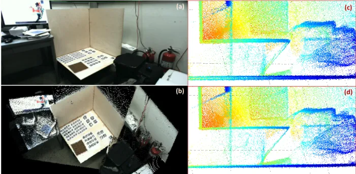
Figure 3: Head sensor calibration refinement. (a) Image of our calibration target acquired by the left head camera. (b) Post-calibration rendering of left head camera image projected onto lidar point cloud, demonstrating accurate alignment between laser and camera. (c) Side view of 360-degree lidar point cloud sweep before spindle calibration; flat surfaces (ground, target planes) appear doubled due to slight spindle misalignment. (d) Coherence of flat surfaces improves after spindle calibration.
where φ : Rn → R6M is the Cartesian position of the end effector markers, relative to the robot torso, as
predicted by the forward kinematics, qi∈ Rn are the measured, pre-calibration joint angles, and xi ∈ R6M
are the VICON measured marker positions.
The calibrated offset q∗ was then added to all encoder measurements to provide more accurate joint angle
estimation. This calibration procedure reduced forward kinematic error to roughly 0.5cm (from more than 3cm), although error was dependent on the specific robot pose.
Despite calibration, uncertainty remained in the absolute encoder positions after the robot was powered off and on. To account for this, the post-calibration positions of the encoders were measured and recorded at known joint limits. Upon robot start-up, an automated routine moved the joints to these known positions and updated the calibration data.
2.4 Perception calibration
Perception in the Trials primarily relied on (1) a pair of cameras in binocular stereo configuration mounted on the head; (2) a laser range scanner mounted on a rotating spindle on the head; and (3) a pair of wide-FOV cameras mounted on the chest. In order to place data from these sensors into a common reference frame for fusion and operator situational awareness, it was necessary to determine accurate geometric relationships among them.
The head stereo cameras and laser were factory calibrated, though we modified the rigid laser-to-spindle and spindle-to-camera transformations slightly to achieve better scan-to-scan and scan-to-scene consistency. This was achieved by collecting stereo depth maps and laser scans of a calibration target while rotating the spindle through 360 degrees. An optimization algorithm determined the transformations that minimized laser point dispersion on the three mutually distinct planar surfaces of the target (Figure 3).
(a) (b) (c)
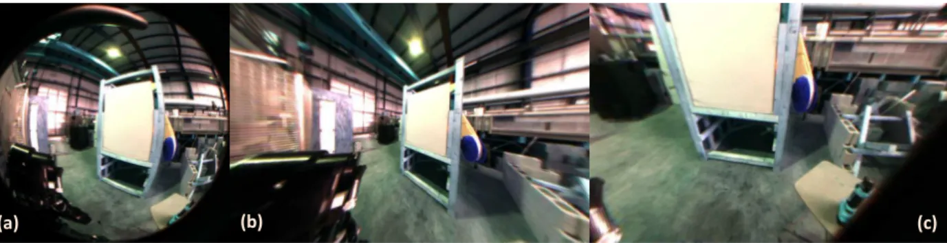
Figure 4: Fisheye lens rectification. (a) Raw image from left chest camera exhibits severe fisheye distortion and is difficult to interpret at the periphery. (b,c) After lens calibration, images can be rectified to produce arbitrary virtual viewpoints with minimal distortion.
(a) (b) (c)
Figure 5: Chest camera alignment. (a) SIFT feature matches extracted between head image (top) and left/right chest camera images (bottom) used to align the sensor frames. (b,c) Lidar points pseudo-colored by distance (top) and texture-mapped with chest camera images (bottom), demonstrating accurate alignment between head and chest data.
We determined each chest camera’s intrinsic lens parameters (focal length, projection center, and fisheye distortion profile) by applying a parameter-free radial calibration method to images of a known planar pattern, which enabled very accurate rectification over the entire field of view as well as synthetic planar projections that were more easily interpreted by the operator (Figure 4). We determined each camera’s extrinsic rigid pose with respect to the robot’s torso by first aligning them with the head, then inferring the camera-to-torso transformation via forward kinematics. The algorithm discovered SIFT feature matches between the head and chest cameras’ overlapping fields of view, and associated each matched feature with a laser return, thus producing a set of 3D-to-2D correspondences. A PnP (resection) solver wrapped in a RANSAC outer loop then used these correspondences to find a robust solution for the pose of each chest camera (Figure 5).
3 Software System Overview
The system we developed for the DRC Trials consisted mainly of software created during the simulation phase of the competition (Tedrake et al., 2014). Some components, such as the IK engine (Section 4.1) and height map software (Section 3.2.3), transferred to the physical robot without modification, while some task-specific planning interfaces, the model fitting interface (Section 5.1), and various controllers were developed
State Synchronization Multisense Head
and Chest Cameras Robot Hands
Map Collator and Server Image Snapshot & Compression Atlas Robot Controller Motion Planning
User Interface Affordance Server
Model Fitting User Interface
Candidate Plans
Joint Position and Velocity, Pelvis Pose Estimates (333Hz)
Joint Commands (333Hz) Raw Sensor Data
Committed Plans Compressed Range and Camera Imagery (On Request) Collated Robot State (4Hz)
Robot State and Perception Data Committed Plans
Planner Constraints
Restricted Link Operator Control Unit
Field Computer Components (via drivers and fiber)
Task Planners Footstep Planner Manipulation Planner
MIT Network Shaper MIT Network Shaper
Figure 6: The major software components of our system. A series of processes running on the robot collated kinematic and perception sensor data, and responded to operator requests for lidar and imagery (green). The operators interpreted this data (pink) and formulated motion plans (purple), which were executed by the robot controller (purple). Data was transmitted across DARPA’s restricted link by our network shaper software (ochre).
after the Atlas robot arrived.
Our multi-process software infrastructure involves modules communicating with one another in soft real-time using Lightweight Communication and Marshalling (LCM) message passing (Huang et al., 2010). LCM is implemented using UDP and supports a variety of language bindings, pairing well with our code base which was a heterogeneous mixture of C, C++, Python, Java and MATLAB. Communication contracts between processes were instantiated as LCM message definitions, which allowed independent development of modules. 3.1 System Layout
Our system architecture is illustrated in Figure 6 with its network layout defined by DARPA’s competition rules. The robot’s onboard computation resources were reserved for Boston Dynamics’ proprietary software, communicating over a 10 GB/s fiber-optic network with a series of field computers. This released teams from current computational constraints under the assumption that these field computers will eventually be transferred onto the robot in a future platform.
The human operators were separated physically from the robot (including the field computers) and had limited communication with it. Typically, two team members (one primary operator and one perception operator) interacted with the robot using standard Linux workstations that comprised the Operator Control Unit (OCU). Additional machines could be easily connected to the LCM network as required to monitor performance or run motion planners. LCM communication was unrestricted within the OCU and robot sub-networks; by contrast, data transmitted between the networks was carefully managed (Section 3.3).
One design feature of our system was that, because all message channels on the OCU and field computer were consistent, we could collapse the system back to a single machine by removing the network separation between the OCU and field computer. Therefore, during typical lab testing developers would operate the robot solely from the field computer with high-frequency, low-latency communication.
3.2 Major Components
In this section we describe the major components of our system and their interactions at a high level. Subsequent sections treat these components individually in detail.
3.2.1 Atlas Interface
Boston Dynamics provided each competing team with a minimal software interface to the core Atlas robot (colored blue in Figure 6), which included the ability to command the robot at a behavioral level (to dynamically walk, statically step or balance) as well as at lower levels (to control all 28 actuators on the robot).
Messages from the onboard robot computer arrived at 333Hz over a fiber-optic ethernet at a typical band-width of 1.1MB/sec, providing data on the progress of these high-level commands as well as lower-level sensor and system readings. Upon receipt of this data, our system combined (green) the robot’s pelvis pose and velocity estimate with joint sensor data from each component, incorporating calibrated upper body joint encoder data (Section 2.3) with hand and head joint angles. This represented our core robot state, which was a primary input to all other system components.
3.2.2 Sensors
The stereo cameras on the sensor head (blue) provided uncompressed color images and disparity maps at 30 Hz at a resolution of 1024x512 (or about 13 pixels per degree) at a maximum data rate of about 100MB/sec. Two situational awareness cameras, located on the upper torso, provided a hemispherical view of the scene at much lower resolution (1280x1024 or about 4 pixels per degree). By comparison the spinning Hokuyo sensor provided 1081 range returns per scan at 40 scans per second for a total of 340kB/sec. Data streams from all devices were accessed via the fiber-optic ethernet, mildly compressed, and retransmitted internally to our robot-side LCM network. The total sustained data rate within the robot-side LCM network was about 5MB/sec from about 4,000 individual messages per second.
3.2.3 Perception Data Server
The Perception Data Server (PDS) collected, processed, and disseminated raw sensor feeds from the robot’s onboard head camera, chest cameras, and laser scanner. The server maintained a time-tagged history of recent data, including 3D lidar point clouds, minimally compressed color images, and stereo disparity maps, which could then be requested by the operator or by other system components for analysis and visualization. Broadly, two types of views—3D snapshots and images—were supported.
Downlink bandwidth limitations necessitated tradeoffs between data size and fidelity; the PDS was there-fore designed to support a number of different representations and compression strategies that could be customized to suit particular tasks. Due to unknown network reliability—in particular, the possibility of dropped messages—we chose to adopt a stateless paradigm in which each unit of data sent from the robot to the operator was independent, so that loss of a particular message would be quickly ameliorated by subse-quent successful transmission. Although this design choice precluded the use of temporal compression (e.g., H.264 video encoding) and sometimes resulted in transmission of redundant information, it proved to be quite robust and simple to implement, and provided low-latency situational awareness to the operator. A
Product Resolution (pixels) Compression Size (bytes) low-quality head image 256x136 (4x downsample) jpeg 50% qual 4,900 high-quality head image 512x272 (2x downsample) jpeg 50% qual 16,200 low-quality chest image 256x320 (4x downsample) jpeg 50% qual 7,600 foveated image chip <200x200 (no downsample) jpeg 70% qual 4,700 workspace range map 200x200 (1-2 cm spacing) 8-bit quant, zlib 8,300 terrain height map 200x133 (3 cm spacing) 8-bit quant, zlib 8,600
Table 1: Compression strategies for the most frequently used data products. Typical message sizes from the competition (in bytes) are reported at right.
Figure 7: Sample composite views of raw laser range data. From left to right: a height map of uneven terrain acquired during the Walking task, and its decoded 3D point cloud representation; a range map and decoded point cloud of the workspace in front of the robot acquired during the Debris task.
summary of the most commonly requested products is provided in Table 1.
The most recent laser range data was accumulated within a sliding temporal window roughly two minutes in duration. However, rather than sending raw laser returns or point clouds to the operator, the PDS consolidated a subset of scans into a single customized “view” that reduced redundancy, especially along the spindle rotation axis where point density was very high. View specification comprised a number of parameters, including spatiotemporal volume (in the form of time range and bounding half-planes), format (range image, height map, resampled point cloud, or octree), data source (raw lidar, filtered lidar, or stereo disparity), viewpoint, and resolution. Each view also carried an associated spatial transformation describing the geometric relationship between its data and the world coordinate system. Once formed, the view was encoded for transmission at the specified message frequency via tunable spatial quantization and lossless zlib compression. Figure 7 depicts typical height and range maps produced by the server.
Raw color images from the head and chest cameras were also cached and transmitted upon request. The PDS could adjust spatial downsampling, JPEG image quality, and message frequency to accommodate link constraints; it could also send an accompanying high-resolution, low-compression image chip covering a small operator-specified region of interest, which was reassembled at the operator station to form a foveated image without consuming substantial additional bandwidth (Figure 12).
3.3 Networking
Communication between the OCU and the robot was highly restricted in the DRC Trials, in order to simulate the effects of a real network in a disaster zone. To add some time variance to the channel, two bands were created by the contest designers representing a relatively high quality link (1Mbps throughput and 50ms one-way latency) and a more degraded link (100Kbps throughput and 500ms one-way latency). These bands were used in the competition in alternation, with DARPA swapping the band in use for the other band once per minute.
Operator Control Unit Subsystems Field Computer Subsystems
MIT Network Shaper MIT Network Shaper
Goby2 DCCL MAC UDPDriver Goby2 LCM UDP Multicast LCM UDP Multicast Testing (single computer) Testing
(multi-computer) VRC Contest DRC 2013 Trials
Local Tunnel (tc netem) TCP Tunnel (OpenVPN w/ netem) VPN & Cloudsim “Router” “Mini-Maxwell” Network emulator R es tr ic te d L in k UDP UDP
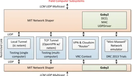
Figure 8: Detailed view of the networking components of the MIT DRC software system (full system in Fig. 6). To simulate network degradations that might occur between operators and robot in a disaster zone, various tools were used to artificially restrict throughput and increase latency. The IP tunnels shown on the left were developed by our team to perform full robot simulations before the contest tools were completed. To transfer data efficiently between the OCU and the robot, compression (source encoding) and queuing was performed by the network shaper. Packets were transmitted using UDP to avoid the often unnecessary overhead of TCP.
To address the throughput restrictions, we developed a tool called the network shaper that used source encoding, decimation, and priority queuing of messages destined to travel between the OCU and the robot. This tool relied on the Goby2 communications library, which was originally developed for very low-rate underwater acoustic data links (where average throughput is on the order of 100 bits per second), and was thus suitable for extension to this somewhat higher data-rate regime. Goby2 includes the Dynamic Compact Control Language (DCCL) which is an interface description language (IDL) coupled with a set of extensible source encoders for creating very small messages by taking into account the precise bounds of the data values to be transmitted in a given message’s fields. Goby2 is discussed in detail in another paper submitted to this special issue.1 The modest amount of added latency was ameliorated by the operator developing each plan
locally and transmitting it to the robot, which executed the plan autonomously as described in Section 4. Throughput and latency limits were implemented using a separate computer (the “Mini-Maxwell” developed by InterWorking Labs) with a network bridge running Linux and the network emulator (“netem”) traffic queuing discipline (“qdisc”) which can be manipulated (in testing) with a traffic control (“tc”) tool. The particular implementation used for the competition incorporated large buffers that held 10 seconds of data after the throughput limit was reached. Since this buffer length was 1-2 orders of magnitude greater than the latency introduced by the under-capacity link, timely operator response required ensuring that the throughput limit was never reached. Since the buffers were so large, it was not feasible to automatically detect available throughput by measuring packet loss, as the discovery time would be on the order of the network band alternation time. Thus, the network shaper autonomously detected the current band in use by measuring the latency of every packet and rate-limited all outgoing packets to avoid exceeding the Mini-Maxwell’s buffers.
This approach was effective until the latency/bandwidth settings were accidentally switched by the contest operators, such that the 1Mbps throughput regime was paired with 500ms latency setting and the 100Kbps
throughput paired with 50ms latency. During the 100Kbps band, data would fill the buffers of the Mini-Maxwell, leading to ten-second latencies at the OCU. To compensate during these runs (we were not aware of this inadvertent switch until the competition began), the operator was able to use the data request functionality in our interface to manually throttle downlink bandwidth and avoid saturating the buffers. This experience stresses the importance of properly designing the underlying network link between the OCU and robot, and has led us to believe that small buffers would be preferable for avoiding artificially high latencies and for rapid automatic detection of the network throughput. While the settings of the Mini-Maxwell were outside the control of our team for the competition, a real disaster-zone network could easily be designed to have modest buffers, as unlike latency and packet loss, buffering is a human addition to a network.
Figure 8 shows a diagram of the system components related to networking. For testing purposes, we developed our own restricted network tool (also based on “netem” over a layer 3 IP tunnel) that could allow single or multiple machine simulations of the entire operator/robot system.
3.4 System Management
In the VRC we utilized two robot-side computers (focused on control and perception respectively) and up to three base-side UIs, while in the DRC Trials our control and perception subsystems ran on a single robot-side computer.
To manage this distributed computing architecture we utilized another tool developed during the DUC called procman (Leonard et al., 2008). Via a simple user interface, called procman sheriff, operators could launch our system on each of the host machines (called deputies) with a single mouse click, monitor memory usage and process behavior, and manage computation load. Procman also allowed us to easily keep track of the robot model configurations we used in different tasks.
Because of the restricted communication channel, we modified procman to ensure that no recurring band-width usage occurred: a summary of the system status was delivered only upon a detected change, rather than continuously, and process names were hashed rather than being sent in plain text.
4 Motion Planning
Our planning infrastructure enabled us to pose and solve a wide variety of motion planning problems. The two key components of our approach were an efficient, optimization-based inverse kinematics (IK) engine and an automated footstep planner. The former allowed us to describe the requirements for a given motion in terms of a library of kinematic constraints. Our IK engine translated these constraints into a nonlinear program that was then solved to yield a feasible motion plan. The footstep planner converted user-specified navigation goals into a sequence of footsteps that respected constraints on the relative placement of successive footsteps. This section describes the capabilities of these planners, which provided the language into which our user interface translated the user’s intent.
4.1 Efficient inverse kinematics engine
Our specification for a kinematic motion planner required that it be efficient, i.e. capable of producing feasible whole-body plans for Atlas in much less than a second, and expressive, i.e. capable of reasoning about a variety of constraints and goals. Although efficient Jacobian-based algorithms for computing local IK solutions exist (e.g., (Buss, 2004)), they cannot easily incorporate arbitrary objectives and constraints. Therefore, we cast IK as a nonlinear optimization problem that we solved locally using an efficient implementation of sequential quadratic programming (SQP). Results generated by the IK engine were of one of two types: 1) a single robot configuration, or 2) a smooth time-indexed trajectory of configurations.
Single-shot IK: For a single configuration problem, the objective was to minimize the weighted L2distance
from a nominal configuration,
arg min q∈Rn (qnom− q) TW (q nom− q), subject to fi(q) ≤ bi, i = 1, . . . , m,
where qnom∈ Rn is a nominal configuration of the robot in generalized coordinates (for Atlas, n = 34), and
fi(q) : Rn → R, i = 1, . . . , m is a set of kinematic constraint functions. This type of optimization can be
used to, e.g., find a configuration for reaching to some target position while remaining as close as possible to the current standing posture.
Trajectory optimization: For many problems of interest, finding a single configuration is not sufficient. Rather we would like the robot to achieve a complete motion that is smooth and respects some set of (possibly time-varying) constraints. To generate configuration trajectories in this way, we formulated an optimization problem over a finite set of configurations, or knot points, interpolated with a cubic spline. The trajectory optimization problem had the form
arg min q1,...,qk k X j=1 (qnom,j− qj)TW (qnom,j− qj) + ˙qjTWv˙qj+ ¨qTjWa¨qj, subject to fi(q1, . . . , qk) ≤ bi, i = 1, . . . , m,
where additional costs associated with the generalized accelerations and velocities at each knot point were added to promote smooth trajectories.
The API to the IK solver allowed the user to specify a variety of constraints to flexibly generate whole-body configurations and trajectories. The supported constraint types included:
• joint limits
• pose of end-effector in world/robot frame (bilateral and unilateral) • cone (gaze) constraints of end-effector in world/robot frame • distance between two bodies
• center of mass position and quasi-static constraints • linear configuration equalities (e.g., left/right symmetry)
Here “end-effector” should be interpreted to be any frame attached to a rigid body. For trajectory optimiza-tion, it was also possible to specify time windows during which subsets of constraints were active.
IK problems were solved using an efficient SQP implementation that exploits structure shared between most problem instances. Due to the tree-structure of the robot’s kinematics, the constraint gradients are often sparse. For example, a constraint function on foot pose is unaffected by changes in the position of the torso DOFs. Using SNOPT (Gill et al., 2002), we were able to solve single-shot IK problems in approximately 10ms and find smooth motion trajectories with 5 knot points in 0.1s to 0.2s. As discussed in Section 7.1, this was essential to enable online planning of entire motions.
On occasion, the solver was not able to find feasible points. When this happened, the user was notified and it was up to her to make adjustments to the constraints and resubmit the request to the planner. Optionally, the planner could successively relax constraints, such as end-effector pose, until a feasible plan was found. In this case, the feasible plan would be returned to the user along with information about the degree of relaxation.
4.2 Planner Classes
To promote faster and more predictable interaction between the operator and the IK engine, we developed several planning classes that employed canonical sets of constraints and objective functions. This allowed the operator to succinctly specify inputs to the planner through the user interface (Section 5) rather than having to completely construct planning problems before each action.
The manipulation planner responded to end-effector goals generated by the operator. The input could be of the form “reach to this hand pose,” which was converted to a position and orientation constraint on the active end-effector at the final time. In this case, the manipulation planner returned a time-indexed joint-angle trajectory from the robot’s current posture to one that satisfied those constraints. The operator could specify the behavior of the rest of the body during the reach by selecting from two planner modes: one that kept all other end-effector poses fixed, and one that allowed whole-body motion.
It was also possible to input a trajectory of end-effector goals to generate a manipulation plan. For example, as illustrated in Section 5.2.2, the operator could request a valve turning plan by simply rotating a valve affordance with a grasped hand attached, hence defining a desired end-effectory trajectory.
The end-pose planner responded to operator requests for a feasible configuration from which to perform a manipulation. Given a time-indexed set of end-effector goals, the end-pose planner used the IK engine to simultaneously search for a smooth manipulation trajectory and a feasible constant standing posture from which the manipulation could be executed. This posture could then be used in turn to generate appropriate walking goals so that desired manipulation could be carried out after the robot finished walking to the object of interest.
The whole-body planner responded to inputs containing desired footstep locations, a set of end-effectors to keep fixed, and high-level motion parameters such as desired foot clearance over the terrain map or bounds on pelvis sway. This planner generated smooth, whole-body configuration trajectories that satisfied the foot and end-effector pose constraints in addition to quasi-static constraints that kept the robot’s center of mass ground projection within the support polygon of the feet. This planner was used in the trials to climb the ladder.
Finally, the posture planner was the simplest planner. Its input was a desired joint configuration for the robot, for which it would return a smooth trajectory from the current configuration to the goal. This planner was useful for moving to a pre-scripted joint configuration that, e.g., retracted the right arm close to the body to move through a tight space.
4.3 Footstep Planning
Somewhat separate from the IK-based planners, the footstep planner was used to determine automatic footstep placement given a high-level goal from the human operator, as well as detailed input from the user about the specific location of a particular footstep if required. Specifically, given the robot’s current configuration and a desired goal pose expressed as a position and orientation on the surface of the perceived terrain, the footstep planner computed a sequence of kinematically-reachable and safe step locations to bring the robot’s final standing position as close as possible to the goal, while allowing easy operator adjustment of the plan. The planner minimized the total number of steps required to reach the goal by exhaustively searching over all numbers of steps between a user-specified minimum and maximum, typically one and ten respectively, and choosing the plan with the fewest steps which still reached the goal (or the plan which came the closest to the goal if none could reach it). Each search for a plan with a fixed number of steps required approximately 10 ms, so exhaustive enumeration over a variety of numbers of steps was not prohibitive. Kinematic reachability of a footstep plan was ensured by constraining the location of each step to within a polyhedron defined relative to the pose of the prior step. This reachable polyhedron was computed offline by
min. width nominal width max. width forward step backward step x y min. width nominal width max. width forward step backward step x y
Figure 9: Left: A simplified representation of the kinematic reachability region for footstep placement. Given a fixed position and orientation of the right foot, we compute a polyhedral region defined by parameters min width, max width, etc. into which the next position of the left foot must be contained. In practice, this polyhedron is represented in four dimensions: x, y, z, and yaw, but only x and y are drawn here. Center: several example locations for the left foot (red) relative to the right foot (green). Right: A complete footstep plan from the robot’s position to the target position and orientation showed by the green circular marker. In this particular plan, the robot steps forward, then to the side, then backwards in order to reach the goal.
fixing the position of one foot and running inverse kinematics on a wide range of possible positions for the other foot. The step locations for which the inverse kinematics problem was feasible were then converted to a polyhedral inner approximation, which provided a conservative, convex set of locations for the placement of one foot relative to the prior step location. A simplified cartoon of this polyhedral approximation is shown in Figure 9. The primary planning algorithm used during the DRC was a simultaneous nonlinear optimization of the position and orientations of several steps, typically one to ten. The optimization attempted to minimize the error between the final steps and the goal, while respecting the polyhedral reachable regions. This approach differs from the footstep planning methods used by Huang (Huang et al., 2013), Chestnutt (Chestnutt et al., 2003), and Kuffner (Kuffner et al., 2001) in that it performs a continuous optimization over the positions of the footsteps, rather than reducing the choice of step location to a discrete selection among a few pre-computed relative step positions.
Once the planner had generated a candidate footstep plan, it was presented to the operator as a sequence of footsteps, as shown in Figure 9. The x and y positions and yaw of each step could be individually adjusted through the user interface, and the planner ensured that the roll, pitch, and height of each step matched the estimated terrain underfoot. The height map representation used in planning performed a RANSAC plane fit to fill in the gaps in the as sensed height map. Since the lidar provided no data about the ground near or under the robot’s feet, the height map used the forward kinematics of the robot’s legs to find the height and orientation of the bottoms of the feet to estimate the terrain directly underfoot and within a 1 meter square region around the robot.
During the VRC, we used an edge detection filter to classify areas of the terrain that were too steep or rough to step on, and the footstep planner was constrained to avoid placing steps on these regions. However, the generally flat terrain of the DRC made this approach less useful, and the extremely precise footstep positioning during the rough terrain task was primarily done manually, so this capability was not used during the DRC trials.
5 User Interface
The rich motion planning system discussed in the previous section enabled us to design a robot interaction system at a higher level than traditional low-level teleoperation. Specifically we sought to interact with the world at the level of affordances. We defined affordances as objects of interest that could be physically acted upon by the robot to perform some task-specific goal. These objects were specified as a series of links and joints organized in a tree structure similar to the well-known Unified Robotic Description Format (URDF) used to represent the kinematic structure of robots (Sucan, 2014). We extended this format to enable templatization and termed it the Object Template Description Format (OTDF). Figure 10 shows some example affordances which were described by OTDF.
The primary robot operator could manually specify the parameters of these objects, or could instead draw upon the output of a semi-automated lidar fitting system (controlled by the perception operator) which detected and positioned objects relative to the robot in our 3D interface.
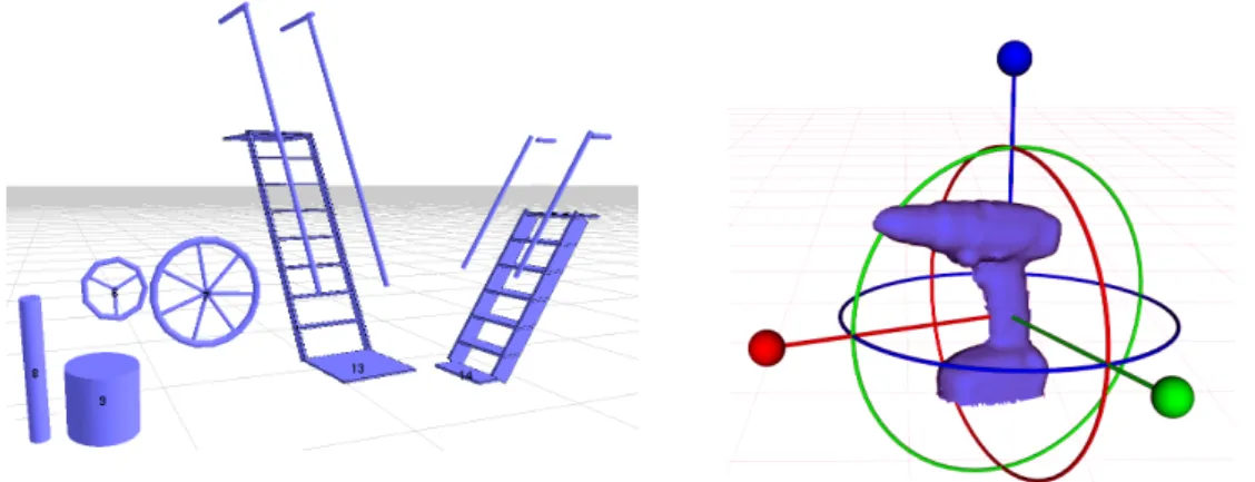
Figure 10: Affordances were represented via a parameterized XML format. Left: a collection of objects under three templates: i) cylinder; ii) valve; and iii) angled-ladder. Two pairs of objects are shown under each affordance class, which are instantiations with different parameters. Right: Interactive markers allowed the user to adjust the position of an affordance, or to instruct the robot to move the affordance along one of its internal degree of freedom.
5.1 Affordance fitting
We developed both automatic and human assisted object fitting algorithms for the competition. While we had some success with fully automated fitting, we focused more on human assisted fitting due to the competition rules. In the DRC Trials, unlike the VRC, operator input (OCU-to-robot bandwidth usage) was not penalized, and the extra time required to provide human input to a fitting algorithm was small compared with the time lost due to planning robot motion with a poorly fit affordance model. Thus, human assisted fitting algorithms were used in all five of the DRC Trials manipulation tasks.
The operator provided input by specifying initial search regions, and by accepting or adjusting pose esti-mation post-fit. Search regions were input either by 3D point selection in the lidar point cloud or by 2D annotations on point cloud projections or renderings. Images from all onboard cameras were fused and could be viewed interactively for visual context (Figure 12).
One human assisted algorithm was developed for the debris task to enable rapid fitting of lumber of arbitrary dimensions laying in unstructured configurations with overlap and occlusions. The algorithm was designed to fit rectangular prisms, and could be applied to boards, cinder blocks, bricks, and boxes. The operator began by selecting the expected cross-sectional dimensions of the affordance; for instance, lumber cross sections are typically 2×4 in, 4×4 in, or 2×6 in.
Figure 11: A fitting algorithm produces an affordance that can be used to plan a reach motion. Left: A line annotation defines a search region that is used by a segmentation algorithm to fit a 2”x4” board affordance to the 3D point cloud data. Right: An end-effector goal placed on the board affordance is used to compute a reaching plan.
Figure 12: Left: an example of foveation during the debris task to enhance the operator’s situational awareness without drastically impacting bandwidth. The operator selects a region of interest on a low-resolution image to request a high-low-resolution sub-image. Right: a first-person combined view stitches the head camera image with the left and right fisheye chest camera images. The operator can use the mouse to zoom and look in all directions for superior situational awareness.
The operator then defined the search region by drawing a line annotation on the display using mouse clicks to define the endpoints. This annotation could be drawn either on a camera image or a 3D point cloud rendering; in practice we always annotated using the 3D rendering because the camera’s limited field of view did not always cover the region of interest. The line end points were projected as rays in 3D originating from the camera center to define a bounded plane, and points in the lidar point cloud within a threshold distance of this plane were kept as the initial search region.
Given the initial search region, the board fitting algorithm used RANSAC with a plane model to select inlier points that were then labeled as board face points. These were binned along the vector parallel to the edge connecting the search region ray end points, which was roughly parallel to the board’s length axis. The algorithm identified one candidate edge point in each bin by selecting the maximum distance among that bin’s points along the vector perpendicular to the ransac plane normal and length axis. Due to occlusions and adjacent surfaces, not all candidate edge points were true board edge points, so a RANSAC line fit was applied to the candidate edge points to label inliers presumed to be the board edge. The board affordance model was snapped to the fitted face plane and edge line, and stretched along the edge line to encompass the minimum and maximum face point projections onto that line.
affordance server which maintained the states of all identified affordances in the vicinity of the robot and made them available to both the user interface and the planners. Combined with the current robot state, this information provided inputs necessary for the operator to plan action sequences.
5.2 Primary User Interface
Figure 13 shows a screen capture of our primary user interface. Within this viewport the operator perceived the robot’s vicinity, queried planners, reviewed plans, and monitored plan execution. A robot avatar, the current affordances, and views of the lidar data were rendered in 3D in the main viewing pane. From the side panels, the user could interact with plans, request new sensor data, and change data visualization properties.
Figure 13: The primary user interface showing the 3D robot avatar while the operator planned a pre-grasp reach to a hose. The candidate motion plan contains modifiable key frames in red, yellow and teal (Section 5.2.2). A grasp goal or sticky hand (green) is fixed to an (obscured) model of the hose. Also visible are controls for executing the plan, making perception data requests immediately or at a specified streaming frequency, and adjusting image quality and workspace viewport. 3D data views could be toggled, resized or color mapped (in this case by height).
5.2.1 Interaction with Affordances
The operator interacted with affordances primarily to specify inputs to the task planners. A double-click would launch a user menu that was unique to each object instance. The menu enabled the operator to perform tasks such as adjusting the pose of the object; adjusting the internal state of the object (e.g. joint DOF positions); seeding grasps, footsteps or gaze goals; searching for robot postures to achieve these goals; and finally loading corresponding goal seeds from storage. Interactive markers (shown in Figure 10 for a drill) could be used to adjust the pose of the object and its internal state. We also developed a 3D mouse interface for some of these tasks, but our experiments with it did not demonstrate a significant advantage over the combination of a traditional mouse and keyboard.
Left: Joint-level teleoperation. Right: Prior posture configuration.
Left: End-effector goal specifying a 6-DOF pose constraint. Right: Gaze goal specifying an orientation constraint.
Left: Sequence of poses to generate motion path. Right: Navigation goal specifing destination pose.
Figure 14: Our interface supported a variety of user specified goals. Here a number of modes are illustrated with increasing complexity.
and 14). In the case of grasping, the user could query an optimizer by selecting the position on the object where s/he wished the robot to grasp. The optimizer solved for a feasible grasp that satisfied force closure constraints. Alternatively, the user could take advantage of pre-specified canonical grasps for known objects; for example, after fitting a door frame, the operator would immediately be presented with the location of a pre-grasp hand position relative to the door handle.
These phantom end-effector seeds, termed sticky-hands and sticky-feet, provided a mechanism to transform affordance-frame commands into end-effector commands which are more easily handled by the robot-centric planning and control modules. The seeds could be committed to planners as equality constraints (or desired goals) or as desired posture set-points for grasp control.
5.2.2 Interactive Planning
The user interface permitted bidirectional interaction between the operator and planners. An important consequence of this interaction was that input from the operator could be used to guide the planner away
from undesirable local solutions by refining a proposed plan with additional constraints. A key feature that enabled this bidirectional interaction was key frame adjustment, which provided a mechanism for performing re-planning interactively.
Key frames were samples from a proposed robot plan that could be interacted with. Examples are illustrated in red, yellow and teal in Figure 13. By modifing the key frame’s end-effector location, position constraints could be added to the planning problem, allowing the operator to, for example, guide the optimization algorithm to plan motions around workspace obstacles.
5.2.3 Additional Components
The UI also provided simple controls to manage and visualize data provided by the Perception Data Server described in Section 3.2.3. Figure 13 depicts relevant UI panes responsible for server data selection (which particular camera images and 3D data view presets to request). The user could also customize the display of 3D data received from the robot, controlling visual representation (e.g., point cloud, wireframe, or mesh) and 3D color coding (e.g., texture map from the cameras or pseudo-color by height or by range); we typically used point clouds and wireframes with height-based color mapping. Control of sensor settings (including camera frame rate, gain control, and lidar spin rate), compression macros (“low”, “medium”, or “high” quality) was also available.
A secondary graphical user interface was used primarily by a human co-pilot for object refitting and pre-senting alternative views, such as the stitched camera view shown in Figure 12. Finally, a simple keyboard interface was used to make minor but precise adjustments to the end-effector position and orientation in several tasks.
6 Plan Execution
Operator-approved plans were carried out by streaming references from the field computer to controllers executing on the robot. By combining low-level position control with feedback from the arm joint encoders, we achieved sub-centimeter end-effector position error. For each joint, the hydraulic valve input current, c ∈ [−10, 10] mA, was computed by a simple PID rule:
c = Kp(qref − q) + Kd( ˙qdes− ˙q) (2)
qref = qdes+ Ki
Z t
0 (qdes− qenc)dτ, (3)
where q and ˙q are the filtered joint position and velocity signals computed from the actuator LVDTs, and qenc is the joint encoder measurement. Due to API restrictions, the robot servo loop signals were limited
to LVDT-based joint positions and velocity estimates, so the PD rule (2) was executed onboard the robot at 1000Hz, while the references (3) were computed at 333Hz and streamed to the robot from the field computer. Due to significant velocity noise in the unfiltered ˙q signal (some arm joints had noise standard deviations greater than 3 rad/s), we used aggressive 5Hz 1st order low-pass filters to prevent undesirable high-frequency effects in the control loop. The time-varying desired joint positions and velocities, qdes and
˙qdes, were evaluated directly from the smooth joint trajectories generated by the planner.
We exploited the robot’s available balancing and stepping behaviors to produce manipulation and walking motions. Coordinated upper-body and pelvis motions were achieved by streaming pelvis pose references to the balancing controller. Likewise, footstep plans were used to generate appropriate references for the stepping controller. For ladder climbing, position control of the entire body was used to follow whole-body, quasi-static climbing trajectories. A primary focus of our DRC Finals effort is replacing these behaviors with a custom whole-body, dynamic controller for manipulation and locomotion that will increase execution speed, stability, and reactivity. More details about this control approach are described in Section 8.3.
7 DRC Trials
We fielded our system in the DRC Trials held at Homestead Speedway in Miami, Florida on December 20-21, 2013, which represented the largest ever demonstration of robot multi-task capability in an outdoor environment and were far removed from laboratory conditions. The Trials served as an intermediate progress evaluation and funding down-select before the DRC Finals expected to take place 12-18 months later. We competed against 6 other teams using a Boston Dynamics Atlas, and 9 teams who built or brought their own robots. We finished in fourth place with 16 points – behind Schaft of Japan (27 points), the Florida Institute for Human and Machine Cognition (IHMC) (20 points), and CMU’s CHIMP robot (18 points). IHMC used an Atlas robot.
The following table summarizes the outcome of the eight tasks in the order in which we attempted them. Teams had 30 minutes to complete each task. One point was scored for completion of each of three ordered subtasks; completing all three subtasks without intervention earned a bonus point. Interventions could be called by the robot operator or by a member of the field team, triggering a minimum 5-minute penalty period during which teams could reset their robots behind a checkpoint. We attempted all eight tasks and scored in all but one (driving), achieving the maximum four points in the drilling and valve tasks.
Task Score Objective Summary Debris 1 pt Clear 10 pieces of wood,
walk through corridor Cleared 5 pieces of wood, recovered from dropping twonear robot’s feet Hose 2 pts Grasp and mate hose with
a standpipe Grasped hose, failed to mate hose with standpipe Valves 4 pts Turn one lever valve and
two wheel valves Succeeded without intervention, despite erroneous net-work behavior Drill 4 pts Grasp and turn on a drill,
cut triangle pattern in wall Succeeded without intervention, see Section 7.1 Door 1 pt Open and walk through
three doors Opened and walked through one door, fell over unex-pectedly Vehicle 0 pts Drive a utility vehicle
through course, exit vehicle Drove approximately half the course before time expired Terrain 3 pts Walk across increasingly
difficult terrain Succeeded after an intervention, one of three teams tofinish Ladder 1 pt Climb a 10-foot ladder at a
60-degree incline Climbed to second step, fell sideways against railing To give the reader a better understanding of the operation of the robot through our system, we provide a detailed account of our drill task execution at the Trials in the next section. To summarize the remainder of our Trials experience, we highlight a few noteworthy observations and issues that occurred:
• In the debris task, a mistake while dropping two debris pieces required our operators to adjust their high-level task sequence and pick up a piece of wood at the boundary of kinematic reachability and sensor visibility. This effort allowed us to score a point in the last remaining seconds, and was a strong, albeit stressful, demonstration of our system’s ability to plan and execute motions in unanticipated situations.
• In the hose and valve tasks, a misconfiguration in the competition network resulted in long commu-nications blackouts. For example, after confirming a footstep plan to approach the hose, we did not receive a sensor update from the robot until it was standing in front of the hose. We were pleased that our system and operators could deal gracefully with this unexpected situation, with the sole side effect being slower task execution.
• As with other teams, wind was an issue for us. In the door task, our operator innovated a two handed strategy to push open the first door, constantly applying pressure against it to prevent it
from blowing closed. In the terrain and climbing tasks, we repeatedly had issues with the wind interfering with robot IMU initialization.
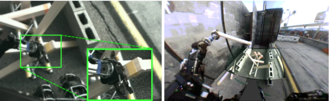
• As illustrated in Figure 15, lighting conditions were very challenging. Strong shadows made even human-aided perception difficult. We had anticipated this and therefore relied heavily on lidar-based perception with no automated vision algorithms. Nonetheless, with low-rate (∼1Hz) lidar updates this approach has limited capacity to support fluid, closed-loop control and perception.
• In the climbing task we used steel hooks instead of actuated hands to brace the robot’s considerable mass while ascending the ladder. Similarly, using simple unactuated metal pointers offered the most robust solution for opening doors, pressing buttons, and turning valves. The fact that nearly every Atlas team adopted similar appendages for these tasks suggests that dexterous hands capable of greater strength and stiffness might significantly improve the versatility of disaster robots.
7.1 Wall Drilling Task
We will focus our detailed discussions on the drilling task, which exercised most of our system’s compo-nents and required a full range of planning—from low-level end-effector adjustment to more sophisticated constrained motion plans. The drilling task involved walking to a table, picking up a drill, turning it on, walking to a dry-board wall, cutting out a triangular section of the wall, and pushing the cutout free of the wall. The threshold for scoring any points was relatively high; each of the first two points was awarded for cutting one line segment of the triangle and the third point required cutting the third segment and success-fully knocking the triangle loose. Any cuts into the wall too far away from the triangle edges immediately voided that edge and eliminated the possibility of the third and fourth points. This resulted in most teams operating quite slowly and carefully.
Charts detailing task execution during the DRC Trials are illustrated in Figure 16, whose first row illustrates progress through the task over time. The initial phase of the task went smoothly and, after 3 minutes, the robot had reached for the drill and was ready to grasp. Reaching consisted of a scripted posture that raised the hand up and around the table, followed by a single reaching plan directly to a sticky hand attached to a model of the drill that had been fit by the perception operator. However, after reaching to the pre-grasp position, the operator realized that the hand was unresponsive and would not close around the drill. During a three-minute delay we quickly resolved the issue and grasped the drill. We learned after the event that the problem was due to wiring damage that caused intermittent electrical connectivity to the hand.
After grasping the drill, the operator commanded the robot to lower its arm and step to the side of the table. In our experiences in the lab walking with the drill and firehose in hand, we found that holding masses close to the torso gave improved stability. After walking up to the wall, the operators raised the drill into the head camera view using the posture planner, and re-fit the drill affordance precisely relative to the hand using the 3D fitting interface. From this point forward, the drill affordance was assumed to be fixed to the hand frame and all drilling motions would be executed relative to the drill-bit frame. A plan was then generated to re-position the drill so that 1) the power button would be clearly in view of the camera and 2) the button would be reachable by the right hand.
Using the pointer on the right hand and end-effector teleoperation relative to the camera frame, the operator pressed the drill’s power button. While this motion could easily be expressed by our affordance-based plan-ning system, the combined imprecision of the forward kinematics and perception data made sub-centimeter autonomous motions unreliable. During practice sessions, we verified that the drill had been turned on using audio continuously streamed across the network link from the onboard microphone. However, in the competition, background noise from the wind and crowd made it impossible to discern the sound of the drill motor. After realizing this, the operators captured a high-resolution image chip of the drill button to determine that the drill was on.
Figure 15: Top left: head camera view of poker used to press drill’s power button. Top right: visualization of the nominal plan to reach all drill target points in the triangle. Bottom right: head camera view provides situational awareness to operator as robot executes drilling plan. Bottom left: Robot avatar and RGB point cloud visualization with affordance models of the drill and triangle target.
aligned to the RGB-colorized lidar view. After the operator clicked on each triangle vertex in the image, the system intersected the corresponding back-projected view rays with a wall plane that was automatically fit to the lidar data.
7.1.1 Drilling: Multistep Plan Generation and Validation
Executing the drilling motion (in a single sequence) was one of the more complicated planning capabilities we fielded in the Trials. For complex, multi-step manipulation tasks such as this, a greedy approach to plan generation has the possibility of failing mid-sequence, leaving the robot stuck in a state where the next step is kinematically infeasible. To address this issue, the planner attempted to ensure task feasibility when given a full task description (in this case the geometry of the triangle). First, before the robot even approached the wall, all kinematic constraints from the task were sent to the planner to generate a comprehensive motion. Such a plan is visualized in Figure 15. Included in the generated plan was an appropriate place to stand at the wall, which the planner then synthesized into a goal for the walking planner.
Once the robot reached the wall, the planner was queried again to generate a complete cutting motion that kept the tool axis perpendicular to the wall and at a constant depth inside the wall, and for which the robot would remain quasi-statically stable. Like the previous multi-step plan used to generate a walking goal, this motion was not executed as a single plan. However, its existence ensured feasibility of the entire motion, and it was used as a seed to generate the subsequent smaller plans in the sequence.
7.1.2 Supervised Autonomous Plan Generation
The structure of the remainder of the task lent itself to a straightforward se-quence:
1: Move drill in front of first target, avoiding collisions with the wall. 2: Drill into first target
3: for Each line segment to cut do 4: while Line segment is incomplete do 5: Cut along line segment
6: Refit triangular affordance 7: end while
8: end for
Each robot motion above required approval by the operator. The planner automatically corrected for devi-ations from the desired path, and transitioned to the next line segment when it judged the cut to be within the target region. Ultimately, however, the user supervised these autonomous plans and could, at any time, instead generate a teleoperated cutting motion on the plane of the wall.
A challenge while cutting the wall was maintaining an accurate state estimate in the presence of significant external forces and joint backlash. This uncertainty made shorter motions advantageous, since they mini-mized the risk of cutting outside the allowable regions. Manual refinements to the position of the triangle affordance (adjusted by sliding in the wall plane) also helped, and demonstrated a tight loop between (hu-man) perception and robot control. The degree of autonomy embedded in the planner greatly increased speed of execution, while still allowing for relatively short, safe cuts.
At the 18th minute we commenced cutting and cut the entire pattern in a total of 8 minutes. After the edges were cut, we reverted to teleoperating the drill in the plane of the wall to push against the triangle, and finally, with a few minutes remaining, we dislodged it.
7.1.3 Analysis of Operation and Communication
As illustrated in Figure 16, we operated the robot in a variety of manners—from scripted sequences to operator-supervised autonomy. In total we executed 4 walking plans and 86 motion plans during the drill task. The vast majority of those were in semi-autonomous mode (salmon colored section), in end-effector teleoperation mode (blue), and in affordance-relative reaching. We aim to improve upon this in the coming year by implementing compliant motion control (e.g., in the case of pressure against the wall). Also illustrated is time spent executing scripted motions (light green). Other significant time blocks included resolving the systems issue (tan), assessing the next action of a plan (purple), and manual affordance fitting (orange). The second plot in Figure 16 shows the percentage of time the robot was actively executing a plan, per 30-second period. Despite our operators’ complete focus on the tasks, the majority of time was spent stationary, with the robot moving only 26% of the time (35% if walking is included). While more fluid user interfaces would likely increase these numbers, we believe significant gains can be achieved by building more autonomy into our system.
The lower plot in Figure 16 represents bidirectional bandwidth usage for the task. We can see that the usage was heavily one-sided with incoming data from the robot (blue) outweighing plans communicated to the robot (red) by over two orders of magnitude. While not shown here, the configuration of the robot and its onboard sensors plus our own diagnostic information represented only 5% of incoming data—with the remainder being split between imagery and lidar. Note that the ripples in the data rate sent from the robot correspond to the 100kbps/1Mbps regimes alternating each minute.
These plots have several implications in the context of the networking parameters defined by DARPA that were intended to encourage autonomy. Firstly, imposition of the 100kps/1Mbps regimes required that each team implement downstream sensor data compression algorithms, but did not encourage autonomy as teams were free to transmit any number of commands upstream to the robot, provided the commands were suffi-ciently compact. Secondly, we found that the variable 50ms/500ms latency added in each of the alternating regimes had little effect on our operators’ actions, which typically proceeded in the following sequence: perceive relevant features, create a motion plan, transmit the plan, then monitor execution while data is returned. The time taken to transmit any plan to the robot was dwarfed by the other actions—in particular time spent by the human perceiving the surround and specifying and reviewing plans.
In summary, the bandwidth and latency fluctuations had little effect on our operation strategy. We also surmise that further reduction of the bandwidth (if applied uniformly) would not bring about an expected increase in autonomy—it would simply limit the operator to a sparser perception of the scene. Finally, it is our opinion that direct teleoperation, if implemented correctly, can be executed with much lower bandwidth requirements than our implemented semi-autonomous system. For these reasons we believe that autonomy would be more effectively incentivized through significantly larger latencies—on the order of 3–10 seconds— and by limiting the number of discrete commands that the operator can send to the robot.
8 Discussion
8.1 Limitations and Lessons Learned
From our experience thus far we have learned lessons along a number of dimensions: about the precision and accuracy with which we can control Atlas; about the viability of our high-level approach; about the operator burden implied by our approach; about the importance of planning for future (not just imminent) actions; and about our team organization.
When we formulated our high-level approach in early 2012, we anticipated being able to achieve reasonable kinematic precision and accuracy, i.e. that configuration space position tracking would yield accurate task