BayesDB : querying the probable implications of tabular data

BayesDB: Querying the Probable Implications of Tabular Data

by

Jay Baxter

Submitted to the Department of Electrical Engineering and Computer Science

in partial fulfillment of the requirements for the degree of

Master of Engineering in Electrical Engineering and Computer Science

at the MASSACHUSETTS WN81TtfE,

OF

MASSACHUSETTS INSTITUTE OF TECHNOLOGY

_JUL

₁₅

₂₀₁₄

June 2014

LIBRARIES

®

Massachusetts Institute of Technology 2014. All rights reserv .t-

-Signature redacted

Author ...

Departm't of/lectrical Engineering and Computer Science

May 23, 2014

Signature redacted

C ertified by ...

...

Vikash lnaninghfa

Research Scientist

Thesis Supervisor

/7 ..

Signature redacted

A ccepted by ...

_...

Prof. Albert R. Meyer

BayesDB: Querying the Probable Implications of Tabular Data

by

Jay Baxter

Submitted to the Department of Electrical Engineering and Computer Science on May 23, 2014, in partial fulfillment of the

requirements for the degree of

Master of Engineering in Electrical Engineering and Computer Science

Abstract

BayesDB, a Bayesian database table, lets users query the probable implications of their tabular data as easily as an SQL database lets them query the data itself. Using the built-in Bayesian Query Language (BQL), users with little statistics knowledge can solve basic data science problems, such as detecting predictive relationships between variables, inferring missing values, simulating probable observations, and identifying statistically similar database entries. BayesDB is suitable for analyzing complex, heterogeneous data tables with no preprocessing or parameter adjustment required. This generality rests on the model independence provided by BQL, analogous to the physical data independence provided by the relational model. SQL enables data filtering and aggregation tasks to be described independently of the physical layout of data in memory and on disk. Non-experts rely on generic indexing strategies for good-enough performance, while experts customize schemas and indices for performance-sensitive applications. Analogously, BQL enables analysis tasks to be described independently of the models used to solve them. Non-statisticians can rely on a general-purpose modeling method called CrossCat to build models that are good enough for a broad class of applications, while experts can customize the schemas and models when needed. This thesis defines BQL, describes an implementation of BayesDB, quantitatively characterizes its scalability and performance, and illustrates its efficacy on real-world data analysis problems in the areas of healthcare economics, statistical survey data analysis, web analytics, and predictive policing.

Thesis Supervisor: Vikash Mansinghka Title: Research Scientist

Acknowledgments

This thesis is based on collaborative research with Vikash Mansinghka, Dan Lovell, Baxter Eaves, and Patrick Shafto. I owe a great deal of thanks to all of them: my thesis advisor, Vikash Mansinghka, who has provided countless helpful insights and tips along the way, Dan Lovell for his work as lead developer on the CrossCat backend, Baxter Eaves for running experiments and working on the CrossCat backend, and Patrick Shafto for his general help, especially with usability design as BayesDB's first user. I would also like to thank Seth Berg, Mason DeCamillis, and Ben Mayne for helping out by using BayesDB to analyze real datasets and adding features to the codebase. Additionally, thanks to Tejas Kulkarni and Ardavan Saeedi for many helpful conversations about BayesDB, and my other friends and family for always being so supportive of me. And finally, thank you to the DARPA XDATA and PPAML programs and Google for sponsoring BayesDB development and my research assistantships.

Contents

1 Introduction

1.1 O verview . . . .

1.2 M otivation . . . .

1.3 Example data analysis . . . .

1.4 How does BayesDB work? . . . .

1.5 O utline . . . .

2 Bayesian Query Language (BQL)

2.1 Completing statistical tasks with BQL . . . . 2.1.1 Detect predictive relationships between variables and 2.1.2 Identify contextually similar database entries . . . . 2.1.3 _{Infer missing values with appropriate error bars . . .}

2.1.4 Generate hypothetical rows conditioned on arbitrary

quantify their strength . . . . .

predicates 2.2 Formal Language Description

2.2.1 2.2.2 2.2.3 2.2.4 2.2.5 2.2.6 2.2.7 2.2.8 2.3 Model Loading Data . . . . . Initializing Models and Btable Administration

Saving and Loading Bt Querying . . . . Query Modifiers . . . Column Lists . . . . . Predictive Functions Independence in BQL . . . . . . . . Running Analysis . . . . . . . .

ables and Models . . . .

. . . . . . . . . . . . . . . . . . . . 3 Implementing BQL

3.1 Interface between BQL and Models

17 17 18 20 25 25 27 27 27 . . . . 2 8 28 28 29 29 29 30 30 31 32 32 33 36 37 . . . . 37 . . . . . . . . . . . . . . . . . . . .

3.1.2 Prediction Interface . . . . 39

3.2 Implementation of Query Primitives . . . . 41

3.2.1 SIM ULATE . . . . . . .. . . 41

3.2.2 IN FER . . . . . . . . .. .. 41

3.2.3 WHERE clauses WITH CONFIDENCE . . . . 42

3.2.4 ESTIMATE COLUMNS . . . . 43

3.2.5 ESTIMATE PAIRW ISE . . . . 43

3.3 Functions . . . .. . . . . . . . . . . .. . . . .. 44 3.3.1 SIMILARITY . . . .. . . . . .. . . . . . 44 3.3.2 DEPENDENCE PROBABILITY ... ... 44 3.3.3 MUTUAL INFORMATION ... .... 44 3.3.4 TYPICALITY (row) ... .. ... 45 3.3.5 TYPICALITY (column) ... ... 45 3.3.6 PROBABILITY OF col=<val> ... 45 3.3.7 PREDICTIVE PROBABILITY ... ... 45

4 Indexer and Models 47 4.1 Model Descriptions ... ... 47

4.1.1 CrossCat, CRP Mixture, and Naive Bayes ... 47

4.1.2 Component Models and Data Types ... ... 49

4.1.3 Incorporating Prior Knowledge ... ... 49

4.1.4 Other Models ... ... 51

4.2 CrossCat's Implementation of BQL Interface ... ... 51

4.2.1 Inference Functions ... 52

4.2.2 Prediction Functions ... .. . ... 52

5 System Design and Architecture 55 5.1 C lient . . . .. . . . . .. . . . . 55

5.2 Parser ... ... ... .. ... ... ... . . . . ... ... . . 56

5.3 Engine . . . .. . . .. .. . . . .. . .. . . .. . . . 57

5.3.1 Data and Metadata . . . .. . .. . . . . . .. . 57

5.3.2 Query Processing Pipeline ... ... 61

5.3.3 Reliable Distributed Indexing and Model Balancing ... 62

5.4 Inference and Prediction Servers . . . . 62

38 3.1.1 Indexing Interface

6 Experiments and Quality Tests

6.1 _{BayesDB's query results are trustworthy in many cases . . . .}

6.1.1 _{Limitations of CrossCat, the current BayesDB backend} 6.2 6.3 63 63 . . . . . 64 . . . . . 65 . . . . . 71 Convergence Assessment . . . Inference Performance . . . . 7 Case Studies

7.1 Web Server Log . . . .. . . . .

7.2 Illustrations on Real Data . . . .

7.2.1 General Social Survey . . . . .

7.2.2 Chicago Crime . . . .

7.2.3 Flights . . . ..

8 Related Work

8.1 Probabilistic Databases (PDBMSes)

8.2 Automated Machine Learning Systems

73 73 79 79 83 85 87 87 88 89 89 89 90 91 91 9 Conclusion 9.1 Future Work . . . .. 9.1.1 Software Engineering . . . . 9.1.2 Performance Engineering . . . . 9.1.3 Modeling Improvements . . . .

9.1.4 Data Analysis Applications . . . .

9.2 Contributions . . . . . . . . 91

. . . . . . . .

List of Figures

1-1 Evidence for an impending shortage of data scientists: Many analysts, including

McKinsey, predict that the demand for data scientists will continue to rise much more rapidly than the supply of data scientists. Therefore, there is likely to be a huge demand for tools

like BayesDB that enable non-experts to complete some data science tasks [39]. . . . . 18

1-2 Comparison of traditional data analysis workflows to the BayesDB workflow . . . 19

4-1 Latent Structure from [23], [32]: Naive Bayes (top), CRP Mixture (mid), CrossCat

(bottom). Naive Bayes treats all columns as independent, and all rows are from the same component model. CRP Mixture still treats all columns as independent, but rows come from

different underlying component models (categories). CrossCat groups columns into views

(groups of dependent columns), each of which has its own different underlying categorization. 48

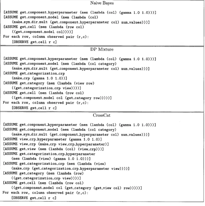
4-2 Venture code for Naive Bayes, DP Mixture, and CrossCat. A simple version of the

Naive Bayes, DP Mixture, and CrossCat models for multinomial data in Venture. Note that Naive Bayes has no views or categories, DP Mixture has categories, and CrossCat has both views and categories. Venture is a general purpose probabilistic programming language: for

details, see [22]. . . . . 50

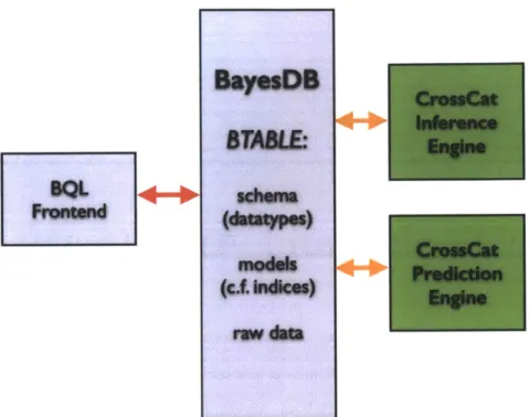
5-1 BayesDB System Architecture: BayesDB has four main components: the frontend (which

includes parser and client), the core BayesDB engine, an inference engine, and a prediction engine. The red arrow indicates a low-latency, low-volume connection, and the yellow arrows

indicate a high-volume connection. . . . . 56

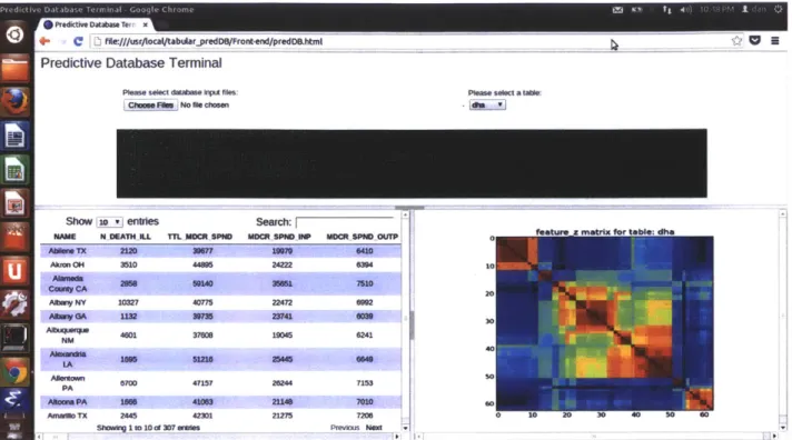
5-2 JavaScript Client: An initial prototype of what a web interface for BayesDB could look

like. The JavaScript client simply needs to implement the same functionality as the Python client currently does, but there is a possibility to convert the user's mouse clicks on the UI into BQL queries that are sent to the backend, thereby bypassing the need for the user to

6-1 An evaluation of BayesDB's ability to learn nonlinear relationships: The top row

of blue plots show four original datasets, which each have 500 points and have 0 correlation. However, by visual inspection, it is easy to see that there is a different nonlinear relationship that exists in each of these datasets. Traditional statistics typically uses correlation to quantify relationships between variables, but it has a critical flaw: it is only able to measure linear relationships. The bottom row of plots shows the relationship that BayesDB learns from each original dataset. In each case, the original data was loaded, 32 models were initialized and analyzed for 500 iterations, and we called SIMULATE 500 times to generate 500 new data

points from the joint probability distribution that BayesDB learned. . . . . 64

6-2 Testing BayesDB's ability to learn the full joint distribution: These plots compare

CrossCat with other simpler bayesian models (CRP mixture model and Naive Bayes, with hyperparameter inference for each model) on a synthetic 300x20 dataset generated by CrossCat with 4 views and 8 categories per view using 20 models with 500 iterations of MCMC for each. The top plot was generated by evaluating the probability of a held-out row using the BQL PROBABILITY function: it shows that the mean probability of a held-out row is lower for more complex models, as expected. CrossCat's hypothesis space is a superset of CRP mixture's hypothesis space, which is a superset of Naive Bayes' hypothesis space. The bottom plot shows that the mean squared error (MSE) of the predictive probability over each value in the

held-out row is lowest for CrossCat. . . . . 66

6-3 A comparison of missing value imputation accuracy between BayesDB and stan-dard and sophisticated baselines: In this experiment, we took a 250 row, 100 column

data table, removed a variable proportion of the data (x-axis): either 10%, 25%, 50%, 75%, or 90%, then loaded the data into BayesDB and generated 32 models with 300 iterations of analysis each, and used INFER to fill in all missing values with 500 samples from the posterior predictive for each missing value. CrossCat performs about as well as CRP Mixture at filling

6-4 An empirical assessment of BayesDB's calibration on synthetic datasets: These

experiments were run on a synthetic data table with 500 rows, 4 columns, 2 views, and 8 categories per view, where each category's data was generated from a multinomial distributed with 10 values. Afterwards, 20% of the data was randomly removed. The data was then loaded into BayesDB and analyzed with 32 models for 500 iterations. These three plots can be thought of as a multinomial P-P plot using normalized frequencies over missing values: each line represents the distribution of a column, where the y-axis is the inferred distribution and the x-axis is the actual distribution. These plots demonstrate that the three model types currently implemented in BayesDB (CrossCat, CRP mixture, and Naive Bayes) are all well

calibrated . . . . . 67

6-5 Experimental evidence that BayesDB's dependency detection is robust to the multiple comparisons problem: This experiment was run on a synthetic dataset with 100

rows and 32 or 64 columns, with two 2-column views. Therefore, the ground truth is that there are two pairs of columns that are dependent on each other, and all other pairs of columns are independent. This plot shows the dependence probability, as estimated by BayesDB using CrossCat, for all pairs of columns as a function of iterations. Each pair of columns is shown as a blue line, except for the two pairs of columns that are dependent according to ground truth. Before any iterations of inference, all pairs of columns start out with a fairly low yet uncertain dependence probability, accurately capturing BayesDB's uncertainty. After a number of iterations, the dependence probabilities have converged to their true values, showing

that BayesDB is able to discover individual relationships between variables in a robust way. 68

6-6 Empirical validation of CrossCat's MCMC sampler using the Geweke test: The

Geweke test is an inference diagnostic tool that compares the distributions of forward and backward sampled hyperparameters: in a correct sampler, the KL Divergence between those two distributions should converge to 0. The left plot shows a passing Geweke test, where all KL Divergences approach 0, and the right plot shows a failing Geweke test, where the KL Divergences do not all converge to 0 (this plot was used to diagnose a real bug in the sampler). 69

6-7 Estimates stabilize for DEPENDENCE PROBABILITY and INFER with more iterations: These plots show results on a real dataset: the Dartmouth Atlas of Healthcare,

with 20% of the data randomly removed. The error bars shown in the plots are standard errors calculated over 5 runs, where each run has 20 models and 100 iterations of MCMC. In the top plot, the two lines represent the dependence probability between two pairs of columns: as the number of iterations increases, the estimates stabilize, and the probabilities move from

50% towards their true value. The bottom plot shows the proportion of the missing data that

we are able to fill in with a confidence level of 10%: initially, only a small portion of the data is filled in, and the number of cells BayesDB is able to fill in at a given level of confidence

increases with the number of iterations. . . . . 70

6-8 Timing Plots: Inference time (time per step, the y-axis in these plots) increases linearly in

List of Tables

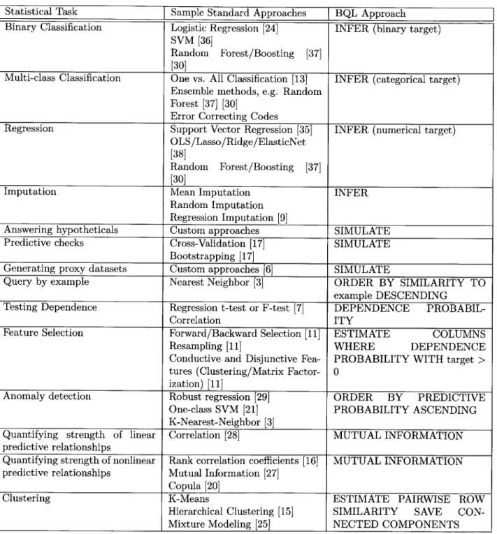
1.1 _{BQL queries corresponding to specific statistical tasks: For any given statistical task,}

there are often a huge number of models, techniques, and algorithms that could be appropriate to use. This is the issue that scikit-learn tries to solve with their cheat sheet (see Figure 1-2c). Instead of a cheat sheet or complex workflow, BQL queries specify the task that should be solved, and the implementation of how that task is performed is abstracted as a black box to

novice users (but is tunable/diagnosable for experts). . . . . 21

3.1 Which models implement which parts of the BQL Prediction Interface: This

ta-ble shows the parts of the BQL interface different model classes are capata-ble of implementing, including CrossCat, DPM (Dirichlet Process Mixture Model), NB (Naive Bayes), PGM (prob-abilistic graphical models), PGM+SL (prob(prob-abilistic graphical models with structure learning),

and KDE (kernel density estimation). . . . . 40

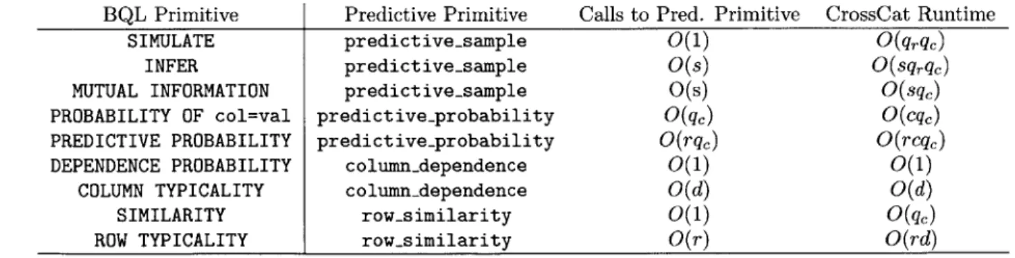
3.2 Implementation of BQL primitives: Each BQL query primitive is implemented using

only one function in the BQL prediction interface. This table can be used in conjunction with Table 3.1 to determine which BQL queries are possible with each type of backend. In addition, the runtimes for BQL Primitives are given both in terms of number of calls to the predictive primitive (the functions in the prediction interface) and the overall runtime with the predictive primitive implemented by CrossCat (where predictive..sample runs in 0(1) for imputation

and O(qc) for prediction, predictive-probability runs in

O(c),

in 0(1), and row-similarity runs in O(qc), as shown in Section 4.2.2). Let s indicate the number of predictive samples parameter. Let q, indicate the number of queried columns and let q, indicate the number of queried rows (e.g. specified by a parameter in SIMULATE, or

by the number of rows that matches the where clause in INFER). c indicates the maximum

number of categories over all

e

E.

Chapter 1

Introduction

1.1

Overview

BayesDB, a Bayesian database table, lets users query the probable implications of their tabular data as easily as an SQL database lets them query the data itself. Using the built-in Bayesian Query Language

(BQL), users without statistics expertise can solve basic data science problems, such as detecting predictive

relationships between variables, inferring missing values, simulating probable observations, and identifying statistically similar database entries.

BayesDB is suitable for analyzing complex, heterogeneous data tables with up to tens of thousands of rows and hundreds of variables. No preprocessing or parameter adjustment is required, though experts can override BayesDB's default assumptions when appropriate.

BayesDB assumes that each row of the data table is a sample from some fixed population or generative process, and estimates the joint distribution over the columns. BQL's estimates are provided by CrossCat, a nonparametric Bayesian model for analyzing high-dimensional data tables, but in theory any model, including graphical model structure learning, kernel density estimation, or naive Bayes, could implement BQL. This generality rests on the model independence provided by BQL, analogous to the physical data independence provided by the relational model.

This thesis provides a detailed description about the problem BayesDB solves -the difficulty of practical

statistical data analysis - and how BayesDB was designed, architected, and implemented. An additional

contribution of this thesis is the release of BayesDB as open source software under the Apache v2 license (download here: http://probcomp.csail.mit .edu/bayesdb/).

Demand In the United States for people with deep expertise in data analysis could be greater than its projected supply in 2018.

Deep analywiw talent, thousands of FTEs'

Supply =1 employment 156

Forecast of g uaIt~e +161

Net of additions tIough immigratian

and reerpoyment of pviously 0 -32

unrnpiDed rmis eaeted attrition

Proleoted 2MS supply 285

2018 demand to realize full _425-475

potential of big data

8040% @Wp redv 1 supply gir.. aaeuv 8enl - eis t

"ka4wlAW~d poeeo

Dep a e am people who hawe advanced ra tlaising with utandes or machin learning.

FIT fulltimequialnt.

Source- Dun & Bhadee: comipanylnkrvlewn: US Bureau ofl La"Slatistia US Ceas Duceau MeK~nseyGWdia Mo15. air&

Figure 1-1: Evidence for an impending shortage of data scientists: Many analysts, including McK-insey, predict that the demand for data scientists will continue to rise much more rapidly than the supply of data scientists. Therefore, there is likely to be a huge demand for tools like BayesDB that enable non-experts to complete some data science tasks [39].

1.2

Motivation

The main goal of BayesDB is to address the immense complexity involved in standard statistical analysis. There are a wide variety of projects that aim to make machine learning accessible to non-expert users, but even these systems often require a reasonable level of skill to use. For example, examine the scikit-learn algorithm cheat sheet in Figure 1-2c and contrast it with the BayesDB workflow in Figure 1-2b. In order to meet the rapidly growing demand for data scientists, BayesDB is designed to make it easy for users with little statistics knowledge to answer basic data science questions.

Scikit-learn is a popular Python machine learning library that provides implementations of a huge number of common machine learning techniques. Even though scikit-learn alleviates the need for practitioners to implement custom machine learning algorithms in many cases, it does not eliminate the need for expertise.

The workflow for BayesDB is always the same, and there are no complex model selection or parameter tuning steps. However, BayesDB is not magic: the models do need to be learned from the data table after it is imported, and the INITIALIZE MODELS and ANALYZE steps can be time consuming because they are estimating the entire generative probabilistic process underlying the data table (although they do run in

roughly

O(size

BayesDB was developed with both novice and expert users in mind. Users with little or no formal statistics training certainly benefit the most from a tool like BayesDB, and we hope that it will increase the reliability of the empirical reasoning performed by non-experts who lack the expertise to efficiently build statistically sound models or critique the simplistic models that they do have access to. BayesDB will also be

Un.ersandin Understanding

Data

Deployment i

Evaluation

(a) CRISP-DM Cross-industry data mining workflow: Data analysts must follow this te-dious process repeatedly during a data analysis [34]. BayesDB aims to drastically reduce the effort in-volved in the data understanding, modeling, and evaluation phases of this process.

classification

1. Import a data table:

CREATE BTABLE table FROM data.csv;

2. Pick appropriate datatypes:

UPDATE SCHEMA FOR table;

3. Build models:

INITIALIZE MODELS FOR table; ANALYZE table;

4. Execute BQL queries to solve analysis problems (see Table 1.1)

(b) BayesDB Workflow: Unlike the CRISP-DM

workflow (a), BayesDB's workflow is designed to have no loops: data preparation and modeling phases (steps 1-3) only need to be done once. Step 4 replaces the data understanding and evaluation phases, and possibly even the deployment phase for certain envi-ronments. With this workflow, the need for anything like the scikit-learn cheat sheet (c) is completely al-leviated.

(c) scikit-learn algorithm cheat sheet: This diagram is the cheat sheet for scikit-learn users who are trying to figure out what algorithm is appropriate for their problem. Even once the user navigates this confusing flowchart comprised of heuristics about which techniques work better in which settings, the user is still left to perform parameter tuning and cross validation on her own.

useful to users with statistics expertise who either have a problem that doesn't fit the standard supervised templates (e.g. the data is too sparse) or who want to analyze a tabular dataset but don't have the time or inclination for custom modeling. Figure 1-1 illustrates a standard data mining workflow which many practitioners follow today: even for experts, BayesDB could speed up each iteration through this workflow

by eliminating the need to export data for analysis and implement custom models and evaluations.

Of course, when decisions can have costly consequences, there is no substitute for a critical assessment

of the underlying rationale. In these situations, it is still necessary to get a real statistician to carefully approach the problem. Although BayesDB relies on unusually flexible assumptions, reports its uncertainty and is designed to err in the direction of under-confidence, its assumptions can still be misleading in some circumstances. Even in such high stakes settings, though, BayesDB is a powerful tool for rapid, effective exploratory data analysis.

1.3

Example data analysis

To demonstrate how BayesDB is used with real data, we will walk through an analysis of the Dartmouth Atlas of Healthcare dataset. It contains 307 hospitals with 67 attributes per hospital including variables measuring quality of care metrics, capacity metrics, cost of care, etc. [41]. The dataset is interesting in the field of healthcare economics because it was one of the first datasets that revealed how the quality of care at hospitals was unrelated to other factors including hospital budget and capacity. In a few BQL queries, we will replicate the main findings from this famous study.

First, the data must be loaded from a csv file:

bql> CREATE BTABLE dha FROM dha.csv; Created btable dha. Inferred schema:

+---+---+---I name I n-death-ill I ttl-mdcr-spnd I mdcr-spnd.inp I mdcr-spnd-outp I ...

+---+---+---I multinomial I continuous I continuous I continuous I continuous I ...

+---+---+---When the data is loaded, BayesDB makes an informed guess about what the appropriate datatype is for each column. In this output, the first row shows column names, and the second row shows datatypes. For example, the name column is modeled as multinomial, which makes sense because names can't be represented as numbers, and n-death-ill is modeled as continuous because its values are all floating point numbers. If there are any mistakes, fix them with UPDATE SCHEMA.

At this point, the data is loaded, so all normal non-predictive queries will work, e.g. SELECT. However, we want to use predictive BQL queries, so we must initialize and analyze some models. The exact number of

Table 1.1: BQL queries corresponding to specific statistical tasks: For any given statistical task, there are often a huge number of models, techniques, and algorithms that could be appropriate to use. This is the issue that scikit-learn tries to solve with their cheat sheet (see Figure 1-2c). Instead of a cheat sheet or complex workflow, BQL queries specify the task that should be solved, and the implementation of how that task is performed is abstracted as a black box to novice users (but is tunable/diagnosable for experts).

Statistical Task Sample Standard Approaches

J

Binary Classification Logistic Regression [24] INFER (binary target)

SVM [36]

Random Forest/Boosting [37]

[30]

Multi-class Classification One vs. All Classification [13] INFER (categorical target)

Ensemble methods, e.g. Random Forest [37] [30]

Error Correcting Codes

Regression Support Vector Regression [35] INFER (numerical target)

OLS/Lasso/Ridge/ElasticNet

[38]

Random Forest/Boosting [37]

[30]

Imputation Mean Imputation INFER

Random Imputation Regression Imputation [9]

Answering hypotheticals Custom approaches SIMULATE

Predictive checks Cross-Validation [17] SIMULATE

Bootstrapping [17]

Generating proxy datasets Custom approaches [6] SIMULATE

Query by example Nearest Neighbor [3] ORDER BY SIMILARITY TO

example DESCENDING

Testing Dependence Regression t-test or F-test [7] DEPENDENCE

PROBABIL-Correlation ITY

Feature Selection Forward/Backward Selection [11] ESTIMATE COLUMNS

Resampling [11] WHERE DEPENDENCE

Conductive and Disjunctive Fea- PROBABILITY WITH target >

tures (Clustering/Matrix Factor- 0

ization)

_[11]

Anomaly detection Robust regression [29] ORDER BY PREDICTIVE

One-class SVM [21] PROBABILITY ASCENDING

K-Nearest-Neighbor [3]

Quantifying strength of linear Correlation [28] MUTUAL INFORMATION

predictive relationships

Quantifying strength of nonlinear Rank correlation coefficients [16] MUTUAL INFORMATION

predictive relationships Mutual Information [27]

Copula [20]

Clustering K-Means ESTIMATE PAIRWISE ROW

Hierarchical Clustering [15] SIMILARITY SAVE

models and iterations we use do not matter much, and if we leave them blank, BayesDB will use reasonable defaults.

bql> INITIALIZE 32 MODELS FOR dha;

Initialized 32 models.

bql> ANALYZE dha FOR 250 ITERATIONS;

Analyze complete.

Now that the models have been analyzed, we are ready to try some queries. The primary focus of this analysis is to understand what factors affect the quality of healthcare, which is stored in this table

as qual-score. One of the most powerful exploratory queries in BQL is ESTIMATE PAIRWISE DEPENDENCE PROBABILITY, which computes the probability of each column being dependent on each other column. bql> ESTIMATE PAIRWISE DEPENDENCE PROBABILITY FROM dha;

Pairwise column dependence probability for cila1.

hhvisit3pdcd eqp copsy dcd it ic daysjp dcd 0.9 mtimdvsir 0.8 partb tests mdcr spnd other nmc dap dcd 0.7 -_ -d0.7 m_Xr dd tw aspd Ki 'tt - . hsp Fimib dcd tt~mde n0.5 hred-visitpdod pt1~nt 0 s frksjptn1j

In this plot, every column is listed in the same order on the bottom axis as on the top axis, and the color of each cell indicates the dependence probability of each pair of columns. For example, the entire diagonal has dependence probability 1 because each column is always dependent on itself. The columns are ordered according to a hierarchical clustering so that groups of dependent columns are clustered together. The lower right portion of the matrix includes all four variables related to the quality of healthcare. Interestingly, almost all of the variables in the dataset have a dependence probability of 0 with healthcare quality. In one

BQL query, we have learned that capacity and cost measures have absolutely nothing to do with healthcare

quality.

To examine part of this dependence matrix more closely, we can look at the actual data among the 4 variables that are most dependent on qual-score:

bql> PLOT SELECT (ESTIMATE COLUMNS FROM dha ORDER BY DEPENDENCE PROBABILITY WITH qualscore DESC LIMIT 4) FROM dha;

100 90 0 90 U

75

E 75w

ar-j

60 75 90

chf score

80 90 100

ami score

75

90

qual score

quite strong relationships with it.

four columns that are very dependent with qual-score appear to have C

Now that we have the sense that healthcare quality is probably not dependent on many other variables, if any, we can examine our dataset for hospitals that have unusual quality scores. First, as a diagnostic tool for predictive probability, we can plot how quality score relates to the predictive probability of quality score:

bql> PLOT SELECT qual-score, PREDICTIVE PROBABILITY OF qual-score FROM dha;

S90

0.00 .15 0.30

PREDICTIVE PROBABIUTY OF qualscore

The results look reasonable: predictive probability of quality score is uncorrelated with quality score. In this plot, we can see an outlier with a particularly low predictive probability and a particularly low quality score. We can zoom in on it with the following query, which finds the hospitals that have the most unexpected qual-score given all other information about that hospital:

bql> SELECT name, qual-score, PREDICTIVE PROBABILITY OF qualscore FROM dha ORDER

BY PREDICTIVE PROBABILITY OF qual.score LIMIT 5;

.---I name I qual-score I PREDICTIVE PROBABILITY OF qual-score I *I---. I McAllen TX 1 69.5 1 0.00031 I Elyria OH 1 95.6 1 0.039 I Minot ND 1 95.6 1 0.041 I Lubbock TX 1 78.1 1 0.069 I Fresno CA I 82.0 1 0.087

+---4---This query reveals that McAllen, TX's qual-score was extremely unusual given McAllen's scores on other metrics: in fact, McAllen, TX had very high scores on cost and capacity metrics, yet still managed to

deliver a quite low quality of care. It is noteworthy that the predictive probability of McAllen's qual-score is two orders of magnitude lower than any other hospital. In fact, McAllen was so unusual that it was featured in a famous New Yorker article: "Patients in higher-spending regions received sixty per cent more care than elsewhere.. .yet they did no better than other patients" [8].

The true power of BayesDB is that with only a few queries, it is capable of delivering the same insights that previously were only possible to discover with the help of trained statisticians.

1.4

How does BayesDB work?

BQL is designed to encapsulate exploratory analysis and predictive modeling workflows in a way that is

essentially independent of the underlying probabilistic modeling and inference approach. It turns analytic queries into approximate Bayesian inferences about the joint distribution induced by the underlying data generating process, and decouples that from the problem of building a model of that process. This as an inferential analogue of the physical data independence afforded by traditional DBMSes.

Although BayesDB is model-independent in theory, the current implementation's inferences are primarily based on CrossCat, which is a flexible, generic meta-model for probabilistic models of data tables that relaxes some of the unrealistic assumptions of typical Bayesian learning techniques. Approximate Bayesian inference in CrossCat tackles some of the model selection and parameter estimation issues that experts normally address by custom exploration, feature selection, model building and validation. Also, it produces estimates of the joint distribution of the data that is easy to conditionally query (unlike a Bayesian network) and that also has some useful latent variables. This makes several BQL commands natural to implement, and supports a "general purpose" BayesDB implementation. Just as traditional SQL-based DBMSs are specialized for different data shapes and workloads, usually for reasons of performance, we suspect BQL-based DBMSs could be specialized for reasons of both performance and predictive accuracy.

1.5

Outline

Chapter 2 gives examples of which BQL queries can be used to solve which statistical tasks, the formal language specification for BQL, and describes model independence in BQL. Chapter 3 describes how each

BQL query is implemented, and gives the central interface between BQL and the underlying probabilistic

models that provide BQL's model independence. Chapter 4 describes the models that are used to implement BayesDB, and shows in detail how CrossCat implements the BQL inference defined in Chapter 3. Chapter 5 focuses on the system architecture of BayesDB, including the client, engine, prediction/inference servers, how schemas are represented internally, and the query processing pipeline. Chapter 6 includes quality tests and experimental results demonstrating that BayesDB behaves reasonably in a wide variety of settings. Chapter

7 contains case studies of BayesDB being used to analyze real datasets. Chapter 8 describes related work in

probabilistic databases and automated machine learning systems. Chapter 9 concludes and outlines areas for future research.

Chapter 2

Bayesian Query Language (BQL)

BQL is a SQL-like query language that adds support for running inference and executing predictive queries

based on a bayesian model of the data. This chapter describes the formal language semantics of BQL, in addition to a primer on how to use BQL to solve standard statistical tasks, and includes a section that describes the analogy between database indexes in SQL and models in BQL.

2.1

Completing statistical tasks with BQL

The entire design goal of BQL is to make it easy to answer basic statistical questions. The language is designed to be as intuitive as possible to use (e.g. DEPENDENCE PROBABILITY is the function to use to determine whether two variables are dependent). The following brief subsections describe how to use BQL to solve a given statistical task, as initially outlined in Table 1.1.

2.1.1 Detect predictive relationships between variables and quantify their strength

BayesDB exposes the existence of predictive relationships between variables with the DEPENDENCE PROBABILITY function. In order to figure out which variables are most dependent on column x, use: ESTIMATE COLUMNS FROM table ORDER BY DEPENDENCE PROBABILITY WITH x DESC, which will return all columns (variables) from the table, ordered by how likely it is that there exists a dependence between x and that variable. In or-der to view how each variable interacts with all others, use ESTIMATE PAIRWISE DEPENDENCE PROBABILITY FROM table, which displays a matrix of the dependence probability of each variable with every other variable.

In order to quantify these relationships, we can use the same queries as above, but with MUTUAL INFORMATION instead of DEPENDENCE PROBABILITY, which only evaluates the presence or absence (not the strength) of a relationship. Mutual information is a measure in the same spirit as correlation, but is able to express more complex nonlinear dependencies, while correlation only measures linear relationships.

2.1.2

Identify contextually similar database entries

SIMILARITY returns the similarity between two rows. It can be used to find similar rows to a specific row (query by example), e.g. to find people similar to the person named John Smith in your database: SELECT

* FROM table ORDER BY SIMILARITY TO ROW WHERE name='John Smith'.

In addition to computing overall similarity, similarity can also be computed for subsets of columns. For example, this query finds which people are closest to John Smith according to their demographic info -their age, race, zip code, and income: SELECT * FROM table ORDER BY SIMILARITY TO ROW WHERE name=' John Smith' WITH RESPECT TO age, race, zip-code, income.

2.1.3

Infer missing values with appropriate error bars

When some values are missing from the database, there are many scenarios in which it would be helpful to

fill them in. Sometimes data is missing simply because it could not be collected, e.g. a survey respondent

refusing to answer a particular question, and sometimes it is missing because the value cannot be known for sure until the future. INFER can be useful both for prediction, and to facilitate other downstream analyses that require all values to be filled in (to satisfy those methods, it is common practice to fill in missing values with sloppy heuristics like mean or median imputation). In either case, INFER is able to fill in missing values as long as the model is sufficiently confident. For example, a column that indicates whether a patient has disease X could be filled in with INFER disease-x FROM table WITH CONFIDENCE 0.95, which will fill in a value for whether the patient probably has disease x, as long as the probability that the value is correct is at least 95% according to BayesDB's model.

2.1.4

Generate hypothetical rows conditioned on arbitrary predicates

To gain an understanding of what other types of data points are probable given the observed data, an analyst may be interested in simulating new data points. For example, suppose there is a dataset of web browsing sessions, but only a relatively small number of them are from people who visited a download page on their cell phones. BayesDB is capable of generating new probable data points, conditioned on that predicate: SIMULATE * FROM table GIVEN browser='cell phone' AND visited-download='True'.

Another very important use case for SIMULATE is to alleviate privacy constraints: if the contents of the raw data table are private, in some settings it may still be possible to release aggregates of the data table as long as they preserve privacy. SIMULATE can generate new data points which preserve nearly all important statistical properties from the original dataset, but are completely synthetic in order to satisfy privacy concerns.

2.2

Formal Language Description

This section provides a description of all BQL language constructs, in roughly the order that they might be used to analyze real data with BayesDB.

2.2.1

Loading Data

"

Creates a btable by importing data from the specified CSV file. The file must be in CSV format, and the first line must be a header indicating the names of each column.

" UPDATE SCHEMA FOR <btable> SET <col1>=<type1>[,<col2>=<type2> ..]

Types are categorical (multinomial), numerical (continuous), ignore, and key. Key types are ignored for inference, but can be used later to uniquely identify rows instead of using ID. Note that datatypes cannot be updated once the model has been analyzed.

" EXECUTE FILE <filename.bql>

It is possible to write BQL commands in a file and run them all at once by using EXECUTE FILE. This is especially useful with UPDATE SCHEMA for tables with many columns, where it can be a good idea to write a long, cumbersome UPDATE SCHEMA query in a separate file to preserve it.

2.2.2

Initializing Models and Running Analysis

It is necessary to run INITIALIZE MODELS and ANALYZE in order for BayesDB to evaluate any query involving any predictions. The models that this command creates can be thought of as possible explanations for the underlying structure of the data in a Bayesian probability model. In order to generate reasonable predictions, initializing roughly 32 models works well in most cases (although, if computation is a bottleneck, reasonably good results can be achieved with about 10 models), and 250 iterations is a sensible amount of iterations to run ANALYZE to achieve good convergence. The more models created, the higher quality the predictions will be, so if it is computationally feasible to initialize and analyze with more models or iterations, there is no downside (other than the extra computation). While there are reasonable default settings for the average user, advanced users have diagnostic tools (see SHOW DIAGNOSTICS) that they may use to assess convergence to determine how many models and iterations are needed in their specific case.

* INITIALIZE <numnmodels> MODELS FOR <btable> Initializes <num-nodels> models.

* ANALYZE <btable> [MODELS <model-index>-<model-index>] FOR (<numniterations> ITERATIONS I <seconds> SECONDS)

Analyze the specified models for the specified number of iterations (by default, analyze all models).

2.2.3

Btable Administration

A Btable is a Bayesian data table: it comprises the raw data, the data types for each column (the schema),

and the models. There are a few convenience commands available to view the internal state of BayesDB:

" LIST BTABLES

View the list of all btable names in BayesDB.

" SHOW SCHEMA FOR <btable>

View each column name, and each columns datatype.

* SHOW MODELS FOR <btable>

Display all models, their ids, and how many iterations of ANALYZE have been performed on each one.

" SHOW DIAGNOSTICS FOR <btable>

Advanced feature: show diagnostic information for a given Btables models.

" DROP BTABLE <btable>

Deletes an entire btable (including all its associated models).

" DROP MODEL [S] [<model-index>-<model-index>] FROM <btable> Deletes the specified set of models from a Btable.

2.2.4

Saving and Loading Btables and Models

Save and load models allow models to be exported from one instance of BayesDB (save), and then imported back into any instance of BayesDB (load), so that the potentially time-consuming ANALYZE step does not need to be re-run.

" LOAD MODELS <filename.pkl.gz> INTO <btable>

2.2.5

Querying

BayesDB has five fundamental query statements: SELECT, INFER, SIMULATE, ESTIMATE COLUMNS, and ESTIMATE PAIRWISE. They bear a strong resemblance to SQL queries.

" SELECT <columnsIfunctions> FROM <btable> [WHERE <whereclause>] [ORDER BY <columns functions>] [LIMIT <limit>]

SELECT is just like SQL's SELECT, except in addition to selecting, filtering (with where), and ordering

raw column values, it is also possible to use predictive functions in any of those clauses.

" INFER <columnsIfunctions> FROM <btable> [WHERE <whereclause>] [WITH CONFIDENCE <confidence>] [WITH <numsamples> SAMPLES] [ORDER BY <columnsIfunctions>] [LIMIT <limit>]

INFER is just like SELECT, except that it also attempts to fill in missing values. The user must specify the desired confidence level to use (a number between 0 and 1, where 0 means fill in every missing value no matter what, and 1 means only fill in a missing value if there is no uncertainty). Optionally, the user may specify the number of samples to use when filling in missing values: the default value is good in general, but expert users who want higher accuracy can increase the number of samples used.

" SIMULATE <columns> FROM <btable> [WHERE <whereclause>] TIMES <times>

SIMULATE generates new rows from the underlying probability model a specified number of times.

" ESTIMATE COLUMNS FROM <btable> [WHERE <whereclause>] [ORDER BY <functions>] [LIMIT <limit>] [AS <column-list>]

ESTIMATE COLUMNS is like a SELECT statement, but selects columns instead of rows.

" ESTIMATE PAIRWISE <function> FROM <btable> [FOR <columns>] [SAVE TO <file>]

[SAVE CONNECTED COMPONENTS WITH THRESHOLD <threshold> AS <column-list>]

ESTIMATE PAIRWISE can evaluate any function that takes two columns as input, i.e. DEPENDENCE PROBABILITY, CORRELATION, or MUTUAL INFORMATION, and generate a matrix showing the value of that function applied to each pair of columns. See the Predictive Functions section for more information. The optional clause SAVE CONNECTED COMPONENTS WITH THRESHOLD <threshold> AS <column-list> may be added in order to compute groups of columns, where the value of the pairwise function is at least <threshold> between at least one pair of columns in the group. Then, those groups of columns can be saved as column lists with names column-list_<id>, where id is an integer starting with 0:

" ESTIMATE PAIRWISE ROW SIMILARITY FROM <btable> [FOR <rows>] [SAVE TO <file>]

Compute pairwise functions of rows with ESTIMATE PAIRWISE ROW.

In the above query specifications, <columns I functions> indicates a list of comma-separated column names or function specifications, e.g. name, age, TYPICALITY, date.<whereclause> indicates an

AND-separated list of <column i function> <operator> <value>, where operator must be one of (=, <, <, >,

>=), e.g. WHERE name = 'Bob' AND age <= 18 AND TYPICALITY > 0.5.

2.2.6

Query Modifiers

SUMMARIZE or PLOT may be prepended to any query that returns table-formatted output (almost every query)

in order to return a summary of the data table instead of the raw data itself, e.g. SUMMARIZE SELECT *

FROM table. This is extremely useful as a tool to quickly understand a huge result set: it quickly becomes impossible to see trends in data by eye without the assistance of SUMMARIZE or PLOT.

" SUMMARIZE displays summary statistics of each of the output columns: for numerical data, it displays

information like the mean, standard deviation, min, and max, and for categorical data it displays the most common values and their probabilities.

" PLOT displays plots of the marginal distributions of every single output column, as well as the joint

distributions of every pair of output columns. PLOT displays a heat map for pairs of numerical columns, the exact joint distribution for pairs of categorical columns, and a series of box plots for mixed numer-ical/categorical data. Many tools, like R and pandas, have functionality similar to PLOT when all the data is the same type, but PLOT is specially designed and implemented from the ground up to behave well with mixed datatypes.

2.2.7

Column Lists

Instead of manually typing in a comma-separated list of columns for queries, it is possible to instead use a column list in any query that asks for a list of columns. Column lists are created with ESTIMATE COLUMNS, which allows columns to be filtered with a where clause, ordered, limited in size, and saved by giving them a name with the AS clause:

* ESTIMATE COLUMNS FROM <btable> [WHERE <whereclause>] [ORDER BY <functions>]

[LIMIT <limit>] [AS <column-list>]

Note that the functions that may be used in the WHERE and ORDER BY clauses for ESTIMATE COLUMNS are different from normal queries: please refer to Section 2.2.8 for details of which functions can be used in which queries, and see below for an example of using functions of columns:

ESTIMATE COLUMNS FROM table WHERE TYPICALITY > 0.6

ORDER BY DEPENDENCE PROBABILITY WITH name;

" SHOW COLUMN LISTS FOR <btable>

Print out the names of the stored column lists in the btable.

* SHOW COLUMNS <column.list> FROM <btable> View the columns in a given column list.

2.2.8

Predictive Functions

Functions of rows

Functions that take a row as input may be used in many types of queries, including SELECT, INFER, ORDER BY (except in ESTIMATE COLUMNS), and WHERE (except in ESTIMATE COLUMNS). Functions in this category include:

" SIMILARITY TO <row> [WITH RESPECT TO <column>]

Similarity measures the similarity between two rows as the probability that the two rows were generated

by the same underlying probabilistic process. By default, similarity considers all columns when deciding

how similar two rows are, but it is possible to optionally specify a set of one or more columns to compute similarity with respect to only those columns.

" TYPICALITY

The typicality of a row measures how structurally similar to other rows this row is: typicality is the opposite of anomalousness, and anomalousness is defined as the probability that the row is in a cluster (i.e. of a latent variable model) on its own. Rows with low typicality can be thought of as outliers. If the underlying structure is a single high-entropy cluster, typicality will be high yet predictive probability will be low. If the underlying structure is many low-entropy clusters, typicality will be low yet predictive probability will be high.

" PROBABILITY OF <column>=<value>

The probability of a cell taking on a particular value is the probability that the underlying probability model assigns to this particular outcome. For continuous columns, though, it instead returns the value of the probability density function evaluated at value.

The predictive probability of a value is similar to the PROBABILITY OF <column>=<value> query, but it measures the probability that each cell takes on its observed value, as opposed to a specific value that the user specifies. It answers the question: if it were to observe this column in this row again, what is the probability of the observed value? See TYPICALITY above for a comparison between it and PREDICTIVE PROBABILITY.

Here are is an example of these functions used in a SELECT query:

* SELECT SIMILARITY TO ROW 0 WITH RESPECT TO name, TYPICALITY FROM btable

WHERE PROBABILITY OF name='Bob' > 0.8 ORDER BY PREDICTIVE PROBABILITY OF name;

Functions of two columns

Functions of two columns may be used in ESTIMATE PAIRWISE (omit the 'OF' clause) and SELECT (include the 'OF' clause; they only return one row). If used in a SELECT query along with other functions that return many rows, then the same value will be repeated for each of those rows. The three functions of this type are described below:

" DEPENDENCE PROBABILITY [OF <columni> WITH <column2>]

The dependence probability between two columns is a measure of how likely it is that the two columns are dependent (opposite of independent). Note that this does not measure the strength of the rela-tionship between the two columns; it merely measures the probability that there is any relarela-tionship at

all.

" MUTUAL INFORMATION [OF <columni> WITH <column2>]

Mutual information between two columns measures how much information knowing the value of one column provides about the value in the other column: it is a way to quantify the strength of a predictive relationship between variables that works even for nonlinear relationships. If mutual information is 0, then knowing the first column provides no information about the other column (they are independent). Mutual information is always nonnegative, and is measured in bits.

" CORRELATION [OF <columnl> WITH <column2>]

This is the standard Pearson correlation coefficient between the two columns. All rows with missing values in either or both of the two columns will be removed before calculating the correlation coefficient. Here are examples that demonstrate how to use these functions in different query types:

" ESTIMATE PAIRWISE DEPENDENCE PROBABILITY OF name WITH age;

Functions of one column (for SELECT)

Functions in this category take one column as input, and can only be used in SELECT (but they only return one row). If used in a query along with other functions that return many rows, then the same value will be repeated for each of those rows.

There is only one function like this:

* TYPICALITY OF <column>

The typicality of a column measures how structurally similar to other columns this columns is: typical-ity is the opposite of anomalousness, and anomalousness is defined as the probabiltypical-ity that the column is in a view (i.e. of a latent variable model) on its own. Columns with low typicality can be thought of as independent of all or most other columns.

And here is an example of how to use it:

e SELECT TYPICALITY OF age FROM...

Functions of one column, for ESTIMATE COLUMNS

For each of the functions of one or two columns above (that were usable in SELECT, and sometimes ESTIMATE PAIRWISE), there is a version of the function that is usable in ESTIMATE COLUMNS's WHERE and ORDER BY clauses:

" TYPICALITY

This is the same function as TYPICALITY OF <column> above, but the column argument is implicit.

" CORRELATION WITH <column>

This is the same function as CORRELATION OF <columni> WITH <column2> above, but one of the column arguments is implicit.

" DEPENDENCE PROBABILITY WITH <column>

This is the same function as DEPENDENCE PROBABILITY OF <columni> WITH <column2> above, but one of the column arguments is implicit.

" MUTUAL INFORMATION WITH <column> This is the same function as MUTUAL INFORMATION OF

<columni> WITH <column2> above, but one of the column arguments is implicit. Here is an example of this type of function used in an ESTIMATE COLUMNS query:

* ESTIMATE COLUMNS FROM table WHERE TYPICALITY > 0.6 AND CORRELATION WITH name > 0.5

2.3

Model Independence in BQL

A model in BQL is in many ways analogous to an index in SQL. Just as SQL hides the representation of

data, BQL hides the representation of the model: the user only interacts with models through a fairly high level interface (see Section 3.1 for details).

Before SQL, in the era of hierarchical and network data models, database programmers were forced to go through the cumbersome process of writing specific algorithms to access data for every individual query. Currently, data scientists need to implement and train specific models for every individual statistical query of their data. Consider running custom regressions to fill in missing values: for every new target variable or set of features, a new regression must be trained. Analogously to SQL, the goal of BQL is to eliminate the need for data scientists to implement and train models: a BayesDB model can fill in missing values with INFER without any custom implementation or re-training.

Just as expert users of SQL can specify an index to be created to optimize a particular task, expert users of BQL can specify a specific model to optimize a particular statistics task. For example, if the user is particularly interested in predicting one specific column with extremely high accuracy, then she could train

a custom regression model to accomplish that one specific task.

Just as indexes perform better than a naive for loop, except when for loops already provide optimal performance, CrossCat performs better than Naive Bayes (NB) or Dirichlet Process Mixture (DPM, or DP mixture), except when those are able to perfectly characterize the latent generative probabilistic process. Naive Bayes (with hyperparameter inference) embeds into DP mixtures, which embeds into CrossCat, on which we perform fully Bayesian inference. Therefore with enough data, if either DPM or NB were better than CrossCat, exact samples from the CrossCat posterior would be (essentially) no worse in accuracy and performance than exact samples from DPM or NB, because they would yield (essentially) the same distribution on latent structures. In practice this occurs with very small datasets and the wiggle room for "essentially" (the amount of data that cannot be predicted from since it is being used to select the NB or DPM subset from the larger CrossCat hypothesis set) is indistinguishable.

Chapter 3

Implementing BQL

The idea behind BQL is that we can formalize many data analysis tasks using Bayesian queries against a posterior distribution over a hypothesis space that itself consists of models of the full joint distribution and underlying structure of the variables in the table. This mathematical notion lets us define a coherent interface to the implications of data that retains the clarity, simplicity and flexibility of SQL. It is our analogue of the relational algebra.

In our current implementation of BayesDB, a single probabilistic model, called CrossCat, is estimated from the data, where each sample produced by ANALYZE is independently drawn from a distribution between the CrossCat prior and the true posterior given the data in the table. The longer ANALYZE is run, the closer to the true posterior BayesDB becomes. The more samples from the posterior there are, the more accurately posterior uncertainty can be resolved.

3.1

Interface between BQL and Models

Throughout this chapter, we use

e

data is assumed to be a sample from the posterior distribution: p(EIX), where X is the entire dataset (all

observed data points), and

e

E=

{6,

posterior predictive is the distribution that new data points are sampled from, conditioned on the observed data:

PWx'X) = p(x'|EG)p(E)|X jdE

It is assumed that we do not have the analytic form of the posterior p(eIX), but that we do have the