A comparative study of the electron transmission through one-dimensional barriers relevant to field-emission problems

(1)

RESEARCH OUTPUTS / RÉSULTATS DE RECHERCHE

Author(s) - Auteur(s) :

Publication date - Date de publication :

Permanent link - Permalien :

Rights / License - Licence de droit d’auteur :

Bibliothèque Universitaire Moretus Plantin

Institutional Repository - Research Portal

Dépôt Institutionnel - Portail de la Recherche

researchportal.unamur.be

University of Namur

A comparative study of the electron transmission through one-dimensional barriers relevant to field-emission problems

Mayer, A.

Published in:

Journal of Physics: Condensed Matter

DOI:

10.1088/0953-8984/22/17/175007

Publication date:

2010

Document Version

Early version, also known as pre-print Link to publication

Citation for pulished version (HARVARD):

Mayer, A 2010, 'A comparative study of the electron transmission through one-dimensional barriers relevant to field-emission problems', Journal of Physics: Condensed Matter , vol. 22, no. 17. https://doi.org/10.1088/0953-8984/22/17/175007

General rights

Copyright and moral rights for the publications made accessible in the public portal are retained by the authors and/or other copyright owners and it is a condition of accessing publications that users recognise and abide by the legal requirements associated with these rights. • Users may download and print one copy of any publication from the public portal for the purpose of private study or research. • You may not further distribute the material or use it for any profit-making activity or commercial gain

• You may freely distribute the URL identifying the publication in the public portal ?

Take down policy

If you believe that this document breaches copyright please contact us providing details, and we will remove access to the work immediately and investigate your claim.

(2)

A comparative study of the electron transmission

through one-dimensional barriers relevant to

field-emission problems

A. Mayer

FUNDP - University of Namur, Rue de Bruxelles 61, B-5000 Namur, Belgium E-mail: alexandre.mayer@fundp.ac.be

Abstract. We study the transmission coefficient of one-dimensional barriers that are relevant to field-emission problems. We compare in particular the results provided by the simple Jeffreys-Wentzel-Kramers-Brillouin (JWKB) approximation, the continued-fraction technique and the transfer-matrix methodology for the electronic transmission through square, triangular and Schottky-Nordheim (SN) barriers (the SN barrier is often used in models of field emission from flat metals). For conditions that are typical of field emission (Fermi energy of 10 eV, work function of 4.5 eV and field strength of 5 V/nm), it is shown that the simple JWKB approximation must be completed by an effective prefactor Peff in order to match the exact quantum mechanical result. This

prefactor takes typical values around 3.4 for square barriers, 1.8 for triangular barriers and 0.84 for the Schottky-Nordheim barrier. For fields F between 1 V/nm and 10 V/nm and for work functions φ between 1 and 5 eV, the prefactor Peff to consider in

the case of the Schottky-Nordheim barrier actually ranges between 0.28 and 0.98. This study hence demonstrates that the Fowler-Nordheim equation (in its standard form that accounts for the image interaction and that actually relies on the simple JWKB approximation) over-estimates the current emitted from a flat metal by a factor that may be of the order of 2-3 for the conditions considered in this work. The study thus confirms Forbes’s opinion that this prefactor should be reintegrated in field-emission theories.

PACS numbers: 79.70.+q,03.65.Nk,02.70.-c,85.45.Db

(3)

1. Introduction

Field electron emission is a process by which electrons are emitted from a material because of the application of external fields. It finds applications in the development of flat-panel displays, electronic microscopes, X-ray sources, etc.[1] The process by which this emission occurs, in the cold-emission regime in which the thermal excitation of electrons to energies that are above the apex of the surface barrier can be neglected, turns out to be the quantum-mechanical tunneling of electrons through the surface barrier of the material. In this description, the effect of the external field consists in reducing both the height and the width of the surface barrier, which increases the probability of tunneling and therefore the emission of current.

The first successful model for the emission achieved from a flat metal was proposed by Fowler and Nordheim in 1928.[2] In their original article, the surface barrier of the emitter only accounted for the external field (thus yielding a triangular barrier). This model was subsequently extended in order to also account for the image interaction,[3, 4, 5] for band-structure effects,[6, 7] and for various other effects.[8, 9, 10]

The equation J = at−2_φ−1_F2_exp[−bvφ3/2_{/F ] that provides the current density J}

achieved from a flat metal when subject to an external field F is referred to as the standard Fowler-Nordheim equation, although it was actually derived by Murphy and Good[3, 4] as an extension of the work by Fowler and Nordheim in order to include

the image interaction. In this expression, a = 1.541434 × 10−6 _A.eV.V−2_{, b = 6.830890}

eV−3/2_.V.nm−1_{, v and t are tabulated functions that account for the image interaction}

and φ is the work function of the emitter.[11, 12, 13]

These models have in common that they apply to a flat emitter. This is actually the reference case. Even when the emitter has a complex three-dimensional structure, it is a common practice to integrate the currents achieved by applying the Fowler-Nordheim equation with the local values of the electric field (this procedure is however not valid when the characteristic dimensions of the emitter are below 10 nm).[14] Except for the original article by Fowler and Nordheim,[2] these models have also in common to depend essentially on the simple Jeffreys[15]-Wentzel[16]-Kramers[17]-Brillouin[18] (JWKB) approximation for evaluating the electronic transmission through the surface barrier.[13] In this approximation, the transmission coefficient is given by T = exp[−G],

where G = 2√2m

¯

h

R_z₂

z1[V (z) − E]dz (the integration is performed between the classical

turning points z1 and z2 of the potential barrier V (z) at the normal energy E; m refers

to the mass of the electron). We note that the paper by Murphy and Good[3] actually uses on the Kemble formula T = 1/[1 + exp(G)] for the transmission coefficient,[19] but this reduces to the JWKB approximation when T ¿ 1 as is typically the case in field emission. The derivation by Good and M¨uller[4] relies explicitly on this JWKB approximation.

It has recently been pointed out by Forbes that an effective prefactor Peff should

be included in the transmission coefficient T , which should therefore be expressed as T = Peffexp[−G] (this is the Landau and Lifschitz formula).[13, 20, 21] This prefactor

(4)

Peff is known analytically for the cases of a square and a triangular barrier. The

magnitude of this prefactor Peff is however not known for the case of the

Schottky-Nordheim barrier (this barrier being that relevant to models of field emission from a flat metal when image effects are included). In a context in which the Fowler-Nordheim equation is widely used by the field-emission community, the author found it useful to apply more exact quantum-mechanical methods in order to establish the accuracy of this JWKB approximation when applied to field-emission problems. This article will essentially focus on the transmission coefficient that characterizes these different barriers, for given values of the external field F , of the work function φ and of the normal energy E (i.e., the electron energy component associated with motion in the direction normal to the emitter surface). Future work will focus on the emission current density actually achieved from a flat emitter.

Different techniques exist for computing the quantum-mechanical transmission through arbitrary one-dimensional barriers. The continued-fraction technique presented by Vigneron and Lambin is one of them.[22, 23] Another technique is provided by the transfer-matrix methodology, which was developed in previous work for the study of three-dimensional problems.[24, 25, 26, 27, 28] It is the objective of this article to compare these two techniques with the simple JWKB approximation. This study aims at establishing the validity of these different schemes and at determining the

prefactor Peff to use in the Landau and Lifschitz formula T = Peffexp[−G] in order for

this approximation to match the results provided by more exact quantum-mechanical techniques. Section II presents the different methods used for determining the electronic transmission through one-dimensional barriers. In Section III, these methods are applied successively to square barriers, to triangular barriers and finally to the Schottky-Nordheim barrier. These numerical results are also compared with analytical expressions when available. This work thus settles more quantitatively the accuracy of the JWKB approximation. It also validates the transfer-matrix methodology as a mean for getting

more exact quantum-mechanical solutions. It finally provides the correction factor Peff

to consider when applying the Landau and Lifschitz formula T = Peffexp[−G] to

field-emission problems.

2. Presentation of different methods for determining numerically the electronic transmission through arbitrary one-dimensional barriers

The problems we consider consist typically of three regions: (i) Region I (z ≤ 0), in which

the potential energy has a constant value of VI, (ii) Region II (0 ≤ z ≤ D), in which

the potential energy has an arbitrary dependence V (z), and (iii) Region III (z ≥ D), in

which the potential energy has a constant value of VIII. Region I corresponds typically

to the region that provides the electrons, while Region III corresponds to the region in which the electrons are transmitted. The electron energy E and the potential energies

VI, V (z) and VIII must be defined with respect to the same reference, whose particular

(5)

these different quantities. The usual convention in field-emission theories consists in measuring the energies relative to the bottom of the potential-energy well that represents the emitter. The different barriers considered in this work are depicted in Fig. 1.

For field-emission problems, we consider that the cathode is subject to an electric field F (we take the field-emission convention that positive values of F correspond to conventional fields that are applied towards the cathode). If D is the length of the

intermediate Region II, we actually consider that a bias Vext = F.D is established across

this region. We can then take VI = 0 in Region I, V (z) = EF + φ − eF z − e

2 16π²0z in

Region II, and VIII = EF+ φ − eVext in Region III (e refers to the absolute value of the

charge of the electron, ²0 is the electric constant, EF is the Fermi energy of the metal,

and φ is the work function). For typical metals, we have EF=10 eV and φ=4.5 eV.

In order to get the current emitted by the metal, one would need to consider the full set of possible energies, both normal and parallel to the emitter surface. In this article, one will restrict our attention to particular values of the normal energy E, typically

values close to the Fermi energy EF. Within the simple

Jeffreys-Wentzel-Kramers-Brillouin (JWKB) approximation, [15, 16, 17, 18] the ”transmission coefficient” of the

barrier in Region II is given by TJWKB = exp[−G], where G = 2

√ 2m ¯ h R_z₂ z1[V (z) − E]dz.

The points z1 and z2 that limit the range of integration correspond to the classical

turning points of the barrier at the energy E (we have actually V (z1) = E and

V (z2) = E, with z1 < z2). This coefficient actually relates the current densities in

Regions I and III: if the current density associated with an incoming electron in Region

I is Jin, the current density associated with the transmitted electron in Region III is

given by Jout = TJWKB.Jin within this approximation. This approximation does not

account for interference effects that may occur in the barrier and that are however typical of quantum mechanical problems. Despite this limitation and probably because of its simple analytical expression, this approximation is widely used in applications. In particular, it appears in the model that leads to the standard Fowler-Nordheim equation. The continued-fraction technique presented by Vigneron and Lambin provides a quantum-mechanical solution for the electronic transmission through arbitrary one-dimensional barriers.[22, 23] Within this scheme, D is split into N segments of length

∆z = D/N. For our problem, one defines bN = 2 + 2m∆z

2 ¯ h2 (VIII − E) and RN = bN 2 − i q 1 − b2

N/4. For k going from N to 1, one then computes recursively bk = 2 +

2m∆z2 ¯

h2 [V (k.∆z)−E] and Rk−1= bk−1/Rk. One finally computes b0 = 2+2m∆z

2 ¯ h2 (VI−E) and R−1 = b0 − 1/R0. With R−0 = b20 − i q 1 − b2 0/4 and R+0 = b20 + i q 1 − b2 0/4, the

transmission coefficient is finally given by TFC = 1 −

¯ ¯ ¯(R−₀ − R−1)/(R−1− R+0) ¯ ¯ ¯2. This ”transmission coefficient” also relates the current densities in Regions I and III. Within

the approximation that d2_Ψ

dz2 ' [Ψ(z − ∆z) − 2Ψ(z) + Ψ(z + ∆z)]/∆z2 for the second derivative of the wave function,[23] this scheme provides a quantum-mechanical solution for the electronic transmission through an arbitrary barrier V (z) at the energy E.

The third method we consider in this article is the transfer-matrix technique presented in previous work for the study of three-dimensional problems.[24, 25, 26, 27,

(6)

28] Let Ψ±

I = e±ikIz and Ψ±III = e±ikIIIz refer to the solutions of Schr¨odinger’s equation

in Regions I and III (kI =

q 2m ¯ h2(E − VI) and kIII = q 2m ¯

h2(E − VIII)). This methodology

provides scattering solutions of the form Ψ+ z≤0_{= Ψ}+

I + S−+Ψ−I

z≥D

= S++_Ψ+

III, where

S−+ _{and S}++ _{are the coefficients of respectively the reflected and transmitted states}

for an incident state Ψ+_I in Region I. The way these solutions are established for a

one-dimensional barrier is presented with details in the Appendix. The ”transmission

coefficient” of the potential barrier in Region II is then given by TTM = k_kIII_I |S++|2.

This result relates as previously the current densities associated with the incident and

transmitted states in respectively Region I and III. In contrast, the factor |S++_|2 _relates

the probability densities associated with these incident and transmitted states. Within the approximation that the potential energy V (z) varies in steps in Region II (see the Appendix), this methodology provides the exact quantum-mechanical result for the transmission coefficient T .

3. Application to square barriers, to triangular barriers and to the Schottky-Nordheim barrier

We compare in this section the JWKB approximation, the continued-fraction technique and the transfer-matrix methodology by considering the results they provide for square barriers, for triangular barriers and finally for the Schottky-Nordheim barrier (this last barrier being that relevant to models of field emission from a flat metal).

3.1. Application to square barriers

In order to compare the results provided by these three techniques with an exact

analytical solution, we first consider the case of a square barrier. We take VI = VIII = 0

eV in Regions I and III. We assume that the barrier in Region II (0 ≤ z ≤ D) has a height V of 14.5 eV and that the energy E of the incident electron is 10 eV. These

values aim at keeping consistent with the Fermi energy EF of 10 eV and with the work

function φ of 4.5 eV considered later in this article as representative of typical metals. For this situation in which E < V , the ”transmission coefficient” is given analytically by TSB = kIII kI × ³ 4 1 + kIII kI ´₂ +·³1 + kIII kI ´₂ +³K kI − kIII K ´₂¸ sinh2(KD) , (1) where K =q2m ¯

h2(V − E). The prefactor k_kIII

I makes this transmission coefficient apply to

the current densities in Regions I and III (we have as previously Jout = TSB.Jin, where

Jin is the current density associated with the incident electron in Region I and Jout is

the current density associated with the transmitted electron in Region III).

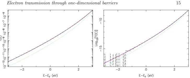
Fig. 2 compares the coefficient transmission T achieved when the energy of the

electron ranges from EF-3 eV to EF+3 eV (EF=10 eV). The figure compares the results

(7)

expression 1, by the transfer-matrix technique (TM), by the continued-fraction technique (CF) and by the simple JWKB approximation. For D=1 nm, the TM and CF results turn out to be in excellent agreement with each other and with the analytical expression 1. The continued-fraction technique presents however numerical instabilities for D=1.5

nm. These instabilities appear systematically when T is less than 10−15_{. The reason}

comes from the fact the transmission coefficient TFC = 1 −

¯ ¯ ¯(R−₀ − R−1)/(R−1− R0+) ¯ ¯ ¯2

is computed from a representation of the numbers R−1, R0− and R+0 that is limited to

52 binary digits for their mantissa (this corresponds to a representation with 16 decimal digits). The transfer-matrix technique on the other hand keeps stable over the whole range of conditions. It is for that reason that we use it as reference when analytical results are not available.

The simple JWKB approximation T = exp[−G] turns out to provide transmission coefficients that are systematically smaller than the exact quantum-mechanical result by

a factor that ranges between 1.5 and 4. The effective prefactor Peff to use in the Landau

and Lifschitz formula T = Peffexp[−G] in order to match the quantum-mechanical

result is represented in Fig. 3. The results correspond to a length D of 0.5, 1, 1.5

and 2 nm. The prefactor Peff that corresponds to these square barriers is essentially

independent of the length D. For E=10 eV, Peff takes the value of 3.424. These

conclusions are in excellent agreement with those achieved by Forbes.[20] According to Forbes, the prefactor to consider for the square barrier considered here is given by

Peff(E) = 16(E − VI)(V − E)/(V − VI)2 (using our notations and within the assumption

that G À 1). This result is indeed independent of the length D of the barrier. For E=10 eV, the expression given by Forbes provides the value of 3.424, which is in perfect agreement with our numerical result.

3.2. Application to triangular barriers

We now consider a triangular barrier, which is actually the barrier considered in the original paper by Fowler and Nordheim for modeling the emission achieved from a flat

metal.[2] We assume that a bias Vext of 1000 V is applied across Region II (this large

value aims at reducing the effects of considering that the potential energy in Region III is constant instead of varying with z as in Region II). The slope of the triangular barrier is determined by the field F that characterizes Region II and we have accordingly D = Vext/F for the length of this region. We take as previously EF=10 eV and φ=4.5

eV. We then define VI = 0, V (z) = EF + φ − eF z and VIII = EF + φ − eVext for the

potential energy in respectively Region I, II and III. The energy E for the electrons is

given by E = EF, which corresponds to the Fermi level of Region I.

Fig. 4 represents the transmission coefficient T for a triangular barrier, when the field F is 5 V/nm and 10 V/nm (these values are typical in field electron emission). The figure compares the results achieved by the transfer-matrix methodology (TM), the continued-fraction technique (CF), the simple JWKB approximation T = exp[−G]

(8)

value required in order to match the TM result for an electron in Region I with normal

energy E equal to the Fermi energy EF (Peff=1.839 for F =5 V/nm and Peff=1.820 for

F =10 V/nm). These results demonstrate that the JWKB result is smaller than the

quantum-mechanical result by a typical factor of 1.8 for an electron with E = EF. The

approximation that consists in evaluating the transmission coefficient by the formula T = Peffexp[−G], where Peff is determined for an electron with E = EF, actually holds with a good accuracy for energies that do not exceed the Fermi energy by more than 1 eV.

Fig. 5 represents the prefactor Peff to use in the Landau and Lifschitz formula

T = Peffexp[−G] in order to match the quantum-mechanical result. Peff is given as a function of the normal energy E and for different values of the electric field F . The

prefactor Peff turns out to depend significantly on the electric field F , especially for

energies that are closer to the apex of the barrier. The values actually range from 0.9 to 2.0 for the conditions considered. It was established by Fowler and Nordheim[2]

that in conditions where G À 1, Peff should be given by the square root of the value

achieved for a square barrier, i.e. Peff(E) = 4

q

(E − VI)(VI+ EF+ φ − E)/(EF+ φ) in

our notations. For electrons with E = EF (VI = 0), this relation indeed provides a value

of 1.850, which is in good agreement with the value of 1.848 obtained for F =1 V/nm. For higher fields, we deviate from the condition G À 1 for which the previous relation

holds. For F =10 V/nm, we get a prefactor Peff of 1.820, which is smaller (by 1.6%)

than the value predicted by this analytical expression. 3.3. Application to the Schottky-Nordheim barrier

The barrier that is directly relevant to field-emission problems is the Schottky-Nordheim barrier V (z) = EF+ φ − eF z − _16π²1 ₀e

2

z, in which the last term accounts for the image

interaction that applies to electrons in Region II. This expression tends to −∞ when z → 0 and the transmission coefficient T actually fails to converge (for physical reasons) if V (z) is not cut. We therefore prevented V (z) from dropping below the reference

potential VIof the metal in Region I. This is certainly the most reasonable thing to do in

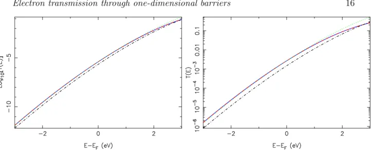
order to model the field-emission barrier and it corresponds indeed to the prescriptions of Murphy and Good[3] and Modinos[11] for this same issue. The way the potential energy in the field region actually connects to that in the metal is probably a delicate issue. Its impact on the field-emission currents is however not expected to be significant. Fig. 6 represents the transmission coefficient of the Schottky-Nordheim barrier for a field F of 5 V/nm and 10 V/nm. We compare the same methods as for the triangular barrier. The results achieved by the transfer-matrix technique and the continued fraction technique turn out to be in perfect agreement with each other. The JWKB approximation provides a reasonable estimation for the quantum-mechanical

result that corresponds to the field F of 5 V/nm (the prefactor Peff to use in the Landau

and Lifschitz formula T = Peffexp[−G] is 0.843 for an electron with E = EF and

(9)

values of the energy when we keep this value of Peff). For the field F of 10 V/nm, the results provided by the JWKB approximation and the Landau and Lifschitz formula

do not follow the quantum-mechanical result (the prefactor Peff to use in the Landau

and Lifschitz formula T = Peffexp[−G] is 0.631 for E = EF and this formula does not

account accurately for the transmission achieved for other values of the normal energy if

Peff is not adapted). The JWKB approximation and the Landau and Lifschitz formula

actually fail because the normal energy E is sufficiently close to the apex of the barrier. The Fröman and Fröman formula T = P exp[−G]/{1 + P exp[−G]} is better suited, in principle, to describe these situations in which the transmission coefficient T is close to 1.[20, 29] The result obtained using the Fröman and Fröman formula with P =0.721 is also included in Fig. 6 (this value of P is that required in order to match the

transfer-matrix result for E = EF; it is different from the effective prefactor Peff=0.631 to use in

the Landau and Lifschitz formula). The results achieved with the Fr¨oman and Fr¨oman formula are indeed closer to the exact result than those achieved with the Landau and Lifschitz formula. They deviate however immediately from the exact result as soon as the energy changes from the value for which the prefactor P is calculated.

Since the JWKB approximation is so widely used, even at the level of fundamental

theories relevant to field emission,[4, 3] it is useful to represent the correction factor Peff

to consider in the Landau and Lifschitz formula T = Peffexp[−G] in order to match

the exact quantum-mechanical result. This is done in Fig. 7, where we represented the

prefactor Peff to consider in order to get this exact result. The results are presented as a

function of the energy E, for different values of the electric field F . The different curves

show an inflection at the critical field Fcrit = 4π²0φ

2

e3 for which the apex of the barrier

corresponds to the Fermi level of the metal in Region I (this inflection also appears for the prefactor P that is relevant to the Fr¨oman and Fr¨oman formula). For fields F that are higher than this critical value, the electrons at the Fermi level of the metal can actually escape to the vacuum by ballistic motion over the barrier. A realistic metal would not sustain this regime and the conditions that are relevant to practical problems

correspond to F < Fcrit. In this range of field values, Peff ranges between 0.283 and

1.469 for the conditions considered. These values are smaller than those corresponding to the triangular barrier. They are indicative of the accuracy one can expect from field-emission models that rely on the simple JWKB approximation.

The results presented so far correspond to a work function φ of 4.5 eV for the metal

in Region I. In Fig. 8, we represented the prefactor Peff to consider in the Landau

and Lifschitz formula when we let the work function take values between 1 and 5 eV.

The representation is restricted to fields F that keep below Fcrit = 4π²0φ

2

e3 . These Peff

values are those to consider for electrons with E = EF in order get the exact

quantum-mechanical result for their transmission T = Peffexp[−G] through the surface barrier.

The normal energy at which these Peff values are calculated corresponds to that usually

considered in field-emission theories. Within the approximation that the same Peff could

be used for the different energies that contribute to the field-emission current, Fig. 8 would actually represents the correction factor to consider in order to get a more exact

(10)

emission current (the standard Fowler-Nordheim equation relies indeed on the simple

JWKB approximation; if JFN is the current density predicted by this equation, Peff.JFN

would represent a better approximation for this current density). As demonstrated in

this article, Peff however depends on the energy E and future work will be necessary

to determine the correction factor to consider with the Fowler-Nordheim equation. For

the conditions considered in Fig. 8, Peff ranges between 0.283 and 0.984. It thus shows

that the currents predicted by models that rely on the simple JWKB approximation over-estimate the currents one would obtain from a flat metal by a factor that can reach

values of the order of 2-3 for fields F that are close to the critical value Fcrit. This issue

will be addressed with more details in future work.

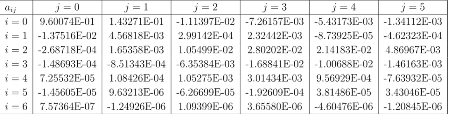
Before concluding this work, we provide a polynomial adjustment for the data

represented in Fig. 8. The effective prefactor Peff to use in the Landau and Lifschitz

formula T = Peffexp[−G] can be well represented by the best-fit expression Peff =

P₆

i=0

P₅

j=0aijXiYj, where X = F −1.7 with F the external field in V/nm and Y = φ−4.9

with φ the work function in eV. The coefficients aij of this adjustment are given in

Table 1. This expression applies for external fields F that keep below Fcrit = 4π²0φ

2

e3 . It is subject to the restrictions 1 V/nm ≤ F ≤ 10 V/nm and 3 eV ≤ φ ≤ 5 eV. For this range of parameters, this best-fit expression of the results provided by the TM

methodology is characterized by a maximum absolute error of 2.2 × 10−3 _{and by a mean}

error of 2.1 × 10−4_{. The reader can contact the author to obtain polynomial expressions}

that cover a wider range of parameters or to obtain the TM routines used for these calculations.

4. Conclusion

This article addressed the quantum-mechanical calculation of the electronic transmission through one-dimensional barriers that are relevant to field-emission problems. We compared in particular the results provided by the simple JWKB approximation, the continued-fraction technique and the transfer-matrix methodology for the case of square, triangular and Schottky-Nordheim barriers. The study confirmed that the simple JWKB

approximation must be completed by an effective prefactor Peff (thus yielding the

Landau and Lifschitz expression T = Peffexp[−G] for the transmission coefficient) in

order to match the exact quantum-mechanical result. For conditions that are typical of field emission (Fermi energy of 10 eV, work function of 4.5 eV and external field of 5

V/nm for the triangular and Schottky-Nordheim barriers), we have typically Peff ' 3.4

for square barriers, Peff ' 1.8 for triangular barriers and Peff ' 0.84 for the

Schottky-Nordheim barrier (these values are relevant to electrons with a normal energy equal

to the Fermi energy). With fields F that range between 1 V/nm and 10 V/nm, Peff

actually takes values between 0.91 and 0.63 for the Schottky-Nordheim barrier. If we

allow the work function φ to take values between 1 and 5 eV, Peff then ranges between

0.28 and 0.98. As observed by Forbes, the prefactor Peff is smaller for ”smooth” (ideal)

(11)

as long as F does not exceed the critical field Fcrit that cancels the surface barrier for

the normal energy E considered, we observe that Peff decreases with the normal energy

E of the electrons and with the strength of the field F . It increases with the work

function φ. The smaller values achieved for Peff actually correspond to the conditions

for which T ' 0.5, which corresponds to F ' Fcrit. These results are important in the

context of field emission since applications will actually tend to these conditions (they correspond indeed to higher emissions of current). The prediction of these currents often relies on the Fowler-Nordheim equation, which depends in turn on the JWKB approximation. This study however shows that this approximation deviates from the

exact quantum-mechanical result by a factor Peff that can be as small as 0.28 for the

conditions considered. The Fowler-Nordheim equation thus over-estimates the current achieved from a flat metal by a factor that can reach values of the order of 2-3 for fields F that are close to their critical value. This may affect any analysis of field-emission data that is based on the Fowler-Nordheim equation. This issue will be addressed with more details in future work.

Acknowledgments

This work was funded by the National Fund for Scientific Research (FNRS) of Belgium. The author acknowledges the use of the Inter-university Scientific Computing Facility (ISCF) of Namur. The author is grateful to R.G. Forbes for valuable suggestions and references regarding this work.

Appendix: The transfer-matrix methodology for the electronic transmission through arbitrary one-dimensional barriers

Let VI and VIII refer to the constant values of the potential energy in Region I (z ≤ 0)

and Region III (z ≥ D). The intermediate Region II (0 ≤ z ≤ D) is characterized by an arbitrary potential energy V (z) and we seek at determining the transmission of electrons with an energy E through this barrier.

The boundary states in Regions I and III are given respectively by Ψ±

I = e±ikIz and

Ψ±

III = e±ikIIIz, where kI = q 2m ¯ h2(E − VI) and kIII = q 2m ¯

h2(E − VIII). The transfer-matrix

methodology actually provides scattering solutions of the form

Ψ+ z≤0= Ψ+_I + S−+Ψ_I− z≥D= S++Ψ+_III, (A.1)

Ψ− z≤0_{= S}−−_Ψ+ I

z≥D

= Ψ−

III+ S+−Ψ+III, (A.2)

which correspond to incident states in respectively Regions I and Region III. The first solution, Eq. A.1, is actually that required in order to compute the transmission coefficients considered in this article. The presentation will therefore focus on the establishment of this solution only.

(12)

establishing an intermediate solution Ψz≤0= AIΨ+I + BIΨ−I

z≥D

= Ψ+

III, (A.3)

which corresponds to an outgoing state Ψ+

III in Region III. In order to determine the

coefficients AI and BI, one needs to propagate the values of Ψ(z) and dΨ(z)_dz from z = D,

where these values are perfectly defined, to z = 0. This is done by assuming that the potential energy V (z) in Region II varies in steps between z = 0 and z = D. If we take N steps of length ∆x = D/N and define zl = l∆z, we actually assume that the potential

energy takes the constant value Vl = [V (zl−1) + V (zl)]/2 in each step zl−1 ≤ z ≤ zl,

where l = 1, . . . , N.

The wave function Ψ(z) and its derivative dΨ(z)_dz take then in each step the analytical

expressions Ψ(z) = Aleiklz + Ble−iklz, (A.4) dΨ(z) dz = ikl(Ale iklz_{− B} le−iklz), (A.5) where kl = q 2m ¯

h2(E − Vl) (to keep concise, we allow at this point kl to be imaginary if

E < Vl). If the values of Ψ(zl) and dΨ(z_dzl) are known, one has

Al = 1 2e −iklzl " Ψ(zl) + 1 ikl dΨ(zl) dz # , (A.6) Bl = 1 2e iklzl " Ψ(zl) − 1 ikl dΨ(zl) dz # , (A.7)

which enables Ψ(zl−1) and dΨ(z_dzl−1) to be calculated through Eqs A.4 and A.5.

To implement the algorithm, one can define a vector Xl whose first component

X1

l contains the numerical value of Ψ(zl) and whose second component Xl2 contains

the derivative dΨ(zl)

dz . The full procedure consists then in defining XN1 = eikIIID and

X2

N = ikIIIeikIIID. The propagation from z = D to z = 0 is achieved by applying for

l = N, . . . , 1 the relation Ã X1 l−1 X2 l−1 ! = Ã cos(kl∆z) − sin(kl∆z)/kl klsin(kl∆z) cos(kl∆z) ! Ã X1 l X2 l ! , (A.8) when E > Vl (kl = q 2m ¯ h2(E − Vl)), the relation Ã X1 l−1 X2 l−1 ! = Ã cosh(Kl∆z) − sinh(Kl∆z)/Kl −Klsinh(Kl∆z) cosh(Kl∆z) ! Ã X1 l X2 l ! , (A.9) when E < Vl (Kl = q 2m ¯

h2(Vl− E)), or the relation

Ã X1 l−1 X2 l−1 ! = Ã 1 −∆z 0 1 ! Ã X1 l X2 l ! , (A.10)

when E = Vl. We have finally that

AI= 1 2 · X1 0 + 1 ikI X2 0 ¸ , (A.11) BI= 1 2 · X1 0 − 1 ikI X2 0 ¸ , (A.12)

(13)

which enables S++ _{and S}−+ _{to be calculated from S}++_{= 1/A}

I and S−+= BI/AI. The ”transmission coefficient” of the potential barrier V (z) at the energy E is finally given by

T = kIII kI

|S++_|2_. _(A.13)

This transmission coefficient T relates the current density Jin, which is associated with

the incident state Ψ+

I in Region I, to the current density Jout = T.Jin, which is associated

with the transmitted state S++_Ψ+

III in Region III.

This procedure provides the exact quantum-mechanical result for the electronic transmission through a barrier that varies in steps in the region 0 ≤ z ≤ D. The accuracy of this approximation can be controlled by letting ∆z → 0. For three-dimensional problems, it is necessary to apply the layer-addition algorithm presented by Pendry[30] in order to prevent the occurrence of numerical instabilities. This is explained with details in Ref. [31]. The adaptation of the techniques presented in this Appendix to the three-dimensional case can be found in Refs [25, 26, 27, 28].

References

[1] Xu NS and Huq SE 2005 Mat. Sci. Eng. R 48 47

[2] Fowler RH and Nordheim LW 1928 Proc. R. Soc. London Ser. A 119 173 [3] Murphy EL and Good RH 1956 Phys. Rev. 102 1464

[4] Good RH and M¨uller EW 1956 Handbuch der Physik (S. Flugge, Springler Verlag, Berlin) 21 176 [5] Young RD 1959 Phys. Rev. 113 110

[6] Stratton R 1964 Phys. Rev. 135 A764

[7] Nagy D and Cutler PH 1969 Phys. Rev. 186 651 [8] Swanson LW and Crouser LC 1967 Phys. Rev. 163 622 [9] Gadzuk JW and Plummer EW 1973 Rev. Mod. Phys. 45 487

[10] Miskovsky NM, Park SH, He J and Cutler PH 1993 J. Vac. Sci. Technol. B 11 366 [11] Modinos A 2001 Solid State Electron 45 809

[12] Forbes RG and Deane JHB 2007 Proc. R. Soc. A 463 2907 [13] Forbes RG 2008 J. Vac. Sci. Technol. B 26 788

[14] Cutler PH, He J, Miskovsky NM, Sullivan TE and Weiss B 1992 J. Vac. Sci. Technol. B 11 387 [15] Jeffreys H 1925 Proc. London Math. Soc. 23 428

[16] Wentzel G 1926 Z. Phys. 38 518 [17] Kramers HA 1926 Z. Phys. 33 828 [18] Brillouin L 1926 Compt. Rend. 183 24 [19] Kemble EC 1935 Phys. Rev. 48 549 [20] Forbes RG 2008 J. Appl. Phys. 103 114911

[21] Landau LD and Lifschitz EM Quantum Mechanics (Pergamon, Oxford, 1958) [22] Vigneron J-P and Lambin P 1980 J. Phys. A: Math. Gen. 13 1135

[23] Nguyen HQ, Cutler PH, Feuchtwang TE, Miskovsky NM and Lucas AA 1985 Surf. Sci. 160 331 [24] Mayer A and Vigneron J-P 1999 Ultramicroscopy 79 35

[25] Mayer A and Vigneron J-P 1997 Phys. Rev. B 56 12599 [26] Mayer A and Vigneron J-P 1999 Phys. Rev. B 60 2875

[27] Mayer A and Vigneron J-P 1999 J. Vac. Sci. Technol. B 17 506

[28] Mayer A, Chung MS, Weiss BL, Miskovsky NM and Cutler PH 2008 Phys. Rev. B 78 205404 [29] Fr¨oman H and Fr¨oman PO JWKB Approximation: Contributions to the Theory (North-Holland,

(14)

[30] Pendry JB 1994 J. Mod. Opt. 41 209

(15)

aij j = 0 j = 1 j = 2 j = 3 j = 4 j = 5

i = 0 9.60074E-01 1.43271E-01 -1.11397E-02 -7.26157E-03 -5.43173E-03 -1.34112E-03 i = 1 -1.37516E-02 4.56818E-03 2.99142E-04 2.32442E-03 -8.73925E-05 -4.62323E-04

i = 2 -2.68718E-04 1.65358E-03 1.05499E-02 2.80202E-02 2.14183E-02 4.86967E-03

i = 3 -1.48693E-04 -8.51343E-04 -6.35384E-03 -1.68841E-02 -1.00688E-02 -1.46163E-03

i = 4 7.25532E-05 1.08426E-04 1.05275E-03 3.01434E-03 9.56929E-04 -7.63932E-05

i = 5 -1.45605E-05 9.63213E-06 -6.26699E-05 -1.92609E-04 3.81486E-05 3.43046E-05 i = 6 7.57364E-07 -1.24926E-06 1.09399E-06 3.65580E-06 -4.60476E-06 -1.20845E-06

Table 1. Coefficients aijof the polynomial adjustment Peff =

P₆ i=0

P₅

j=0aijXiYjfor the effective prefactor Peff to use in the Landau and Lifschitz formula T = Peffexp[−G]

for the transmission through a Schottky-Nordheim barrier. In this expression, X =

F − 1.7 with F the external field in V/nm and Y = φ − 4.9 with φ the work function

in eV. This expression is restricted to F < 4π²0_e3φ2, 1 V/nm ≤ F ≤ 10 V/nm and

3 eV ≤ φ ≤ 5 eV.

Figure 1. (Color online) Potential energy for the case of a square barrier (solid), a triangular barrier (dashed) and a Schottky-Nordheim barrier (dot-dashed). The representation corresponds to a Fermi energy EF of 10 eV, a work function φ of 4.5

(16)

Figure 2. (Color online) Transmission coefficient T for a square barrier of height

V =14.5 eV and of length D=1 nm (left) and 1.5 nm (right). T is computed from its

analytical expression (solid), the transfer-matrix technique (dashed), the continued-fraction technique (dot-dashed) and the simple JWKB approximation (dotted). The reference EF for the energy of the electrons is 10 eV.

Figure 3. (Color online) Prefactor Peff to use in the Landau and Lifschitz formula T = Peffexp[−G] in order to match the quantum-mechanical result for the transmission

through a square barrier with a height V of 14.5 eV and a length D of 0.5 nm (solid), 1 nm (dotted), 1.5 nm (dot-dashed) and 2 nm (dotted). The reference EFfor the energy

(17)

Figure 4. (Color online) Transmission coefficient T for a triangular barrier corresponding to a field F of 5 V/nm (left) and 10 V/nm (right). The Fermi level of the metal in Region I is taken as reference for the normal energy E of the electrons.

T is computed from the transfer-matrix technique (solid), the continued-fraction

technique (dashed), the simple JWKB approximation T = exp[−G] (dot-dashed) and the Landau and Lifschitz formula T = Peffexp[−G] (dotted), where Peff=1.839 (left)

and Peff=1.820 (right). The calculations correspond to a Fermi energy of 10 eV and a

work function of 4.5 eV.

through a triangular barrier corresponding to a field F that goes from 1 V/nm to 10 V/nm (downwards, by increments of 1 V/nm). The Fermi level of the metal in Region I is taken as reference for the normal energy E of the electrons. The calculations correspond to a Fermi energy of 10 eV and a work function of 4.5 eV.

(18)

Figure 6. (Color online) Transmission coefficient T for a Schottky-Nordheim barrier corresponding to a field F of 5 V/nm (left) and 10 V/nm (right). The Fermi level of the metal in Region I is taken as reference for the normal energy E of the electrons.

T is computed from the transfer-matrix technique (solid), the continued-fraction

technique (dashed), the simple JWKB approximation T = exp[−G] (dot-dashed) and the Landau and Lifschitz formula T = Peffexp[−G] (dotted), where Peff= 0.843 (left)

and Peff=0.631 (right). The figure corresponding to F =10 V/nm also includes the

result achieved using the Fr¨oman and Fr¨oman formula T = P exp[−G]/{1+P exp[−G]} (solid, as indicated), where P =0.721. The calculations correspond to a Fermi energy of 10 eV and a work function of 4.5 eV.

through a Schottky-Nordheim barrier corresponding to a field F that goes from 1 V/nm to 10 V/nm (downwards, by increments of 1 V/nm). The Fermi level of the metal in Region I is taken as reference for the normal energy E of the electrons. The calculations correspond to a Fermi energy of 10 eV and a work function of 4.5 eV.

(19)

through a Schottky-Nordheim barrier when the energy of the electrons corresponds to the Fermi level of the metal. The results are represented as a function of the field

F and work function φ. The representation is restricted to fields F that keep below Fcrit= 4π²0φ

2