RESEARCH OUTPUTS / RÉSULTATS DE RECHERCHE
Author(s) - Auteur(s) :
Publication date - Date de publication :
Permanent link - Permalien :
Rights / License - Licence de droit d’auteur :
Bibliothèque Universitaire Moretus Plantin
Institutional Repository - Research Portal
Dépôt Institutionnel - Portail de la Recherche
researchportal.unamur.be
University of Namur
Does Training Lead to the Formation of Modules in Threshold Networks?
Nicolay, Delphine; Andrea, Roli; Carletti, Timoteo
Published in:
Proceedings of ECCS 2014
Publication date:
2016
Document Version
Publisher's PDF, also known as Version of record
Link to publication
Citation for pulished version (HARVARD):
Nicolay, D, Andrea, R & Carletti, T 2016, Does Training Lead to the Formation of Modules in Threshold
Networks? in Proceedings of ECCS 2014: European Conference on Complex Systems. Springer Proceedings in Complexity, Springer, pp. 181-192, eccs'14, Lucca, Italy, 22/09/14.
General rights
Copyright and moral rights for the publications made accessible in the public portal are retained by the authors and/or other copyright owners and it is a condition of accessing publications that users recognise and abide by the legal requirements associated with these rights. • Users may download and print one copy of any publication from the public portal for the purpose of private study or research. • You may not further distribute the material or use it for any profit-making activity or commercial gain
• You may freely distribute the URL identifying the publication in the public portal ? Take down policy
If you believe that this document breaches copyright please contact us providing details, and we will remove access to the work immediately and investigate your claim.
Does Training Lead to the Formation of Modules
in Threshold Networks?
D. Nicolay1, A. Roli2, and T. Carletti1
1
Department of Mathematics and naXys, University of Namur, Belgium
2 Department of Computer Science and Engineering (DISI), University of Bologna,
Campus of Cesena, Italy
Abstract. This paper addresses the question to determine the necessary conditions for the emergence of modules in the framework of artificial evolution. In particular, threshold networks are trained as controllers for robots able to perform two different tasks at the same time. It is shown that modules do not emerge under a wide set of conditions in our experimental framework. This finding supports the hypothesis that the emergence of modularity indeed depends upon the algorithm used for artificial evolution and the characteristics of the tasks.
1
Introduction
Modularity is a widespread feature of biological and artificial networks such as animal brains, protein interactions and robot controllers. This feature makes networks more easily evolvable, i.e. capable of rapidly adapting to new environ-ments and offers computational advantages. Indeed, an intuitive idea is that it is easier and less costly to rewire functional subunits in modular networks. Despite its advantages, modularity remains a controversial issue, with disagreement con-cerning the nature of the modules that exist as well as over the reason of their appearance in real networks [16]. Moreover, there is no consensus concerning the conditions for their emergence.
Whereas most hypotheses assume indirect selection for evolvability, Bulli-naria [3] suggests that the emergence of modularity might depend on different external factors such as the learning algorithm, the effect of physical constraints and the tasks to learn. Clune et al. [4] also claimed that the pressure to reduce the cost of connections between network nodes causes the emergence of modular networks. On their side, Kashtan and Alon [8] found that switching between several goals leads to the spontaneous evolution of modular networks.
In this work, we study the emergence of modularity in the field of evolu-tionary robotics. First of all we remark that there is not a uniquely accepted definition of modularity; moreover, the existence of many different definitions, each one appropriate for different levels of abstraction [6, 13], makes this ques-tion even more intricated. We thus decided to analyse our results by considering two kinds of modularity, namely topological modularity, which is a measure of the density of links inside modules as compared to links between modules, and
functional modularity, which groups together neurons that have similar dynamic behaviours.
The case under study consists in learning conflicting tasks where robots con-trollers are realised as neural networks. The learning phase is performed using a genetic algorithm that optimises both network structure and weights. Our start-ing workstart-ing assumption is that only two conditions are needed for the emergence of modularity. Firstly, at least two tasks should be learnt. Secondly, the learn-ing must be incremental, i.e. the modifications in both topology, weights and activation thresholds must be gradual and the structure of the networks can not be too strongly modified in one step. Let us also remark that the outcome of the learning process is path dependent as the learning algorithm is heuristic. Because the results obtained from the first assumption were unsatisfactory we decided to improve our working assumption by considering: switching between the tasks learning, cost of the connections and cost of the nodes, and thus to study their impact on the networks evolution.
Because we were not able to detect any kind of modules in all the performed experiments, our findings support the hypothesis that the emergence of modu-larity is not exclusively conditioned by the learning conditions but also depends upon the algorithm used for artificial evolution and the characteristics of the tasks. Furthermore, we conjecture that the computational nature of the tasks, namely combinatorial or sequential – i.e. requiring memory to be accomplished – may also play a role in the emergence of modularity.
The paper is organised as follows. In section 2, we present our experimental settings, namely our model of networks, the tasks the robot has to perform and our learning algorithm. Experiments and results are described in section 3. Section 4 concludes the contribution with a summary of our results.
2
Model and Tasks Description
The abstract application we focussed on is based on the experimental framework introduced by Beaumont in [1]. Virtual robots are trained to achieve two different tasks in a virtual arena. This arena is a discretised grid with a 2 dimensional torus topology on which robots are allowed to move into any neighbouring cell at distance 1 at each displacement. Assuming the arena possesses one global maximum, the aim of the first task, task A in the following, is to reach and to stay on this global maximum. The second task, task B, consists in moving incessantly by avoiding zones where robots lose energy, called “dangerous zones”. Let us observe that such tasks are conflicting, because the first task will imply the robot to reach the peak and stay there, while the second would rather make the robot to wander around the arena.
The robots we considered have 17 sensors and 4 motors. The 9 first sensors check the local slope, that is the heights of the cell on which the robot is located and the cells around it. The 8 others are used to detect the presence of “dangerous zones” on the cells surrounding the robots. The 4 motors control the movements of robots, i.e. moving to the north-south-east and west and their combinations.
We used neural networks [11, 12] as robot controllers. They are made of 43 nodes: 17 inputs, 4 outputs and 22 hidden neurons. This number is large enough to let sufficient possibilities of connections to achieve the tasks, but it is still low to use reasonably level of CPU resources. The topology of these networks is completely unconstrained, except for self-loops that are prohibited. The weights and thresholds are real values between -1 and 1. The states of the neurons are binary and the updates are performed following the perceptron rule:
∀j ∈ {1, . . . , N } : xt+1j = 1 if kin j P i=1 wt jixti− θ ≥ 0 0 otherwise
where kinj is the number of incoming links in the j–th neuron, θ the threshold of the neuron, and wt
jiis the weight, at time t, of the synapse linking i to j.
The robot controllers, i.e., the neural networks, are trained to achieve both tasks. This training consists in finding the suitable topology and the appropriate weights and thresholds to obtain neural networks responsible for good robot’s behaviour. We resort to genetic algorithm [5, 7], for short GA in the following, to perform this optimisation heuristically. Let us observe that we can not use here a standard backpropagation algorithm, looking at the computed output and the required one, to fix the weights to minimise such difference. In fact the behaviour we wish to optimise depends on the full path followed by the robot, so act on the weights aimed at minimising the right solution – that we yet don’t know – with the followed path would result in an optimisation problem per se. This GA is real-valued, as genotypes encode weights and thresholds of the networks. The selection is performed by a roulette wheel selection. The operators are the classical 1-point crossover and 1-inversion mutation. Their respective rates are 0.9 and 0.005, while the population size is 100 and the maximum number of generations is 50 000. To ensure the legacy of best individuals, the population of parents and offsprings are compared at each generation before keeping the best individuals among both populations. New random individuals (one-tenth of the population size) are also introduced at each generation by replacing worst individuals to avoid premature convergence.
Further details on the application and the model have already been presented in previous works [9, 10].
3
Experiments and Results
At the first stage of the experimental set up, we designed experiments that respect the two conditions that we assumed to be necessary for the emergence of modularity. These conditions are to learn more than one task and to modify the networks gradually during the training. As our optimisation process is stochastic, we performed 10 independent replicas of each experiment and in the rest of the paper we report results in terms of such averages.
For each experiment, we analysed two kinds of modularity. The first one is topological modularity, a measure of the density of links inside modules as
compared to links between modules. We use the Louvain method [2] to study this modularity. The second one is functional modularity, which groups together neurons that have similar dynamic behaviours. The functional modularity is analysed by using the dynamical cluster index [14, 15], which makes it possi-ble to identify subsets of variapossi-bles that are integrated among themselves and segregated with the rest of the system. The analysis is made by collecting the multidimensional time series composed of network’s variables values during the execution of the task. For details on this method, we refer the interested reader to [15].
3.1 Initial Conditions
We originally considered three ways to train the robot. First, it is trained on the two tasks at the same time (i). In this case, the fitness is obtained by averaging the fitness of each task using equal weights. Second, the robot is trained first on one task and then on both (ii). The GA is first applied with one fitness function – the one related to the task under scrutiny – and then once again with the weighted sum of the two. The third possibility consists in training two smaller networks so as to accomplish each task separately, then combine the networks by adding a small extra network and train the new larger network (called juxtaposition in the following), using as fitness once again the weighted sum of the fitness for each task, as in case (i). In terms of robot’s performance, these three learning ways are equivalent with final fitness value around 0.75 (observe that we work with a normalised fitness in [0, 1]).
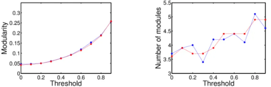
To study the topological modularity in case (i) and (ii), we analysed the modularity and the number of modules got by the Louvain method when we kept strong enough connections, i.e connections whose absolute values of the weights are superior to a fixed threshold value. The method thus returns a modularity value in [0, 1], where 0 means that there are no modules and 1 that there are no interactions between modules. We compared the results of our evolved networks with those of random networks used as null hypothesis. These random networks have the same features of our networks, i.e. the same number of nodes, the same density of connections and the same distribution of weights. Figure 1 presents this comparison in case (i) for different threshold values. We can observe that evolved and random networks behave similarly and hence we can conclude that the evolved networks are not modular. We obtained analogous results in case (ii) (data not shown).
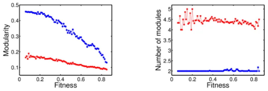
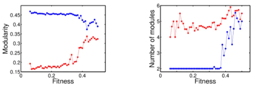
The case juxtaposition is analysed in a different way. Indeed, initial networks are modular as they consist in the combination of two smaller networks, each trained to accomplish one task, and a small extra network. Thus, we decided to observe the evolution of topological modularity as a function of the increase of robot’s performance. The evolution of trained networks is presented in Fig. 2 for the modularity (left panel) and for the number of modules (right panel). Results are also compared with those of random networks with the same features as previously. We can notice that the results obtained for evolved and random networks are significantly different. We also found that, in 9 simulations out
of 10, the number of modules doesn’t change during the optimisation (data not shown). Each module is made by one initial small network (able to perform a given task), while the nodes of the extra small network are shared between the two main modules. The size of these modules is sometimes slightly modified when one node of the extra network jumps from one module to the other. Although the number of modules is almost constant, we can observe a strong decrease of modularity along the optimisation process.
Fig. 1. Comparison of the topological modularity between evolved networks in case (i) and random networks. Blue (on line) circles represent the evolved networks, while red (on line) squares represent the random networks used as comparison. Left panel: Mod-ularity. Right panel: Number of modules. In both cases, the modularity is computed on networks whose weights have been set equal to 0 if their absolute value is below a given threshold. Results are similar for evolved and random networks, which leads to the conclusion that the evolved networks are not topologically modular.
Following these results, we concluded that none of the training schemes leads to topologically modular networks. In the case juxtaposition, it even seems to make disappear the initial modularity, as long as the modularity score is consid-ered.
Regarding functional modularity, no clear modules are found in all the anal-ysed cases. The search for functional modules returned either a subset composed of all but a few nodes – i.e. almost all nodes are involved in the processing – or few small subsets with no statistical significance. For this reason we decided not to show data. When the robot is trained according to scheme (ii), i.e. sequential learning, naive modules form in the first phase of the training, as only one part of the sensors is stimulated. Nevertheless, these modules disappear when the robot is subsequently trained to accomplish both the tasks. Furthermore, the same results as for the topological analysis are observed in the case juxtaposi-tion, showing that the initial modules tend to be blended together in the final training phase.
The results returned by the analysis of functional modularity strengthen those on the topology, as they show that not only the networks have no appar-ent modules, but that they do not even show clusters of nodes which work in coordinated way and corresponding to either of the two tasks.
Fig. 2. Evolution of the topological modularity as a function of the fitness increase for the evolved networks in the case juxtaposition and for random networks. Blue circles represent the evolved networks while red squares represent the random networks. Left panel: Modularity. Right panel: Number of modules. We clearly observe that modularity decreases along the training process even if the number of modules is almost steady.
3.2 Improving the Experimental Setting
Results presented in the previous section do not support the presence of mod-ules. To check if this is due to our main assumptions, we consider additional conditions that could be important for their emergence according to the liter-ature. These conditions are the alternance between different goals, the penalty on the number of connections and the decrease of the number of hidden nodes. Switching between Goals
We first followed the suggestion of Kashtan and Alon that switching between different goals is important for the emergence of modules. We considered a fourth training scheme (iv) in which the target task is alternated every 100 generations. In preliminary tests, we also considered to alternate every 20 or 50 generations but the simulations with 100 gave us the best robot performance. Even if one particular task is trained in each epoch, all sensors are stimulated. Otherwise, robots can accomplish both tasks but not simultaneously. The results obtained by the simulations of this fourth scheme are similar to those of previous schemes. Indeed, the robot performance is also around 0.75 and the analysis of the topo-logical modularity leads us to similar results to those presented in Fig. 1. The same also holds true for functional modularity, with analogous results to the previous cases.
Cost of Connections
Bullinaria [3] as well as Clune et al. [4] claimed that the penalty on the number of connections is essential for the formation of modules. So, we added this penalty for each of the four training schemes considered previously. The penalty con-tributes to 3/10 of the average fitness in each experiment. In case (i), the weight of each task is reduced to 0.35 instead of 0.5. For the second scheme, robot is trained first on one task with the penalty on the number of connections. Then robot is trained on both tasks with the penalty as described for scheme (i). For
the juxtaposition scheme, the penalty is only added for the last phase of learning because if the penalty is also used while training the two smaller networks, the resulting fitness is too low (0.35 which is smaller than the half fitness of other experiments). For the case (iv), the penalty on the number of connections is con-sidered during the training of the two alternated task. Let us observe that the fitness described in this paragraph are only used for the training phase. Results are then analysed using robot’s performance corresponding to the fitness of the two tasks summed using equal weights, in this way we can compare them with the former ones.
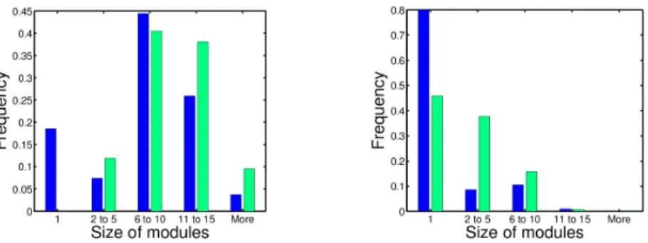
When we analysed topological modularity, we obtained similar results for scheme (i), scheme (ii) if the learning procedure starts with task B (avoid dan-gerous zones) and scheme (iv). Indeed, in these cases, the fitness is nearly the same than without the penalty on the number of connections. Moreover, the modularity is low (close to 0.1) while random networks with the same density of links and the same distribution of weights have comparable values ∼ 0.15. The difference appears in the number of modules that is slightly higher in evolved networks as shown in the left panel of Fig. 3, which shows the distribution of modules according to their size. Indeed, in trained networks, some modules con-sist of isolated nodes, i.e. nodes without any link with the rest of the network. Let us observe that this never happens in random networks.
Fig. 3. Comparison of the distribution of modules according to their size between evolved networks with penalty and random networks with the same density of links and distribution of weights. Blue bars represent the results for evolved networks while green bars represent those for the random networks. Left panel: Scheme (i). Right panel: Scheme (ii) when training starts with task A. The number of isolated nodes is significantly higher in evolved networks.
As the cost on the number of connections did not lead to the emergence of modules, we might suspect that the penalty that we had fixed was not strong enough to involve modularity. Nevertheless, we obtained similar results with a larger penalty of 0.5, which is a quite high value representing half of the fitness during the optimisation process.
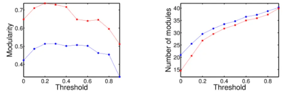
If we consider scheme (ii) when the first trained task is task A (reach the peak), the value of the fitness decreases slightly with an average value of 0.67. Moreover if we compare the modularity between these networks and random networks with the same features by keeping connections whose absolute values of weights are larger than a given threshold value (see Fig. 4), we can observe a significantly different behaviour. The value of the topological modularity is lower for evolved networks while their number of modules is higher. If we con-sider evolved networks without eliminating any connections (threshold of 0), we observe that the number of modules is ∼ 21, out of which ∼ 17 are isolated nodes for evolved networks, for random networks we got respectively ∼ 15 and ∼ 7. This high frequency of isolated nodes is also clearly apparent in the right panel of Fig. 3. We can explain such results by the simplicity of task A, which indeed requires few connections to be accomplished. When this task is trained alone with the penalty on the number of connections, we got networks with a high level of modularity and a high number of modules, most of which are isolated nodes, comprising non-stimulated inputs. As the penalty cost is always active in the second phase of learning, useless hidden nodes remain isolated, which leads to a higher modularity than for previously analysed training schemes.
Once we eliminated these isolated nodes, the analysis of evolved networks gives us similar results to those of our initial assumption.
Fig. 4. Comparison of topological modularity between evolved networks in case (ii), when the training starts with task A and random networks with the same features. Blue (on line) circles represent the evolved networks and red (on line) squares the random networks used as comparison. Left panel: Modularity. Right panel: Number of modules. Evolved networks have a slower rate of modularity than random networks but they contain more modules.
In the case juxtaposition, the mean fitness of simulations is 0.44, which is considerably smaller than for other experiments. Figure 5 shows the evolution of modularity according to the increase in robot’s performance. The decrease of modularity seems to be less important than without the penalty but the final fitness is lower. The difference that exists between the modularity of evolved net-works and random netnet-works significantly decreases during the learning process.
Following this experiment, we conclude that the penalty on the number of links allows to keep a level of modularity close to the initial one. Indeed, the decline in the number of connections leads to the emergence of isolated nodes that increases the modularity but to the detriment of robot’s performance. As for functional modularity, no significant groups of nodes are identified with co-ordinated behaviour.
Fig. 5. Evolution of the topological modularity as a function of the fitness increase in the case juxtaposition with penalty. Blue circles represent the evolved networks while red squares represent the random networks. Left panel: Modularity. Right panel: Num-ber of modules. The decrease of modularity is less important than in the case without penalty. Contrarily, the number of modules rises with the appearance of isolated nodes.
Number of Hidden Nodes
Another argument by Bullinaria [3] is that the number of hidden nodes plays a role in the emergence of modules. Indeed, modularity has more possibilities to appear if the number of hidden nodes is small. Thus, our last experimental settings consisted in decreasing the number of hidden nodes and testing if this can lead to the formation of modules in evolved networks. This case can be con-sidered as a very strong implementation of the previous analysis where, instead of removing one link we remove several links, i.e. all the ones connected to a given node. With this aim, we only considered the first training scheme (i).
We checked the dependence on the number of hidden nodes on robot perfor-mance and modularity. One would expect the perforperfor-mance to be very poor for very small number of hidden nodes – i.e. not enough to perform the required computation – then the performance should increase as long as the number of hidden nodes increases up to some number, beyond which no improvement is found. The robot performance is tested on the training set and on three differ-ent validation sets, i.e. scenarios robots never seen before. In the first two cases, we modify respectively the location of loss of energy zones and the shape of the surface to climb (position of the peak and slope of the surface). The last third case takes into account both modifications.
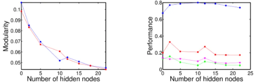
Results are presented in Fig. 6. The left and right panel respectively present the modularity and the robot performance according to the number of hidden
nodes. Modularity decreases when the number of hidden nodes increases and no functional modules have been detected. Regarding robot performance, we can-not observe significant decrease when the number of hidden nodes is small. Even more, the performance seems to be better in the validation phase for networks without any hidden node. This result may be explained by the fact that mem-ory is not needed to solve the problem and thus hidden nodes, responsible for information storage, are not relevant to accomplish the task. Observations are the same if we add the penality on the number of connections to the learning process.
In conclusion, also in this experiment no topological modularity is observed. Likewise, the analysis of functional modularity does not support the emergence of modules in these smaller networks.
Fig. 6. Evolution of robot’s performance and modularity according to the number of hidden nodes. Left panel: Modularity compared to the one of random networks with the same features. Modularity decreases when the number of hidden nodes rises. Right panel: Robot’s performance on the training set and on three validation sets. Blue (on line) circles represent the performance on the training set while red squares and green diamonds show respectively the performance on an arena whose the shape of the surface and the zones where robots lose energy have been modified. The magenta triangles represent the fitness when both modifications are performed. We can not observe significant differences of performance.
4
Conclusion
Modularity is a major factor of evolvability in biological and artificial networks. Nevertheless, it remains a controversial issue with disagreement over the suffi-cient conditions for the appearance of modules. This paper analyses the emer-gence of modularity in the context of evolutionary robotics by taking into account some of the most frequently used conditions in the literature. With this aim, two kinds of modularity are considered, namely the topological modularity and the functional modularity.
We assume that robot controllers, made of neural networks, are trained to fulfil two conflicting tasks. The learning process is a GA that modifies both structure and weights of the controllers. Our initial working assumption is that
the emergence of modularity only requires two conditions, namely the learning of at least two tasks and an incremental optimisation process. Faced with the unsatisfying results obtained by this first assumption, we considered supplemen-tary conditions such as switching between the tasks learning, penalising the cost of connections and decreasing the number of hidden nodes. However, contrary to results obtained in previous studies, we can not observe the emergence of topological and functional modularity whatever the conditions that we consider. Even more, under our initial assumptions, it seems that the learning phase leads to the disappearance of the initial modules. Our results suggest that tasks switching doesn’t modify our former ones. When we introduce a penalisation to the density of connections, the level of modularity is higher, but associated to the appearance of isolated nodes in the evolved networks. The reduction of the number of hidden nodes doesn’t lead to the emergence of modularity but brings us interesting results. Indeed, we can observe that hidden nodes do not seem to be needed to learn the tasks.
This fact suggests us a possible explanation of the absence of modularity and even a reduction of modularity as learning proceeds. In fact, neural networks composed of only input and output nodes cannot be modular. Indeed, outputs are shared among the tasks and not splitted as in the experiments of Clune. Thus, modular networks would imply that some inputs are disconnected from some outputs and this assumption seems hard to be satisfied because input signals are not correlated. Therefore, once we initialise the neural network with hidden nodes and links, we are adding an “unnecessary” structure resulting in some detectable modularity, which will be slowly removed by the learning phase (creating isolated nodes or making all the nodes to work together) and so finally decrease the network modularity. As a consequence, a possible clue to have modular structures to emerge because of a learning phase with (at least) two tasks is that they require memory to be accomplished.
Even if it provides more questions than answers, the conclusion of this study is promising as it extends the study of the emergence of modularity to another context. Modularity has already been studied in the field of evolutionary robotics but our research differs from previous studies in the choice of the learning al-gorithm and of the application. Indeed, we trained both structure and weights by a GA whereas weights are usually trained by a backpropagation algorithm. Likewise, our conflicting tasks are computationally more complex than tasks generally considered in other studies (classification tasks or what-where tasks). The absence of modularity in our case strengthens the claim of Bullinaria [3] that the emergence of modularity might depend on external factors such as the learning algorithm and the tasks to learn. Further work will address this issue in more depth.
Acknowledgements
This research used computational resources of the “Plateforme Technologique de Calcul Intensif (PTCI)”located at the University of Namur, Belgium, which is supported by the F.R.S.-FNRS.
This paper presents research results of the Belgian Network DYSCO (Dynamical Systems, Control, and Optimisation), funded by the Interuniversity Attraction Poles Programme, initiated by the Belgian State, Science Policy Office.
References
[1] M.A. Beaumont. Evolution of optimal behaviour in networks of boolean automata. Journal of Theoretical Biology, 165:455–476, 1993.
[2] V. D. Blondel, J-L. Guillaume, R. Lambiotte, and E. Lefebvre. Fast unfolding of communities in large networks. Journal of Statistical Mechanics: Theory and Experiment, 2008(10):P10008, 2008.
[3] J. A. Bullinaria. Understanding the emergence of modularity in neural systems. Cognitive Science, 31(4):673–695, 2007.
[4] J. Clune, J-B. Mouret, and H. Lipson. The evolutionary origins of modularity. Proceedings of the Royal Society b: Biological sciences, 280(1755):20122863, 2013. [5] K. Deb. Multi-Objective Optimization using Evolutionary Algorithms. John Wiley
& Sons Ltd, Chichester, 2008.
[6] D. C. Geary and K. J. Huffman. Brain and cognitive evolution: forms of modu-larity and functions of mind. Psychological bulletin, 128(5):667, 2002.
[7] D. E. Goldberg. Genetic Algorithms in Search, Optimization, and Machine Learn-ing. Addison-Wesley, 1989.
[8] N. Kashtan and U. Alon. Spontaneous evolution of modularity and network motifs. Proceedings of the National Academy of Sciences, USA, 102(39):13773– 13778, 2005.
[9] D. Nicolay and T. Carletti. Neural networks learning: Some preliminary re-sults on heuristic methods and applications. In A. Perotti and L. Di Caro, edi-tors, DWAI@AI*IA, volume 1126 of CEUR Workshop Proceedings, pages 30–40. CEUR-WS.org, 2013.
[10] D. Nicolay, A. Roli, and T. Carletti. Learning multiple conflicting tasks with artificial evolution. In Advances in Artificial Life and Evolutionary Computation, volume 445 of Communications in Computer and Information Science, pages 127– 139. Springer International Publishing, 2014.
[11] P. Peretto. An introduction to the modeling of neural networks. Alea Saclay. Cambridge University Press, Cambridge, 1992.
[12] R. Rojas. Neural networks: A systematic introduction. Springer, Berlin, 1996. [13] B. Seok. Diversity and unity of modularity. Cognitive Science, 30(2):347–380,
2006.
[14] M. Villani et al. The detection of intermediate-level emergent structures and patterns. In Advances in Artificial Life, ECAL, volume 12, pages 372–378, 2013. [15] M. Villani et al. The search for candidate relevant subsets of variables in complex
systems. Artificial Life, 2015. Accepted. Also available as arXiv:1502.01734. [16] G. P. Wagner, M. Pavlicev, and J. M. Cheverud. The road to modularity. Nature