Probabilistic Logical Models for Large-Scale Hybrid Domains

(1)

HAL Id: tel-01462085

https://hal.archives-ouvertes.fr/tel-01462085

Submitted on 18 Dec 2017

HAL is a multi-disciplinary open access

archive for the deposit and dissemination of

sci-entific research documents, whether they are

pub-lished or not. The documents may come from

teaching and research institutions in France or

abroad, or from public or private research centers.

L’archive ouverte pluridisciplinaire HAL, est

destinée au dépôt et à la diffusion de documents

scientifiques de niveau recherche, publiés ou non,

émanant des établissements d’enseignement et de

recherche français ou étrangers, des laboratoires

publics ou privés.

Domains

Irma Ravkic

To cite this version:

Irma Ravkic.

Probabilistic Logical Models for Large-Scale Hybrid Domains.

Machine Learning

[stat.ML]. KU Leuven, 2016. English. �tel-01462085�

(2)

ARENBERG DOCTORAL SCHOOL

Faculty of Engineering Science

Probabilistic Logical Models

for Large-Scale Hybrid

Domains

Irma Ravkic

Dissertation presented in partial

fulfillment of the requirements for the

degree of Doctor in Engineering

Science: Computer Science

October 2016

Supervisor:

Prof. dr. Jesse Davis

(3)

(4)

Probabilistic Logical Models for Large-Scale Hybrid

Domains

Irma RAVKIC

Examination committee:

Prof. dr. ir. Adhemar Bultheel, chair Prof. dr. Jesse Davis, supervisor dr. ir. Jan Ramon

Prof. dr. Luc De Raedt

Prof. dr. Marie-Francine Moens Prof. dr. Kristian Kersting

(Technical University of Dortmund, Germany) Prof. dr. Kurt Driessens

(Maastricht University, The Netherlands)

Dissertation presented in partial fulfillment of the requirements for the degree of Doctor in Engineer-ing Science: Computer Science

(5)

Alle rechten voorbehouden. Niets uit deze uitgave mag worden vermenigvuldigd en/of openbaar gemaakt worden door middel van druk, fotokopie, microfilm, elektronisch of op welke andere wijze ook zonder voorafgaande schriftelijke toestemming van de uitgever.

(6)

Abstract

Statistical relational learning formalisms combine first-order logic with proba-bility theory in order to obtain expressive models that capture both complex relational structure and uncertainty. Despite the significant progress made in this field, several important challenges remain open. First, the expressivity of statistical relational learning comes at the cost of inefficient learning and inference in large-scale problems that contain many objects. Second, while many real-world relational domains are hybrid in that they contain objects that are described by both continuous and discrete properties, little attention has been paid to learning from such data. Third, most formalisms ignore the dynamic nature of real-world problems by considering only the static aspects captured by a single snapshot of time in the dynamic process.

This thesis tries to tackle these shortcomings and makes the following four contributions. First, we propose a graph-sampling based approach that approximately counts the number of pattern occurrences in the data, which enables scaling up parameter learning of statistical relational models. Second, we propose a novel statistical relational learning formalism that models hybrid relational domains. Third, we designed the first structure learning algorithm that is able to learn hybrid relational models. Fourth, we adapted our algorithm

(7)

to learn temporal dependencies present in the data. We demonstrate the utility of our approaches on several challenging applications, such as planning in a real-world robotics setup, and learning from financial and citation data.

(8)

Beknopte samenvatting

Statistisch relationeel leren combineert eerst-orde logica en kansrekening met als doel om expressieve modellen te bekomen die zowel complexe relationele structuur als onzekerheid kunnen voorstellen. Ondanks de gestage vooruitgang in dit onderzoeksdomein zijn er nog belangrijke onopgeloste problemen. Ten eerste heeft de expressiviteit van statistische relationele modellen ook een kost: inferentie- en leeralgoritmes zijn inefficiënt op grootschalige problemen die een groot aantal objecten omvatten. Ten tweede zijn relationele domeinen in de echte wereld vaak hybride: ze bevatten objecten met zowel continue als discrete eigenschappen. Automatisch leren uit zulke data is nog maar weinig onderzocht. Ten derde negeren de meeste formalismen de dynamisch aard van problemen in de echte wereld en beschouwen ze enkel een statische momentopname van het dynamisch verloop.

Dit zijn de beperkingen die we in deze thesis proberen op te lossen. We leveren daartoe de volgende vier bijdragen. Eerst stellen we een aanpak voor die gebaseerd is op het bemonsteren van grafen. Deze aanpak telt benaderend hoe vaak een bepaald patroon voorkomt in de data om zo het leren van parameters in een statistisch relationeel model op te schalen. Vervolgens stellen we een nieuw formalisme voor in statistisch relationeel leren dat dient om hybride relationele

(9)

domeinen te modelleren. Hierna ontwerpen we het eerste algoritme om de structuur van hybride relationele modellen te leren. Tenslotte passen we ons algoritme aan om te leren welke temporele afhankelijkheden zich voordoen in de data. We tonen het nut van onze aanpak in meerdere uitdagende toepassingen, zoals het plannen in een echte robotica omgeving en het leren uit financiële en bibliografische referentie data.

(10)

Acknowledgements

Doing a PhD was a rollercoaster, and I really like rollercoasters. Now at the end of this ride I appreciate all the ups and downs that trained me for my future career and life. The entire experience was new for me: a new country and a second home, new friends, and a new way of living and thinking. With the exception of being away from my mom and my dog Mardi for all this time, I can say that the entire experience was very positive. There are some people whom I would like to thank. Some were taking this ride with me and some were just observing and getting dizzy.

I would first like to thank my promoter Jesse Davis and my co-promoter Jan Ramon. Jesse was always encouraging me in the lows, and praising me in the ups of the PhD studies. I appreciate his detailed feedback, but also casual conversations we would have at the end of our weekly meetings surrounded with Legos. When I would be lost in many small details of the work, he would always find a way to keep the big picture. I would like to thank Jan for being patient when I would need more low-level or mathematical feedback. He would willingly use the whiteboard to illustrate some concepts. This two sometimes complementary approaches contributed a lot to my understanding of problems from two perspectives.

(11)

I am grateful for the useful feedback and questions by Professors Luc De Raedt and Marie-Francine Moens during my entire PhD. Special thanks go to my external jury members, Professors Kristian Kersting and Kurt Driessens, whose suggestions for improvements made this thesis more polished and comprehensive. I would like to thank Professor Adhemar Bultheel for chairing both private and public sessions, with the former being more disrupted by my broken voice. Thank you Danny for all the support in the beginning of my studies in Leuven.

This work was boosted with the help of a number of people and grants. Daan gladly provided some emergency mentoring in the beginning. Many thanks go to my friend and co-author Martin who patiently handed over the torch of his work on graph sampling, and to Wannes, Benjamin W. and Benedicte for the nice collaboration. And finally, thanks to my co-author Davide with whom I once spent the entire night in the department playing with the robot arm for the purpose of the paper submission. I would like to thank the Research Fund KU Leuven (OT/11/051) for financially supporting my PhD studies. My special gratitude goes to the Google Anita Borg memorial scholarship for additionally supporting my studies in 2015.

In the beginning of my PhD, on the sunny side of the building, I shared offices with Joris, Jonas, Anton, and later Martin. Thank you for all the fun coffee breaks and table tennis games. Besides being an office mate, Anton has been a very close friend with whom I shared many fun moments. Antoine introduced me to additional cheese and food adventures. Then a new guy came in: Benjamin. It did not take long time before we became good friends and started sharing a passion for Hommelbier and the Cartesian product. Vova, my brother from a Russian mother, came later after I taught him some proper KR. Now, we are both in love with the coco and TWSS jokes. Together with Sebastijan, Nikolina, Jessa, Leander, Eduardo, Christina, Leen, Sergey, Irina and Kurt, we have had some pretty wild parties. In the cooler part of the building I shared my office with Jan (go red devils!) and Tim. Thank you both for all the useful feedback and relaxing conversations. Ventures to spaghetti Bolognese in Alma and coffee breaks would not have been fun without: Siegfried, Angelika, Hendrik, Tias, Vaishak, Vincent, Vince, Francesco, Behrouz, Pedro, Kaja, Anna, Daniele, Thanh, Matthijs, Toon, Samuel. My PhD studies would be unbearable without the volleyball games on Thursday evenings. Wim, Luc, Piet, Hanne, Maarten, Inge, Arturo, Bertram, Bram, Jan, thank you for focusing! There are many people I would like to mention but space ... is the final frontier. Each and every person I

(12)

ACKNOWLEDGEMENTS vii

met during my years in Leuven left an inspirational trace.

My friends Nedim, Amra, Asmir, Admira, Selena, Dino, Kenan, Izo, Azra, Jasna, Sanja and Maja remained as one of my strongest connections with home. Also big thanks to Renata (bogobog!), Anđelo, Dragana, Ivana, Marjan, Ivan, Josip and Arun who made the adaptation to the new, Belgian, environment easier and fun. Hvala vam puno na podršci! Also thanks to my high school teachers Lejla and Evica who stayed in contact after so many years. I would like to express my gratitude to my adopted family: to Monique for the enormous support and babybels, to Dirk for all the Duvels, and to Sophie, Diego and León for their positiveness.

Special thanks go to my mom, Mirsada, for her patience, inspiration, immea-surable love and support. Mama, hvala ti za sve djeteline s četiri lista. My late father inspired me to be a computer scientist in the first place and he would be happy to read this thesis. In the end I would like to thank my biggest technical and moral supporter throughout this journey and many journeys to come in future: my husband Guy. He has always been there to make me smile and forget about tough times, to offer his help with any work related problem I would encounter, to inspire and motivate me when I doubt my choices, and to give his love every single moment.

Thanks, bedankt and hvala!

Irma Ravkić Leuven, October 2016

(13)

(14)

List of Symbols

f Feature

λG Labeling function for graph G

⇔ Equivalence L _Literal X _{Logical variable} A A set of actions D Distribution P Set of predicates

value,' Value of a feature/atom with exactly one grounding substitution

Ω Sample space

ω Weight (coefficient)

φ Graph embedding

(21)

→ Implication

Σ Set of labels

θ Grounding substitution

D Data (graph)

E(G) Set of edges in graph G

emb Set of embeddings

I Interpretation

NG(v) Neighbours of vertex v in graph G random(·) Random variable declaration range(X) Range of a random variable

S State

V(G) Set of vertices in graph G

X Random variable

x Random variable state

L A set of logvars

agg _{Aggregation function}

A, G, H An atom

C _Conjunction

grsub _{A set of grounding substitutions} P, Qt+1 Predicate

X A set of random variables

x A state of a set of random variables

G Graph

log Logarithm

(22)

LIST OF SYMBOLS xvii

P(X) The probability of a random variable X

p(X) The probability density of a random variable X Parents(X) Parents of a variable X

parents(x) Assignment to the parents for random variable assignment x

(23)

(24)

List of Figures

2.1 A decision tree for attribute-value kinesiology data . . . 14 2.2 Four examples of simple dependency graphs . . . 15 2.3 Dependency network induced from an RDN . . . 35

3.1 An example of a labeled domain graph . . . 43 3.2 An illustration of graph homomorphism. . . 44 3.3 An illustration of graph isomorphism . . . 45 3.4 A simple graph pattern . . . 46 3.5 An illustration of ordered bipartite decomposition . . . 48 3.6 An illustration of one iteration of the Fürer and Kasiviswanathan

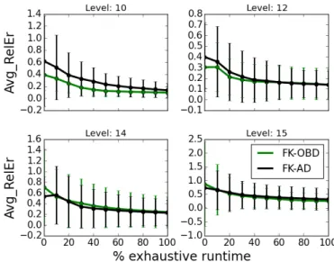
approach.. . . 52 3.7 An example of a pattern graph . . . 61 3.8 KLD averaged over all sampling iterations as a function of the

synthetic datasets . . . 65

(25)

3.9 Relative error averaged over all iterations of the sampling algorithms as a function of the synthetic datasets. . . 65 3.10 Relative error as a function of time averaged over patterns that

do not have an OBD for the DBLP dataset . . . 66 3.11 Average KLD represented in logarithmic scale as a function of

the pattern size . . . 67 3.12 Average relative error represented in logarithmic scale as a

function of the pattern size. . . 68 3.13 Average relative error plots for a subset of results for DBLP dataset 68 3.14 Average relative error plots for each pattern size for YEAST dataset 69 3.15 Average relative error for incomplete runs of the exhaustive

approach for the DBLP and YEAST datasets. . . 70

4.1 Hybrid dependency network induced by an HRDN . . . 80

5.1 Edit distance between the learned and the handcrafted model as the function of the number of training interpretations . . . 101 5.2 Edit distance between the learned and the handcrafted model

and the as a function of the increasing domain size. . . 101 5.3 The WPLL for each approach on the PKDD’99 financial data set

as a function of the number of bins used for discretization . . . 107 5.4 The run time of each approach on the PKDD’99 financial data

set as a function of the number of bins used for discretization . 107

6.1 A simplified snapshot of relational regression tree for predicting the next x position of an object . . . 117 6.2 MICO arm performing a left tap action on the object in its vicinity125 6.3 Prediction of tap action with two objects. 1000 samples are shown

(26)

Introduction

1

"To start, press any key... Where’s the "Any" key?" Homer Simpson

Real-world applications such as robotics, medicine, molecular biology, and social networks, amongst others, exhibit complex relational structure comprising of generic entities. Each entity is described by a number of attributes, and is related to a number of other entities of the same or different type. These relationships are general patterns or templates that match specific instantiations of objects (e.g., all humans are mortal, so is Socrates), and can be represented with first-order logic. Moreover, the world in which objects interact might be uncertain, which necessitates the tools of probability. For example, in Goodreads, a social network for book lovers, people are entities that have discrete attributes (e.g., favorite book type) and numeric attributes (e.g., the average number of books they read per year), and are connected through friendship relations. There also exists uncertainty about the existence and nature of these relations (e.g., there is a 20% chance that people lie about having read a classic or a book that was read by most of their friends). Additionally, the environment where objects reside can exhibit

(27)

sequential changes or dynamics: the number of objects changes, relationships between objects appear and disappear, and the properties of objects evolve as they interact. For example, a user of Goodreads can be influenced by the aggregated opinion of some friends about a book, causing her to change her rating for the book.

Statistical relational learning (SRL) (Getoor and Taskar2007; De Raedt, Frasconi, et al.2008; De Raedt2008; De Raedt and Kersting2011), a subfield of machine learning, is concerned with developing formalisms that deal with structured and uncertain domains. The SRL formalisms compactly represent the structure of a domain in the form of regularities or patterns that are quantified by a set of parameters. The parameters of a pattern in SRL are shared or tied across different instantiations of the pattern, which enables compact representation.

There are several tasks in SRL. The most general and complex task is to learn the structure that captures the regularities in the domain. The task of parameter estimation is used to extract the parameters that quantify the regularities. This two tasks are coupled in that that we want learn the parametrized regularities that best explain the data. Given or learned parametrized models can be used to perform inference or answer queries about specific entity instantiations, possibly given some observation or evidence. The approaches in SRL mostly focus on modelling the static aspect of the relational data meaning that the data is seen as a snapshot consisting of all the objects and relationships between them at a specific point in time. However, many domains such as robotics have a temporal or dynamic aspect. Planning approaches for dynamic relational domains devise a sequence of actions based on the state transition model that quantitatively regulates how the attributes and relationships between objects transition from one state to another.

Despite its progress, many challenges exist in statistical relational learning. One important challenge is to design scalable and efficient learning algorithms. The inefficiency is related to the choice of the representation and time-consuming structure learning subroutines such as parameter estimation and inference. For example, if one does not care about strictly accurate representations, the structure learning could be made efficient by decomposing the process into learning smaller models independently. Also, subroutines such as parameter estimation can be performed faster by resorting to approximations.

A second challenge lies in the fact that besides exhibiting complex structure, uncertainty and dynamics, real-world domains are also hybrid, meaning that

(28)

THESIS STATEMENT 3

they contain both discrete and continuous variables. The usual approach is to discretize continuous variables prior to modelling, learning or inference, which imposes limits on the representation power and leads to a loss of information. This problem raises an interesting question on how to upgrade existing SRL formalisms to hybrid domains, and how to learn and query the hybrid models. A third challenge is to model and learn dynamics in hybrid domains. The challenge lies in learning expressive models that can capture how complex relationships between objects change over time. The learned model can be further used to perform planning. Moreover, the algorithms designed to model and plan in dynamic relational domains are usually evaluated on simulated data. Thus, the challenge would be to perform structure learning and planning with real robots acting in dynamic relational environments.

1.1 Thesis Statement

The goal of this thesis is to push the boundaries of SRL across three dimensions: scalability, expressivity and dynamics. Accordingly, we test the following claims. First, we hypothesize that adapting techniques for approximately counting the number of pattern embeddings in a graph can be adapted to perform scalable and accurate parameter estimation in SRL. Second, the increased expressivity of hybrid SRL formalisms can provide more accurate and scalable structure learning performance than when discretizing the domain prior to learning. And finally, learning dynamic relational models in hybrid domains described with relational features and features expressing the arithmetics between low-level attributes, can result in expressive models that contribute to good planning performance.

1.2 Contributions

This dissertation addresses the thesis statement by:

1. developing an approximate graph pattern counting approach by extend-ing the algorithm of Fürer and Kasiviswanathan (2008),

2. proposing the hybrid relational dependency networks (HRDNs) as a formalism to model both continuous and discrete variables in relational domains,

(29)

3. designing a learner of local models (LLM) to learn the structure of HRDNs, 4. extending LLM to work in dynamic environments.

Several common ideas are interwoven through these topics: extracting and modelling knowledge from rich relational domains, addressing some of the current open questions in SRL, and fusion of different formalisms and applications (e.g., combining graph-based representations with parameter estimation in SRL, using SRL for real-world robotics applications). Next, we present in more detail the contributions for each of the topics addressed in this thesis.

1. Our first contribution is to propose a new approach for approximately counting how many times a pattern occurs in a graph. This approach is based on a fully polynomial randomized approximation scheme suggested by Fürer and Kasiviswanathan (2008) for larger unlabeled undirected graphs. As relations of objects and their properties can be represented with graphs, we evaluate this approach on the task of parameter estimation for SRL. This contribution also comprises:

• Two algorithms for efficiently obtaining an ordered bipartite decomposi-tion (OBD) for an input pattern, which is necessary for the theoretical guarantees of the proposed approach to hold.

• A demonstration of how the count of pattern occurences in a graph can be used to collect the sufficient statistics needed for parameter estimation in SRL.

• An extensive experimental comparison of the proposed algorithm and two baseline algorithms on the application of parameter estimation in logical Bayesian networks (LBNs) (Fierens, Blockeel, Bruynooghe, et al.2005), an SRL formalism also used in (Ravkic et al. 2012).

• An experimental assessment of the approach on power law graphs, as opposed to the original theoretical work that only considered random graphs.

• An analysis of the influence of the input pattern and data graph prop-erties on the performance of the proposed and baseline approaches. • Two empirical demonstrations showing that the proposed approach: a) converges fast even for large patterns for which exact search fails to

(30)

CONTRIBUTIONS 5

finish in a given time, b) exhibits good performance even for patterns not covered by the theoretical guarantees of the approach.

Using LBNs as an SRL formalism to perform parameter estimation via graph sampling is just an arbitrary choice and other SRL formalisms can be used as well. In essence, the idea behind this approach is simple: the relationships between objects can be represented as graphs and approximately counting graph embeddings in larger datasets can be used to efficiently collect the sufficient statistics.

2. Our second main contribution are hybrid relational dependency works (HRDNs), a formalism that upgrades relational dependency net-works (RDNs) (Neville and D. Jensen2007), to hybrid domains. Relational dependency networks are a template language for creating propositional dependency networks (Heckerman et al.2001) that approximate a joint probability distribution over a set of variables. This contribution includes: • The syntax and semantics of hybrid relational dependency networks. • A demonstration of local models that can be used for representing the conditional probability distributions that parametrize hybrid dependencies.

• A discussion of approximate inference for HRDNs.

3. Our third contribution is to propose the novel learner of local models (LLM) structure learning algorithm for hybrid relational dependency networks. Since we upgrade relational dependency networks, we inherit their efficient structure learning method that optimizes the conditional probability distribution for each variable independently. This contribution also includes:

• A discussion on parameter estimation and scoring strategies. • An experimental comparison of our approach applied to both hybrid

and discretized domains to Markov logic networks (Domingos and Richardson2004), an SRL approach for modelling discrete data. • An empirical demonstration that learning directly in hybrid domains

instead of discretizing them prior to learning results in better models. 4. The fourth and final main contribution presented in this dissertation is the algorithm to learn the structure and the parameters of dynamic distributional clause (DDC) program representing a hybrid relational Markov

(31)

decision process. In order to realize this, we learn HRDNs (Ravkic et al. 2015) as a proxy to obtain DDCs. Even though this contribution relies on the formalism of HRDNs, in order to meet the needs for handling dynamic hybrid relational models we perform the following upgrades:

• The models are parametrized with relational regression trees. In the initial representation of HRDNs, the models were parametrized with conditional probability tables.

• We introduce relational features that are able to represent arithmetic operations between low-level features. We refer to them as equational features.

We then provide the following principal components of this contribution: • The DDC Tree Learner, an algorithm for learning DDCs in hybrid

domains.

• A real-world robotics experiment with a robot arm executing differ-ent tasks on a number of objects, which represdiffer-ents an interesting application for SRL.

• A real-world evaluation of the learned state transition model by using HYPE (Nitti, Belle, et al.2015), an existing planning algorithm for hybrid dynamic relational domains.

• A demonstration that the models learned with our approach generalize to unseen cases and that they can grasp interesting relations between objects, which are crucial for accurate prediction and planning.

1.3 Thesis Structure

This work is positioned in the field of statistical relational learning, which is concerned with relational, uncertain and, possibly, dynamic and hybrid domains. In Chapter2we provide necessary background for the components of SRL: probability distributions, modelling propositional data, modelling of relational data, modelling of statistical relational models, and finally modelling dynamic relational data. For illustrating the attribute-value data format, often used in machine learning, we used the real-world data and models obtained in the kinesiology study we did in:

(32)

THESIS STRUCTURE 7

Irma Ravkic, Benjamin Wittevrongel, Wannes Meert, Jesse Davis, Tim Aderik Gerbrands, Benedicte Vanwanseele “Predicting gait retraining strategies for knee osteoarthritis”. Workshop paper at ECML-PKDD conference, September 2015, Porto, Portugal

The next four chapters represent the technical core of this thesis and embody our four main contributions. In Chapter3we introduce and experimentally evaluate the proposed algorithm for approximately counting pattern embeddings in graphs, based on the theoretical work of Fürer and Kasiwiswanathan, which is then showcased on the task of parameter estimation for SRL. This chapter draws upon the following submission, which is under revision:

Irma Ravkic, Martin Znidarsic, Jan Ramon, Jesse Davis (2016) “Graph sampling for efficient parameter estimation in statistical relational learning”. ( under the revision at ECML-PKDD Data mining and Knowledge discovery journal)

Chapter4introduces hybrid relational dependency networks (HRDNs), our proposed upgrade of relational dependency networks to hybrid domains. In Chapter5we introduce the learner of local models (LLM), algorithm for learning the structure of HRDNs. Chapters 4 and 5 are based on the following published work:

Irma Ravkic, Jan Ramon, Jesse Davis (2015) “Learning relational dependency networks in hybrid domains”. In: Machine Learning Journal 2015, volume 100, pp. 217 - 254

In Chapter6we introduce an approach for learning dynamic hybrid relational models and then using the learned models for planning in a real-world robotics application. The work in this chapter is published as:

Davide Nitti*, Irma Ravkic*, Jesse Davis, Luc De Raedt (2016) “Learning the structure of dynamic hybrid relational models”. In Proceedings of the 22nd European Conference on Artificial Intelligence (ECAI) 2016, Volume 285, pp.1283-1290

(* The contributions of this work are equally shared by the authors.)

Finally, in Chapter7we summarize our work, provide the main conclusions and give possible directions for future work.

(33)

(34)

Background

2

"I don’t tell you how to tell me what to do, so don’t tell me how to do what you tell me to do." Bender (Futurama)

The previous chapter positioned our work within the field of statistical relational learning and gave a detailed introduction to our contributions. This chapter lays the foundations needed to present these contributions.

SRL combines two components to model complex domains. One component is the probability distribution for which we give the foundations in Section2.1. The second component upgrades the propositional representations, which we discuss in Section2.2, with the notion of related object classes. This upgrade to relational domains can be accomplished by using relational databases or first-order logic presented in Section2.3. After introducing these two components of SRL, we combine them together in Section2.4by presenting how to model statistical relational models. For the purpose of this dissertation we focus on how to model and upgrade dependency networks, a propositional graphical model, to relational dependency networks by using a (restricted) first-order logic. We finalize this chapter by providing the background on dynamic relational hybrid models and

(35)

planning in Section2.5. This involves a brief introduction to Markov decision processes (MDPs) and distributional clauses (DCs).

2.1 Probability Distributions

In this section we provide a short introduction to the probability theory notions used throughout this dissertation. A more in depth introduction can be found in Neapolitan (2003).

A random variable is a variable that can take on a set of possible values, each of which is associated with a specific probability or density. For example, when throwing a die, each of the six values of the die occurs with the probability of 1/6. We denote random variables with capital letter (e.g., X). The value or state of a random variable is denoted with a lower case letters (e.g., x). Each random variable has an associated range of values it can take denoted with range(X). The probability that a variable X takes a value x∈range(X)is denoted with P(X=x). We denote sets of random variables by boldface capital letters (e.g.,

X). The Cartesian product of the ranges of all variables in X represents a sample

space denoted as Ω and represents joint assignments to the variables in X. A particular instance of Ω is denoted by boldface lower case letters (e.g., x). Depending on the range, random variables can be discrete or continuous. A discrete random variable takes values in a countable set. For example, a die represents a discrete random variable which when tossed can show one of its six possible values. In contrast, a continuous random variable has an infinite number of possible values. For example, room temperature can be a continuous variable taking on real values (e.g., 37.1◦).

The probability that a random variable X will take a value xiand that another random variable Y will take a value yiis called the joint probability of X=xi

and Y=yiand is denoted as P(X=xi, Y=yi). Next we define a joint probability distribution over a set of discrete variables, and joint probability density over a set of continuous variables.

Definition 1. (Joint probability distribution) Given a set of discrete random

variables X, and the set of all assignmentsΩ to the variables in X, a joint probability distribution P(x)is a function that maps each assignment x ∈ Ω to a real number

(36)

PROBABILITY DISTRIBUTIONS 11 such that: ∀x∈Ω : 0≤P(x) ≤1 and

∑

x∈Ω P(x) =1

Definition 2. (Joint probability density) Given a set of continuous random

variables X, and the set of all the assignmentsΩ to the variables in X, a joint probability density p(x)is a function that maps each assignment x∈ Ω to a real number such that:

∀x∈Ω : p(x) ≥0 and

Z +∞

−∞ p(x)dx=1

If two random variables X and Y are independent their joint probability distribution is expressed as P(X, Y) =P(X) ·P(Y).

Definition 3. (Conditional probability distribution) Given a joint probability

distribution P(X, Y), the conditional probability distribution of X given Y is defined as

P(X|Y) = P(X, Y)

P(Y)

and is undefined if P(Y) =0.

A similar definition holds for a conditional density function. The difference is that P(X, Y)and P(Y)are replaced with densities denoted p(X, Y)and p(Y), respectively.

Conditional dependencies play a crucial role in probabilistic reasoning systems. First, instead of being interested in the joint probability of events, in real life we are mostly interested in obtaining the probability of an event conditioned on some other event serving as evidence. Second, as we will see in the following section when we introduce probabilistic graphical models, the conditional

(37)

probabilities are used to factor joint probability distributions leading to efficient representations.

2.2 Modelling Propositional Data

Since its beginning, machine learning approaches have focused on so-called propositional or attribute-value representations (Mitchell1997). There are many approaches in machine learning that operate on this format of data, such as decision tree induction (Quinlan1986), rule induction (Clark and Boswell1991), and artificial neural networks, amongst others. In this section we illustrate these representations, and we introduce probabilistic graphical models (PGMs) (Koller and Friedman2009) as powerful tools for representing propositional data. In this dissertation we rely on dependency networks (DNs) (Heckerman et al.2001), a PGM that offers an efficient learning strategy.

2.2.1 Single-Table Representation

In many machine learning applications it is natural to assume that data comes in a single table with the attribute-value format where each row represents an example or an instance and columns represent attributes of those instances.

Example 1. Consider a kinesiology scenario (Ravkic, Wittevrongel, et al.2015) of tracking a number of healthy patients running with a number of sensors positioned on their body for the purpose of recording the data characterizing their habitual gait. Each patient is then labeled by an expert with a gait retraining strategy that best reduced knee osteoarthritis. The instructions for the patients are to either lean right with the torso (Trunk Lean) or to move the right knee inwards/medial (Medial Thrust). The natural choice for representing this data is the single-table format where each row represents one patient and each column represents attributes describing the patients’ habitual gait. A small example of this data is provided in Table2.1. The task would be to predict the best retraining strategy for a patient given her gait attributes.

The attribute-value data format is also called propositional because each row or example in the single-table format can be described with a fixed-size set of Boolean attributes or propositions. Propositions are atomic formulas of propositional logic and can be true or false. An interpretation is a function that assigns truth values to the propositions, and each example is one interpretation.

(38)

MODELLING PROPOSITIONAL DATA 13

Patient name Tibia angle Trunk angle Knee abduction ... Best strategy

Pete 5.5 3.9 7.0 ... Medial Thrust

Ann 6.3 -1.6 1.5 ... Trunk Lean

Mary 6.7 5.6 -2.4 ... Trunk Lean

. . .

Table 2.1: An illustration of an attribute-value format that in a single table captures a scenario from kinesiology experiment to predict the best gait retraining strategy (Best strategy) given a number of attributes of patients’ casual gait.

Usually a closed-world assumption (CWA) is made meaning that the values of the attributes that are not specified in the data are considered to be false.

Example 2. The first instance or row in Table2.1can be represented as an ordered set of the following propositions {Patient name=Pete, Tibia angle = 5.5, Trunk angle = 3.9, Knee abduction = 7.0, . . . , Best Strategy_=Medial Thrust}. Under CWA all other propositions for this example, such as Tibia angle=2.5, are false.

Decision Trees

One can apply a number of predictive or descriptive propositional machine learning approaches to the single-table attribute-value format of the data. The predictive approaches aim at learning the model that is good at predicting a target attribute on unseen data. Descriptive approaches on the other hand do not consider any attribute to be the target but they aim at describing the data or finding general regularities in the data. In this dissertation we use a mixed approach: we aim at extracting general regularities from the data, but underneath we use predictive models to accomplish this.

A widely used predictive model in machine learning are decision trees (Quinlan 1986) consisting of internal nodes which represent tests performed on attributes, and leaf-nodes which decide the label of an instance. Decision trees classify instances by sorting them from the root of the tree to a leaf-node reached by following the path established by successful internal node tests. A decision tree that was learned on the full kinesiology data is shown in Figure2.1. It can be seen that two attributes are selected by the decision tree learning algorithm to

(39)

be the internal tests. As these are numeric attributes, they are discretized and each branch leads to a specific prediction for the best gait retraining strategy. There are different tasks in predictive learning depending on whether the target attribute is discrete or continuous. For predicting discrete target attributes one uses classification, and for predicting a continuous target attribute one uses regression. Consequently, in case the class attribute is continuous the tree is a regression tree such that the leaves contain numbers. In other cases we wish to build a decision tree that would be used to estimate the probability distribution over the target attribute given other attributes. The leaves of this kind of regression tree would contain probability distributions which makes them probability trees. For example, in the tree in Figure2.1the leaves would contain a probability distribution over Best strategy values. One branch might state that the probability distribution is[0.2, 0.8]for values[Medial Thrust, Trunk Lean] given that−11.5<Knee abduction< −6.0.

Figure 2.1: A decision tree learned from the dataset in Table2.1.

Popular descriptive approaches in machine learning are probabilistic graphical models, and we introduce them in more detail in the following section.

2.2.2 Probabilistic Graphical Models

Probabilistic graphical models (PGM) (Koller and Friedman2009) are a marriage between probability theory and graph theory. They represent a neat framework for compactly representing joint probability distributions with simpler factors obtained by exploiting the conditional independencies between random

(40)

variables. The need for this modularity comes from the fact that the number of parameters needed to encode a joint probability distribution is exponential in the number of random variables. For example, for n binary random variables we would need 2n−1 independent parameters to parametrize the joint probability distribution (the nth is determined from others since probabilities need to sum to one). The most popular PGMs are Bayesian (Pearl1988) and Markov (Bishop 2006) networks. We will provide a very short introduction to them, because they are not the main focus of this dissertation. However, we will examine dependency networks(DNs) (Heckerman et al.2001) in more detail, which is a PGM that serves as one of the foundations for this dissertation.

Bayesian Networks

Given a set of random variables, a Bayesian network (Pearl1988) is a directed acyclic graph G = (V, E) where the nodes V represent a set of random variables X and the edges represent direct dependencies between the random variables. A Bayesian network graph is parameterized with a set of conditional probability distributions (CPDs) for each Xi ∈X given its parents in the graph,

P(Xi| Parents(Xi)). A probability of a specific value assignments to Xiand Parents(Xi)is denoted P(Xi =xi| parents(Xi)).

(a) (b) (c) (d)

Figure 2.2: Examples of simple dependency graphs that represent a) the Bayesian network encoding P(X, Y) =P(X)P(Y|X), b) the Bayesian network encoding P(X, Y) = P(Y)P(X|Y), c) the undirected graph representing the Markov network, d) the bidirectional dependency graph with P(X|Y)and P(Y|X)conditional distributions.

The structure of a Bayesian network entails some conditional independencies: each variable is conditionally independent of all its non-descendants in the graph given the value of all its parents. This property enables a factorization of the joint probability distribution over X in the following way. Given G together with

(41)

CPDs for each random variable, the joint probability for a set of assignments x for X is calculated as:

P(x) =

N

∏

i=1

P(Xi=xi|parents(Xi)) (2.1)

Examples of the simplest Bayesian networks are graphs in Figure2.2aand Figure2.2band the joint probability distribution encoded by these graphs are P(X, Y) =P(X)P(Y|X)and P(X, Y) =P(Y)P(X|Y), respectively.

Example 3. Consider the Bayesian network in Figure2.2aand the following parameters if we assume that X and Y are Boolean variables: P(X = True) = 0.2, P(Y =

True|X = True) = 0.5, and P(Y = True|X = False) = 0.2. Note that we can extract the parameters of other assignments by using the rule of probability theory stating that given a specific condition the probabilities of an event and its negation should sum up to 1. Hence, it holds that P(X= False) =1−P(X = True), and P(Y=False|X=True) =1−P(Y=True|X=True), etc. The joint probability distribution of this network is shown in Table2.2and it can be seen that the joint probabilities over all the assignments (the joint probability distribution) sum to 1. That is, we say that the Bayesian network encodes the proper joint probability distribution over its variables.

X Y P(X, Y) =P(X) ·P(Y|X)

True True 0.2·0.5=0.10 True False 0.2·0.5=0.10 False True 0.8·0.2=0.16 False False 0.8·0.8=0.64

Table 2.2: The joint probability distribution for the Bayesian network in Figure2.2aand parameters given in Example3.

Markov Networks

A Markov network (Bishop2006) uses an undirected graph G= (V, E)where the nodes in V represent a set of random variables X and the edges in E correspond to probabilistic interaction or correlation between neighboring random variables. The Markov network is parametrized by a set of potential functionsΦ. These potential functions are defined over cliques which represent

(42)

complete subgraphs of G. Let C be a set of cliques of a Markov network G. Each clique c∈C consists of a set of nodes Xcand is associated with a clique potential φc(xc)which is a non-negative function over the possible assignments to xc. Given a Markov network graph G and a set of potential functions Φ, the joint probability over random variables of G is expressed as:

P(x) = 1

Z_c∈C

∏

φc(xc) (2.2) where Z =∑X∏c∈Cφc(xc)is the normalizing constant, which ensures that P(X) is a proper joint probability distribution. Note that for the joint probability distribution of Bayesian networks in Equation2.1it holds that Z=1 since the acyclicity property ensures the proper joint probability distribution.

Example 4. A simple example of a Markov network with one clique over X and Y

variable is shown in Figure2.2c. Let the factors of this network be: φc(X=True, Y=

True) = φc(X = False, Y = False) = 0.6 and φc(X = True, Y = False) =

φc(X=False, Y=True) =0.4. It holds for this example that Z=2. To obtain the

joint probability, each factor needs to be normalized. For example, P(X=True, Y=

True) =0.6/2=0.3. This indeed ensures that the probability distribution sums to one:∑xP(x) =0.6/2+0.3/2+0.4/2+0.4/2=1.

Next we introduce dependency networks in more detail because they will serve as the basis for the work we do in this dissertation.

Dependency Networks

Unlike Bayesian networks and Markov networks, dependency networks (DNs) (Heckerman et al.2001) approximate a joint probability distribution over a set of random variables with a set of conditional probability distributions (CPDs) learned independently. A DN can be represented visually as a directed graph G = (V, E), containing one vertex VX for each randvar X ∈ X and a directed arc from vertex VX to vertex VYiff X ∈ Parents(Y). Each randvar X∈X has an associated conditional probability distribution P(X|Parents(X)), where Parents(X) ⊆X\ {X}.

Example 5. A simple example of a dependency network is shown in Figure2.2d. Note that the edge between X and Y is bidirectional. There are two CPDs quantifying the dependencies in this example: P(X|Y)and P(Y|X).

(43)

A dependency network is said to be consistent if there exists a probability distribution P that is consistent with the conditional distributions of the DN. This means that each of the CPDs can be extracted from the joint distribution by applying the rules of probability. If there is no such probability distribution, the DN is called a general dependency network and in the remainder of the text we will use the term dependency networks when we think of general DNs. Moreover, the product of CPDs in a general dependency network does not give the joint probability of variables, but their pseudo-likelihood (Besag1974):

PL(x) =

N

∏

i=1

P(Xi =xi|parents(Xi)). (2.3)

This means that dependency networks do not impose that CPDs factor the joint probability distributions and calculating the normalization constant in Equation 2.2 is avoided. The reader interested in literature on compatible conditionals and consistent distributions should read the work of Arnold and Press (1989). Next, we illustrate the consistent and inconsistent DNs in Example6.

Example 6. Consider the following CPTs (Lowd2012) for the dependency network in Figure2.2d:

P(X=True|Y=True) =4/5 P(X=True|Y=False) =2/5 P(Y=True|X=True) =2/3 P(Y=True|X=False) =1/4

There exists a joint probability distribution

P(X=True, Y=True) =0.4 P(X=True, Y=False) =0.2 P(Y=True, X =True) =0.1 P(Y=True, X=False) =0.3

consistent with the CPDs above. The reader can check that for each assignment to values of X and Y it holds that P(X|Y) =P(X, Y)/P(Y)and P(Y|X) =P(X, Y)/P(X). Now consider the following DN:

P(X=True|Y=True) =4/5 P(X=True|Y=False) =1/5 P(Y=True|X=True) =1/5 P(Y=True|X=False) =4/5

(44)

The CPD for P(X|Y)encourages X and Y to be equal, while the CPD for P(Y|X)

encourages X to be Y different. Hence, this DN is inconsistent and there does not exist a joint distribution from which these CPDs can be extracted.

Parameter Learning. For a given dependency Xi |Parents(Xi)the CPD can be any probabilistic regression or classification model and its parameters are estimated by performing parameter estimation. Parameter estimation is based on the maximum likelihood method which finds the set of parameters that maximize the likelihood, i.e., probability of data given the model. The standard choices for modelling the CPDs are the following:

• Conditional probability table (CPT) for a dependency Xi|Parents(Xi)

provides the probability distributions over values of Xi given the instantiations to the variables in the parent set Parents(Xi). The max-imum likelihood estimation of the CPT parameters from data is quite straightforward. For each possible joint instantiation parents(Xi)to the variables in Parents(Xi)we provide probabilities for each value xiof Xi

by counting in the following way:

Pest(Xi=xi|parents(Xi)) =

Nx_i,parents(X_i)

Nparents(Xi)

(2.4)

where Nxi,parents(Xi)represents the number of data instances in which Xi= xiand Parents(Xi) =parents(xi). In order to avoid potential problems of extreme probability values of 0 one can use the Laplace correction:

Pest(Xi=xi|parents(Xi)) =

Nxi,parents(Xi)+1 Nparents(Xi)+ |range(Xi)|

(2.5)

where range(Xi)represents a set of values that variable Ximay attain, and|range(Xi)|represents its cardinality.

• Logistic regression gives the probability of a discrete random variable conditioned on a number of discrete or numeric predictors. More generally, if Xi can take on any of the discrete values {x1, . . . , xK}, then the probability for Xi=x1, Xi=x2, . . . , Xi=xK−1given the instantiation of

(45)

the parents, parents(Xi), is: P(Xi =xk|parents(Xi)) = exp(ωk0+∑y_i∈parents(Xi)ωkyiyi) 1+_∑K−1_j=1 exp(ωj0+∑y_i∈parents(Xi)ωjyiyi) (2.6) When Xi =xK, it is: P(Xi =xk|parents(Xi)) = 1 1+_∑K−1_j=1 exp(ωj0+∑yi∈parents(Xi)ωjyiyi) (2.7)

To avoid overfitting when training logistic regression the solution is to introduce regularization term which penalizes large values of the weights W that parametrize the logistic regression. The regularized approach to learning a logistic regression function is to choose the weights such that the conditional data likelihood is maximized:

W←arg max

W

∑

l

lnP(xl_i|parents(Xi)l, W) −λkWk (2.8)

which adds the penalty proportional to the squared magnitude of W and where xli and parents(Xi)lrepresented the values of the respective variables in the lth training example, and λ represents a constant that gives strength to the term.

• Probability trees consist of the internal nodes representing the binary tests, and leaves containing probability distributions for the target variable Xi. The probability in a leaf K is calculated as

K_xi,parents(_Xi)

Kparents(_Xi) , where

Kxi,parents(Xi)represents the number of data instances in the leaf K. The Laplace correction can also be applied in the same way as for CPTs. A problem with using CPTs as the representation for conditional probability distributions is their inefficiency for a larger number of parents: the number of independent parameters needed to encode a CPT grows exponentially with the number of parents. Probability trees offer a sparser representation of CPDs by capturing context-specific independence (Boutilier et al.1996).

Structure Learning. There are three aspects that need to be addressed when

(46)

structures. Second one needs to evaluate the “goodness” of different candidate structures. And finally, one needs to define an effective search procedure that finds a good structure. In this thesis we consider a fully observable case and we make a closed world assumption. When learning DNs one optimizes the logarithm of Equation 2.3 or the pseudo-loglikelihood (PLL). The PLL of an assignment x to randvars X of a DN is calculated as:

PLL(x) =

N

∑

i=1

log[P(Xi=xi|parents(Xi))]. (2.9)

Optimizing the PLL has the advantages that it can be decomposed into maximizing the loglikelihood for each variable independently and calculating it does not require computing the partition function (that is, summing over all possible configurations of the randvars). This has a significant impact on the computational efficiency of the search algorithm. Note that this learning procedure is not possible for Bayesian networks since it could lead to a cyclic structure which is not allowed. In other words, learning the structure of a DN from data requires determining Parents(X)for each X∈X (i.e., the dependency structure) and the parameters of the CPD for X that maximize PLL. For example, one can consider algorithms based on greedy hill-climbing search driven by the score metric: a current candidate structure is maintained and iteratively improved until the score does not increase (Getoor, Friedman, et al.2001). One issue with structure learning of probabilistic graphical models is overfitting: if we perform likelihood maximization, the most complex structures will always be favored. There are ways to avoid this problem. First, using the Bayesian approach (Heckerman1999) that uses a prior distribution over the parameters can smooth the irregularities in the training data. Second, one can add hard constraints by selecting a less expressive hypothesis class (e.g., limit the number of parents in the parent set). Third, a simpler model can be preferred which corresponds to the principle of Occam’s razor: introduce a penalty term that penalizes complex structures. One such adaptation of the scoring function is the minimum description length (MDL) principle (Schwarz1978), based on ideas from information theory, which leads to the best compression of the data. Finally, the objective function can be augmented with a regularization term.

Inference. Learning each CPD independently could result in an inconsistent

model. That is, there may be no joint probability distribution such that it is possible to apply the rules of probability to the joint distribution in order to

(47)

derive each learned CPD. Regardless of whether a DN is consistent, applying an ordered Gibbs sampler to the DN’s CPDs results in a unique distribution, given that each variable in the DN is discrete and each CPD in the DN is positive (Heckerman et al.2001). If the DN is consistent, then its conditional distributions must be consistent with a Markov network, and Gibbs sampling converges to the same distribution as that of the Markov network. In case of an inconsistent DN, the stationary distribution may depend on the order in which variables are sampled, and the joint distribution determined by the Gibbs samples may be inconsistent with the CPDs.

Ordered Gibbs sampling randomly selects the initial value for each random variable, and then in each Gibbs sweep iterates over the variables in a fixed order and resamples the value of each Xi from its local distribution P(Xi|Parents(Xi). If the DN is consistent, it generates the joint probability distribution. If the DN is inconsistent, this procedure is called an ordered pseudo-Gibbs sampler (Heckerman et al.2001).

2.3 Modelling Relational Data

A disadvantage of the attribute-value representation is that many real-world problems, such as ones in chemoinformatics (King et al.2001), are relational and it is often hard, too lossy and incomprehensible to force the data about a particular example into a single row. This approach is usable for simple domains such as presented in Table2.1. However, a more complex problem (e.g., the patients are related, a single patient has multiple observation sessions under different conditions and labs) cannot be represented by a single table. In this case one would need to use representations adequate for modelling relational domains.

2.3.1 Relational Data and Databases

A relational database is a database that consists of multiple related tables. Each table represents a relationship between classes of objects or their attributes. Each entry in a table is characterized with a unique identifier called the primary key. The connection between tables is accomplished by means of foreign keys: one or more columns in a table that are primary keys in some other table. The relationships between tables can be of several types. If one row in a

(48)

MODELLING RELATIONAL DATA 23

table corresponds to exactly one row in another table, we call it a one-to-one relationship. In case one row in a table corresponds to multiple rows in another table we call it a one-to-many relationship. Finally, the connection when multiple rows in one table correspond to multiple rows in another table is called a many-to-many relationship.

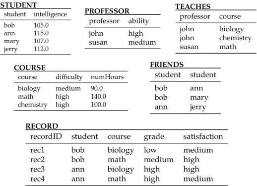
We will now introduce a toy example of a slightly modified university domain introduced by Getoor, Friedman, et al. (2001) that will be used as an example throughout the thesis.

Example 7. Consider a university consisting of students, professors and courses.

Students have an intelligence and can be friends with other students. A student can take a number of courses and express her satisfaction with each course she took and for which she got a grade. A course has a specific difficulty and a designated number of hours a student should spend on preparing it. Each course is taught by a professor who has a specific ability. A relational schema and a small number of examples is presented in Table2.3. The underlined columns represent primary keys, and bold column names denote foreign keys. Note that the foreign key in the RECORD table is a combination of the student and the course names. We can notice a couple of relationships between the tables. These relationships are accomplished through foreign keys. For example, the student column is the primary key in the STUDENT table, but a foreign key in the FRIENDS and the RECORD tables. TEACHES and RECORD are an example of a many-to-many connection: each professor can teach multiple courses, and a course can be taught by multiple professors; also each student can take multiple courses, and a course can be taken by multiple students.

Relational data can be processed in three different ways.

1. The first way is to flatten or propositionalize (Kramer et al. 2000) the relational data prior to its usage, and thus obtain the attribute-value format we illustrated in Section2.2.1. Advantages of this approach are its simplicity and the fact that there exists an abundance of propositional learning approaches. However, one disadvantage of this approach is that it produces propositional data with many attributes. This occurs due to the complicated relationships that might exist between objects, such as one-to-many and many-to-many relationships.

2. Instead of propositionalizing data prior to learning, features can be constructed while learning and constructed in such a way that they represent attributes of general object classes and relations between them.

(49)

STUDENT student intelligence bob 105.0 ann 115.0 mary 107.0 jerry 112.0 PROFESSOR professor ability john high susan medium TEACHES professor course john biology john chemistry susan math COURSE

course difficulty numHours biology medium 90.0 math high 140.0 chemistry high 100.0 FRIENDS student student bob ann bob mary ann jerry RECORD

recordID

student

course

grade

satisfaction

rec1

bob

biology

low

medium

rec2

bob

math

medium

high

rec3

ann

biology

high

rec4

ann

math

high

medium

Table 2.3: A simplified example of a relational database inspired by the university example described in Example7.

A tool that would enable this kind of modelling is first-order or predicate logic. A natural way to solve these tasks is the by using the inductive logic programming (ILP) approaches (Muggleton and De Raedt1994). ILP is a subfield of machine learning that addresses relational learning. In principle, ILP allows induction over relational structures which can make the learning intractable. Thus, different heuristics are used in ILP methods (Muggleton and De Raedt 1994) to control the search, and learn the concept efficiently. While there are a number of approaches for learning ILP programs, unless restrictions on the hypothesis space are made, the learning might be intractable, inflexible and inefficient in large scale domains.

3. Another option is the combination of relational learning with proposi-tional approaches (Roth and Yih2001; Davis, Burnside, Castro Dutra, et al. 2005; Landwehr, Kersting, and De Raedt2005; Landwehr, Kersting, and Raedt2007), which is the strategy we adopt in this thesis as well. The

(50)

MODELLING RELATIONAL DATA 25

general idea behind this approach is to encode relational structures as propositional representations in order to support flexible and efficient learning and evaluation, but to express the learned concepts in relational representations. While in ILP relational features are generated as a part of the structure search, in this method, the relational features are calculated up front.

2.3.2 Representations Based on First-Order Logic

Unlike propositional logic where we only have propositions that can be true or false, in first-order logic the notion of an object class is introduced, which together with quantification (existential and universal) represents an adequate tool (Lloyd2012) to compactly represent complex relational domains.

In this dissertation we use a variation of datalog, a type of restricted first-order logic. The alphabet of our language consists of three types of symbols: constants, logical variables, and predicates. A constant represents a specific object and is denoted with a lower-case letter (e.g., pete). A logical variable (logvar) X is a variable ranging over the objects in the domain. Logical variables may be typed in which case they represent placeholders for a specific subset of objects in the domain. Predicate symbols P/n, where n≥0 is the arity of the predicate, represent properties of objects or relations among objects. Each predicate P has a finite range, denoted range(P). In traditional logic, the range of a predicate is

{f alse, true}. However, in this thesis we allow a predicate to have a categorical or numeric range. For example, the range of a student’s intelligence could be

{low, med, high}or a range that is the interval of[0, 180]. An atom is of the form P(t1, . . . , tn)where P/n is a predicate and each tiis a constant or a logvar. In a typed language every argument position of an atom has a type. For example, in atom grade(S, C)we can constraint that logvar S ranges only over students and C only over the courses. The range of an atom is the range of its predicate. A literal is an atom or its negation. An atom is ground if all its arguments are constants. A substitution, denoted{X1/t1, . . . , Xn/tn}, maps each logvar Xito ti, where ti

is a logvar or a constant. A grounding substitution θ for an expression (e.g., an atom or a set of logvars) maps each logvar occurring in that expression to a constant. The set of all grounding substitutions for an expression E is denoted grsub(E). The result of applying a substitution to an atom a is denoted aθ.

Given a relational database, we can built a number of rules that define its content, but were not explicitly represented in the database. The rules in logic

Probabilistic Logical Models for Large-Scale Hybrid Domains

HAL Id: tel-01462085

https://hal.archives-ouvertes.fr/tel-01462085

Submitted on 18 Dec 2017

HAL is a multi-disciplinary open access

archive for the deposit and dissemination of

sci-entific research documents, whether they are

pub-lished or not. The documents may come from

teaching and research institutions in France or

abroad, or from public or private research centers.

L’archive ouverte pluridisciplinaire HAL, est

destinée au dépôt et à la diffusion de documents

scientifiques de niveau recherche, publiés ou non,

émanant des établissements d’enseignement et de

recherche français ou étrangers, des laboratoires

publics ou privés.

Domains

Irma Ravkic

To cite this version:

Irma Ravkic.

Probabilistic Logical Models for Large-Scale Hybrid Domains.

Machine Learning

[stat.ML]. KU Leuven, 2016. English. �tel-01462085�

ARENBERG DOCTORAL SCHOOL

Faculty of Engineering Science

Probabilistic Logical Models

for Large-Scale Hybrid

Domains

Irma Ravkic

Dissertation presented in partial

fulfillment of the requirements for the

degree of Doctor in Engineering

Science: Computer Science

October 2016

Supervisor:

Prof. dr. Jesse Davis

Probabilistic Logical Models for Large-Scale Hybrid

Domains

Irma RAVKIC

Abstract

Beknopte samenvatting

Acknowledgements

Contents

List of Symbols

List of Figures

Introduction

1

1.1 Thesis Statement

1.2 Contributions

1.3 Thesis Structure

Background

2

2.1 Probability Distributions

∑

2.2 Modelling Propositional Data

2.2.1

Single-Table Representation

2.2.2

Probabilistic Graphical Models

∏

∏

∏

∑

∑

2.3 Modelling Relational Data

2.3.1

Relational Data and Databases

recordID

student

course

grade

satisfaction

rec1

bob

biology

low

medium

rec2

bob

math