HAL Id: hal-01113938
https://hal.archives-ouvertes.fr/hal-01113938
Submitted on 6 Feb 2015
HAL is a multi-disciplinary open access
archive for the deposit and dissemination of
sci-entific research documents, whether they are
pub-lished or not. The documents may come from
teaching and research institutions in France or
abroad, or from public or private research centers.
L’archive ouverte pluridisciplinaire HAL, est
destinée au dépôt et à la diffusion de documents
scientifiques de niveau recherche, publiés ou non,
émanant des établissements d’enseignement et de
recherche français ou étrangers, des laboratoires
publics ou privés.
intensive and extensive biases
Rossana Mastrandrea, Squartini Tiziano, Giorgio Fagiolo, Diego Garlaschelli
To cite this version:
Rossana Mastrandrea, Squartini Tiziano, Giorgio Fagiolo, Diego Garlaschelli. Reconstructing the
world trade multiplex: the role of intensive and extensive biases. Physical Review E : Statistical,
Non-linear, and Soft Matter Physics, American Physical Society, 2014, 90 (6), pp.062804.
�10.1103/Phys-RevE.90.062804�. �hal-01113938�
the role of intensive and extensive biases
Rossana MastrandreaInstitute of Economics and LEM, Scuola Superiore Sant’Anna, 56127 Pisa (Italy)
and Aix Marseille Universit´e, Universit´e de Toulon,
CNRS, CPT, UMR 7332, 13288 Marseille (France) Tiziano Squartini
Instituut-Lorentz for Theoretical Physics, University of Leiden, 2333 CA Leiden (The Netherlands) and Institute for Complex Systems UOS Sapienza,
“Sapienza” University of Rome, P.le Aldo Moro 5, 00185 Rome (Italy) Giorgio Fagiolo
Institute of Economics and LEM, Scuola Superiore Sant’Anna, 56127 Pisa (Italy) Diego Garlaschelli
Instituut-Lorentz for Theoretical Physics, University of Leiden, 2333 CA Leiden (The Netherlands) (Dated: November 25, 2014)
In economic and financial networks, the strength of each node has always an important economic meaning, such as the size of supply and demand, import and export, or financial exposure. Con-structing null models of networks matching the observed strengths of all nodes is crucial in order to either detect interesting deviations of an empirical network from economically meaningful bench-marks or reconstruct the most likely structure of an economic network when the latter is unknown. However, several studies have proved that real economic networks and multiplexes are topologically very different from configurations inferred only from node strengths. Here we provide a detailed analysis of the World Trade Multiplex by comparing it to an enhanced null model that simultane-ously reproduces the strength and the degree of each node. We study several temporal snapshots and almost one hundred layers (commodity classes) of the multiplex and find that the observed properties are systematically well reproduced by our model. Our formalism allows us to introduce the (static) concept of extensive and intensive bias, defined as a measurable tendency of the network to prefer either the formation of extra links or the reinforcement of link weights, with respect to a reference case where only strengths are enforced. Our findings complement the existing economic literature on (dynamic) intensive and extensive trade margins. More in general, they show that real-world multiplexes can be strongly shaped by layer-specific local constraints.
I. INTRODUCTION
Over the last fifteen years, there has been a dramatic rise of interest towards the mechanisms of network for-mation [1, 2]. One of the reasons lies in the fact that the dynamics of a wide range of important phenomena (e.g. disease spreading and information diffusion) is strongly affected by the topology of the underlying network me-diating the interactions. Economic networks are partic-ularly relevant for the emergence of many processes of societal relevance such as globalization, economic inte-gration, and financial contagion [3].
In order to identify the non-trivial structural properties of a real network, one needs to appropriately define and implement a null model. Comparing a real network with a null model allows one to reveal statistically significant structural patterns. Substantial effort has been devoted to the definition of null models for graphs [4–12]. In eco-nomics, the use of purely random models is not new and spans from industrial agglomeration [13, 14] to interna-tional trade [15]. Identifying the observed properties of real economic networks carrying non-trivial information
allows one to select the ‘target quantities’ that economic models should aim at explaining or reproducing. In par-ticular, if a random network model where only a set of local node-specific properties are enforced turns out to reproduce a real-world network satisfactorily well, then there is no need to know additional information besides the chosen constraints. The latter are therefore max-imally informative, and the relevant (economic) models should aim at reproducing the observed values of the con-straints themselves. On the contrary, a bad agreement indicates the need for additional information.
An important economic case study is the World Trade Web (WTW) or International Trade Network (ITN), where nodes are world countries and links represent in-ternational trade relationships. At the aggregate level, various authors have focused on the binary version of the WTW [16–18], showing (among several other patterns) the presence of a ‘disassortative’ pattern and a stable negative correlation between node degree and clustering coefficient. The relevant role played by the topology on the whole network structure is undeniable. In fact, the observed properties turn out to be important in explain-ing macroeconomics dynamics. For instance, the degree
of a country has substantial implications for economic growth and a good potential for explaining episodes of financial contagion [19, 20].
The introduction of null models in the analysis of the WTW has allowed to (re)interpret the results of the net-work approach in the light of traditional economic analy-ses [21], where most country-specific macroeconomic vari-ables (total trade, number of trade partners, etc.) can be rephrased in terms of first-order (local) properties of nodes. Recent studies [22–24] have shown that much of the binary architecture of the WTW can be reproduced by a null model controlling for the (in- and out-) degrees of all countries. This null model is known as the Binary Configuration Model (BCM). The agreement between the BCM and the real WTW holds both at the aggregate level and at a ‘multiplex’ [25–28] level (i.e. for every dif-ferent commodity-specific layer of the network) [22, 23]. This result has important consequences for trade mod-elling, because it highlights the need for revised macroe-conomic theories aimed at reproducing the degrees of all countries, in contrast with the standard approach which considers the number of trade partners irrelevant.
Despite its fundamental role, the binary version of the WTW suffers from an important limitation: it ignores the magnitude of the observed trade relationships, thus giving only partial information about the network. In-deed, it turns out that the binary and weighted versions of the WTW are very different [29–31]. For example, the edge weight and node strength distributions are highly left-skewed, indicating that few intense trade connections co-exist with a majority of low-intensity ones [32] and that countries with many partners are also the richest and most (globally) central. However, the latter trade very intensively with only few of their partners (which turn out to be themselves very connected), forming few but intensive trade clusters (i.e. triangular patterns) [30]. Recent works [23, 33] have extended the binary null model analysis [22] to the weighted version of the WTW, now randomizing the latter while preserving each coun-try’s (in- and out-)strength. This null model is known as the Weighted Configuration Model (WCM). Surpris-ingly, these studies found a very bad agreement between observed and expected higher-order weighted properties, mainly because the randomized network is in general much denser than the observed one, and often almost fully connected. Other works obtained similar results us-ing different methodologies [11, 32, 34–36].
The standard interpretation of these findings calls for the existence of higher-order mechanisms shaping the structure of the WTW as a weighted network, suggesting the impossibility to reconstruct the WTW from purely country-specific information. Again, this interpretation has important consequences for economic modelling. In fact, reproducing the observed strengths or other purely weighted properties which, unlike the degrees, represent the main target of traditional macroeconomic theories (the most popular example being that of Gravity Mod-els [37–40]) appears quite useless in order to explain the
network structure. Even if for the opposite reason, this conclusion calls again for a change of perspective in the way economic models approach the international trade system. However, in this paper we show that this inter-pretation should be considerably revised.
There is another attractive reason for using null models in network analysis, namely the possibility of reconstruct-ing an (unobserved) network from its local properties. We recently introduced an enhanced method to build ensembles of networks simultaneously reproducing the strength and the degree of each node [41]. The method, called Enhanced Configuration Model (ECM) because it is an augmented version of both the BCM and the WCM, builds upon prior theoretical results introducing the gen-eralized Bose-Fermi distribution [42], which is the appro-priate probability function characterizing systems with both binary and non-binary constraints. The application of the ECM allowed us to show that, for many real net-works where the specification of the strengths alone give very poor results, the joint specification of strengths and degrees can reconstruct the original network to a great degree of accuracy [41].
While we already analysed one (aggregated and static) snapshot of the WTW as part of the analysis described above, this is not enough in order to conclude that those results can be straightforwardly extended to different temporal snapshots and different layers of this economic multiplex. Indeed, ref. [41] focused on a diverse set of networks of very different nature (biological, social, etc.), but included no temporal analysis and no multiplex anal-ysis. As we have already mentioned, in the particular case of the WTW carrying out a deeper analysis has a special importance for its macroeconomic implications, because understanding the empirical role of local con-straints changes the theoretical approaches to the trade system and can highlight some important flaws in stan-dard macroeconomic modeling. Previous investigations of the international trade network revealed similarities but also differences across the layers of the multiplex (at both binary and weighted levels) [43]. Moreover, in-creased product complexity appears to yield inin-creased product-specific network complexity [44]. Finally, the country-product associations reveal a highly nontriv-ial nested structure [45] which contradicts the main-stream economic expectation and, similarly, the product-product network displays a strong core-periphery struc-ture [46]. These product-related heterogeneities imply that it is not obvious whether one should expect that the results obtained on a single, aggregate instance of the WTW are robust over time and across different com-modity classes.
Given the importance of the problem and its more gen-eral implications for the understanding of economic net-works, in this paper we carry out an in-depth investiga-tion of the WTW spanning several years and different commodities. Our results show that, when considered together, the total trade (strength) and the number of trade partners (degree) of all world countries are enough
in order to reproduce many higher-order properties of the network, for all levels of disaggregation and all temporal snapshots in our analysis. In order to fully explain the structure of the WTW, binary constraints must there-fore be added to the weighted ones. Economically, this suggests that additional higher-order mechanisms besides those accounting for the joint evolution of degrees and strengths are not really necessary in order to explain the structure and dynamics of the WTW. On the other hand, we also show that degrees and strengths are ‘irreducible’ to each other, i.e. any minimal macroeconomic model aiming at reproducing the WTW should not discard any of the two quantities.
Our work complements the existing economic litera-ture about the so-called extensive and intensive margins of trade [47–49], defined as the preference for the network to evolve by establishing new connections or by strength-ening the intensity of existing ones respectively. While extensive and intensive margins are traditionally defined at an intrinsically dynamical level, we define the new con-cept of extensive and intensive biases as a purely static notion, and for each pair of countries separately. We fo-cus on cross-sectional data and evaluate whether, at a given point in time, pairs of countries are ‘shifted’ along the intensive or extensive direction as compared to an appropriate null model. Thus, our methodology does not establish whether the WTW proceeds along the extensive or intensive margin in the traditional ‘dynamical’ way, i.e. by accounting for the variation of trade connections and/or their weights over time. On the contrary, it allows us to identify a bias towards either the extensive or the intensive direction in a novel, static fashion, by exploit-ing a mathematical property of the null model specifyexploit-ing both strengths and degrees. Moreover, the entity of the bias can be exactly quantified for each pair of countries, allowing different pairs of nodes to be characterized by opposite tendencies.
Our paper is organized as follows. In Sec. II we in-troduce the trade data used and briefly summarize the methodology we employ to specify both strengths and de-grees in weighted networks [41, 50]. In Sec. III we apply the methodology first to a reference year, then to several temporal snapshots, and finally to different aggregation levels (commodity classes) of the world trade multiplex. In Sec. IV we discuss some general economic implications of our results and their relation with the more traditional literature about intensive and extensive margins of trade.
II. DATA AND METHODOLOGY
As we mentioned, our analysis builds upon previous studies of the WTW that showed that the degree se-quence is able to replicate the purely binary topology very well [22], while the strength sequence is completely
unable to replicate the weighted structure [33]. We
aim at understanding whether the joint specification of strengths and degrees allows us to successfully replicate
the weighted structure. To this end, we use exactly the same data set as refs. [22, 33], so that consistent com-parisons can be made. Such data set is described in sec. II A. We also use a similar, but appropriately generalized, methodology. This is introduced in sec. II B.
A. The world trade multiplex
As in refs. [22, 33], we employ international trade data provided by the United Nations Commodity Trade Database (UN COMTRADE [51]) in order to build a time sequence of binary and weighted trade multiplexes. The sample refers to 11 years (1992-2002) and the money unit is current U.S. dollars. The choice of this time span allows us construct a time-varying multiplex with a con-stant number of N = 162 countries and a concon-stant num-ber of C = 97 layers (commodity classes), evolving over T= 11 years. When necessary, we will also aggregate all or part of the layers to obtain different levels of resolu-tion.
We chose the classification of trade values into C = 97 possible commodities listed according to the Harmonized System 1996 (HS1996 [52]). For each year t (1 ≤ t ≤ T ) and each commodity c (1 ≤ c ≤ C), the starting data are represented as a matrix whose elements are the trade flows directed from each country to all other countries [53]. The matrix elements specifying the multiplex are denoted by e(c)ij (t), where e
(c)
ij (t) > 0 whenever there is an export of good c from country i to country j, and e(c)ij (t) = 0 otherwise. Rows and columns stand for ex-porting and imex-porting countries respectively. The value of e(c)ij (t) is in current U.S. dollars (USD) for all com-modities.
Given the commodity-specific (multiplex) data e(c)ij (t), we can compute the total (aggregate) value of exports eAGGij (t) from country i to country j summing up over the exports of all C = 97 commodity classes:
eAGGij (t) ≡ C X
c=1
e(c)ij (t) (1)
The particular aggregation procedure described above, introduced in [43], allows us to compare the analysis of the C commodity-specific layers of the multiplex with a (C + 1)-th aggregate network, avoiding possible incon-sistencies between the original aggregated and disaggre-gated trade data.
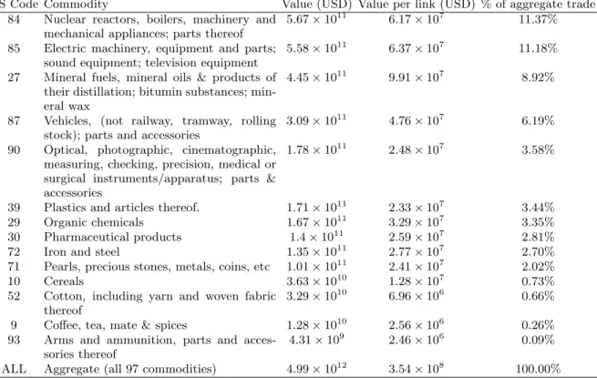
We put special emphasis on the 14 particularly rele-vant commodities identified in [43] and reported in ta-ble I. They include the 10 most traded commodities (c = 84, 85, 27, 87, 90, 39, 29, 30, 72, 71 according to the HS1996) in terms of total trade value (following the ranking in year 2003, [43]), plus 4 commodities (c = 10, 52, 9, 93 according to the HS1996) which are less traded but still important for their economic relevance. The 10 most traded commodities account for 56% of to-tal world trade in 2003; moreover, they also feature the
HS Code Commodity Value (USD) Value per link (USD) % of aggregate trade
84 Nuclear reactors, boilers, machinery and
mechanical appliances; parts thereof
5.67 × 10¹¹ 6.17 × 10⁷ 11.37%
85 Electric machinery, equipment and parts;
sound equipment; television equipment
5.58 × 10¹¹ 6.37 × 10⁷ 11.18%
27 Mineral fuels, mineral oils & products of
their distillation; bitumin substances; min-eral wax
4.45 × 10¹¹ 9.91 × 10⁷ 8.92%
87 Vehicles, (not railway, tramway, rolling
stock); parts and accessories
3.09 × 10¹¹ 4.76 × 10⁷ 6.19%
90 Optical, photographic, cinematographic,
measuring, checking, precision, medical or surgical instruments/apparatus; parts & accessories
1.78 × 10¹¹ 2.48 × 10⁷ 3.58%
39 Plastics and articles thereof. 1.71 × 10¹¹ 2.33 × 10⁷ 3.44%
29 Organic chemicals 1.67 × 10¹¹ 3.29 × 10⁷ 3.35%
30 Pharmaceutical products 1.4 × 10¹¹ 2.59 × 10⁷ 2.81%
72 Iron and steel 1.35 × 10¹¹ 2.77 × 10⁷ 2.70%
71 Pearls, precious stones, metals, coins, etc 1.01 × 10¹¹ 2.41 × 10⁷ 2.02%
10 Cereals 3.63 × 10¹⁰ 1.28 × 10⁷ 0.73%
52 Cotton, including yarn and woven fabric
thereof
3.29 × 10¹⁰ 6.96 × 10⁶ 0.66%
9 Coffee, tea, mate & spices 1.28 × 10¹⁰ 2.56 × 10⁶ 0.26%
93 Arms and ammunition, parts and
acces-sories thereof
4.31 × 10⁹ 2.46 × 10⁶ 0.09%
ALL Aggregate (all 97 commodities) 4.99 × 10¹² 3.54 × 10⁸ 100.00%
TABLE I. The 14 most relevant commodity classes (plus aggregate trade) in year 2003 and the corresponding total trade value (USD), trade value per link (USD), and share of world aggregate trade. From ref. [43].
largest values of trade value per link (see table I). Taken together, the 14 most relevant commodities account in total for 57% of world trade in 2003. As an intermedi-ate level of aggregation between individual commodities and fully aggregate trade, we also consider the network formed by the sum of the 14 special commodities. In this way we can also draw conclusions about the robust-ness of our methodology with respect to different levels of aggregation.
In our analyses, we will focus on the undirected (sym-metrized) representation of the network for obvious rea-sons of simplicity, even if the extension to the directed case is straightforward once the method in ref. [41] is ap-propriately generalized. In any case, several works have shown that the percentage of reciprocated interactions in the WTW is steadily high [22, 29, 33], giving us reason-able confidence that we can focus on the temporal series of undirected networks. We therefore define the symmet-ric matsymmet-rices ˜ wij(c)(t) ≡ $ e(c)ij (t) + e(c)ji (t) 2 ' , ˜ wAGGij (t) ≡ $ eAGG ij (t) + eAGGji (t) 2 ' (2) where bxe represents the nearest integer to the nonneg-ative real number x [54]. The above matrices define an undirected weighted network where the weight of a link
is the average of the trade flowing in either direction be-tween two countries.
In order to wash away trend effects and make the data comparable over time, we normalized our weights accord-ing to the total trade volume for each year:
wij(c)(t) ≡ w˜ (c) ij (t) ˜ wT OT(c) , wijAGG(t) ≡ w˜ AGG ij (t) ˜ wAGG T OT (3) where w˜(c)T OT = PN i=1 PN j=i+1w˜ (c) ij and w˜T OTAGG = PN i=1 PN j=i+1w˜ AGG
ij . In such a way, we end up with
adi-mensional weights that allow proper comparisons over time and consistent analyses of the evolution of network properties.
B. The Enhanced Configuration Model
Our methodology makes intense use of the ECM [41], defined as an ensemble of weighted networks with given strengths and degrees. In some sense, the ECM unifies the BCM and the WCM, which have been separately used in previous analyses of the same data [22, 33].
One can show [50, 55] that most of the algorithms de-veloped to randomize a real-world network suffer from severe limitations and give biased results. To overcome these limitations, we use a recently proposed unbiased method [41] based on the maximum-likelihood estima-tion [56] of maximum-entropy ensembles of graphs [50].
One of the attractive features of this method is its fully analytical character, which allows us to obtain the ex-act expressions for the expected values without perform-ing explicit averages over numerically sampled networks of the ensemble. Recently, a fast and unbiased algo-rithm has been released to computationally implement this procedure [55]. We briefly recall the main steps of this approach and of the enhanced network reconstruc-tion method that, building on some general theoretical results [42], can be derived from it.
Firstly, we need to specify a set of constraints {Ci}. The constraints are the network properties that we want to preserve during the randomization procedure, accord-ing to the specific network and research question. Gen-erally these constraints are local, such as the strength se-quence defining the WCM, but the methodology can also account for non-local constraints in some cases [57, 58]. In order to construct the ECM, defined an ensemble of weighted networks where both the degree sequence and the strength sequence are specified [41], we choose
{Ci} ≡ {ki, si} (4)
where ki stands for the i-th node degree and si for the i-th node strength.
Secondly, we need to find the analytical expression for the probability P (W ) that (under the chosen constraints) maximizes the Shannon-Gibbs entropy
S(W ) ≡ −X
W
P(W ) ln P (W ) (5)
over the ensemble of allowed networks. Note that P (W ) stands for the occurrence probability of the graph W in the ensemble of allowed weighted graphs, and the sums are over all such graphs. For our purposes, the allowed graphs are all the undirected networks with N vertices and non-negative integer edge weights. Each such net-work is uniquely specified by its N ×N symmetric weight matrix W , where the entry wij = wji∈ N represents the weight of the link connecting nodes i and j. The max-imization of Shannon’s entropy is done under the
con-straints P
WP(W ) = 1 (this ensures the normalization
of the probability) and hCii ≡PWP(W )Ci(W ) = Cifor all i (this fixes the desired structural properties). The for-mal solution [50] of this constrained maximization prob-lem can be written as
P(W |~θ) ≡ e −H(W,~θ) Z(~θ) , (6) where H(W, ~θ) ≡X i θiCi(W ) (7)
is the graph Hamiltonian and
Z(~θ) ≡X
W
e−H(W,~θ) (8)
is the partition function. The Hamiltonian is a linear combination of the constraints {Ci}, with the coefficients {θi} being the conjugate Lagrange multipliers introduced in the constrained-maximization problem.
For the ECM, it is possible to show [41, 42] that P(W |~x, ~y) =Y
i<j
qij(wij|~x, ~y), (9)
where ~x and ~y are two N -dimensional Lagrange multipli-ers (N stands for the number of nodes) controlling for the expected degrees and strengths respectively (with xi≥ 0 and 0 ≤ yi <1 for all i) and qij(w|~x, ~y) is the conditional probability to observe a link of weight w between nodes iand j. The latter has the explicit expression [41, 42]
qij(w|~x, ~y) =
(xixj)Θ(w)(yiyj)w(1 − yiyj) 1 − yiyj+ xixjyiyj
. (10)
The third step of the procedure prescribes to find the values of the Lagrange multipliers ~x∗, ~y∗ that maximize the log-likelihood of generating the observed weighted
network W∗ (which is one particular network in the
en-semble considered). The log-likelihood reads L(~x, ~y) ≡ ln P (W∗|~x, ~y) =X
i<j
ln qij(wij∗|~x, ~y) (11) representing the logarithm of the probability to observe
the empirical graph W∗. The maximization of the
like-lihood is equivalent to the requirement that the desired constraints are satisfied on average by the ensemble of networks [56], i.e. in this case hkii = ki(W∗) and hsii = si(W∗) for all i [41].
As a final step, one can use the Lagrange multipliers ~x∗, ~y∗ to compute the expected value hXi of any (higher-order) network property X(W ):
hXi ≡X
W
X(W )P (W |~x∗, ~y∗) (12)
Comparing hXi with the observed value X(W∗) allows
us to verify whether the ‘reconstructed’ value of the prop-erty is indeed close to the empirical one.
We will also compare the predictions of the ECM with those of the WCM. The latter can be obtained by setting ~x= ~1 and maximizing the likelihood with respect to ~y alone, thus finding another vector ~y∗∗6= ~y∗ [41].
A computationally fast and statistically unbiased al-gorithm to obtain the values of the Lagrange multipliers maximizing the likelihood of both the ECM and WCM (along with other maximum-entropy ensembles) has been recently introduced under the name of ‘Max & Sam’ (‘maximize and sample’) method [55]. We will use that algorithm in our analysis.
III. RESULTS
In this section, we first analyse in detail the aggregated trade network in the reference year 2002. Our choice of
this particular snapshot is dictated by the need to com-pare our results with that of refs. [22, 33], as we men-tioned. We then consider the temporal evolution of the system. Finally, we perform a multiplex analysis on the disaggregated, commodity-specific layers of the WTW.
A. Analysis of the aggregated network
For simplicity of the notation, in this subsection we indicate with A the adjacency matrix and with W the weighted matrix representing the aggregate network in year 2002, i.e. wij ≡ wAGGij (2002). In general, we can relate the entries of the matrices A and W through the
zeroth power using the notation w0
ij = aij, where we conventionally define 00≡ 0. This notation will be useful later to calculate the expected values of various structural properties. It also allows us to express the properties of purely topological properties, which in principle depend on the adjacency matrix A, as functions of the matrix W.
We are interested in assessing to what extent the ECM is able to replicate the higher-order properties character-izing the WTW over time. Therefore we first apply the ECM to the data, thus finding the vectors ~x∗ and ~y∗, and then we use these vectors to calculate the expected values of the chosen higher-order properties. For con-sistency with refs. [22, 33], we focus on the Average Nearest Neighbor Degree, the Average Nearest Neighbor
Strength (denoted by knn
i and snni respectively), the Bi-nary Clustering Coefficient and the Weighted Clustering Coefficient (denoted by ci and cwi respectively). In what follows, we first recall the analytical expressions of these higher-order quantities. Then, for the sake of clarity we write down the explicit expressions for the expected value of the same quantities under the ECM, i.e. the particular form taken by eq.(12) for each property under study.
The Average Nearest Neighbor Degree is defined as knni (W ) ≡ P j6=iw 0 ijkj ki = P j6=i P k6=jw 0 ijwjk0 P j6=iw0ij , (13)
where ki=Pj6=iw0ijstands for the i-th node degree, and represents the average of the degrees of the partners of node i, i.e. it provides a measure of the connectivity of the neighbours of that node.
The Binary Clustering Coefficient has the expression ci(W ) ≡ P j6=i P k6=i,jw 0 ijw0jkw 0 ki P j6=i P k6=i,jw 0 ijw0ki (14) and measures the tendency of node i to form triangles, i.e. it counts how many closed triangles are attached to node i, divided by the maximum number of triangles achievable by a node with degree ki.
The Average Nearest Neighbor Strength is defined as snni (W ) ≡ P j6=iw0ijsj ki = P j6=i P k6=jw0ijwjk P j6=iw 0 ij , (15)
where si = Pj6=iwij stands for the i-th node strength, and measures the average strength of the neighbors of vertex i. Similarly to its binary counterpart (knn
i ), snni reveals the ‘intensity’ of connectiviy of the neighbours of a node, now taking edge weights into account.
Finally, the Weighted Clustering Coefficient [59] can be defined as cwi(W ) = P j6=i P k6=i,j(wijwjkwki) 1/3 P j6=i P k6=i,jwij0wki0 (16) and measures the propensity of node i to be involved in triangular relations, taking into account the weights of such relations.
In order to compute the expected value of the above properties, it is necessary to compute the expected prod-uct of (powers of) distinct matrix entries. The indepen-dence of pairs of nodes in the ECM [41] ensures that
* X i6=j6=k,... wijα· wjkβ · . . . + = X i6=j6=k,... hwα iji · hw β jki · h. . . i.
Each individual term in the product is given by hwγiji = +∞ X w=0 wγqij(w|~x∗, ~y∗) = x∗ix∗j(1 − y∗ iyj∗)Li−γ(yi∗y∗j) 1 − y∗ iyj∗+ x∗ix∗jyi∗y∗j
where Lin(z) ≡ P+∞l=1 zl/ln is the nth polylogarithm of
z [41]. The simplest cases γ = 1 and γ = 0 yield the
expected weight hwiji ≡ x∗ix∗jyi∗yj∗ (1 − y∗ iy∗j)(1 − yi∗y∗j+ x∗ix∗jy∗iyj∗) (17) and the connection probability
pij≡ hw0iji = x∗ix∗jy∗iyj∗ 1 − y∗ iy∗j+ x∗ix∗jyi∗yj∗ (18) respectively [41].
As a result, the expected values of the purely topolog-ical (weight-independent) properties can be obtained by simply replacing w0 ij = aij with pij [41]: hknn i (W )i ≡ P j6=ipijhkji hkii = P j6=i P k6=jpijpjk P j6=ipij , (19) hci(W )i ≡ P j6=i P k6=i,jpijpjkpki P j6=i P k6=i,jpijpki (20) where, by construction, hkii ≡ ki for all i. For the ex-pected value of snn i we have [41, 42]: hsnn i (W )i ≡ P j6=ipijhsji hkii = P j6=i P k6=jpijhwjki P j6=ipij (21)
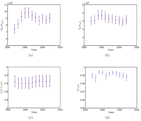
0 50 100 150 200 100 110 120 130 140 150 160 170 k k nn ,<k nn > 0 50 100 150 200 0.65 0.7 0.75 0.8 0.85 0.9 0.95 1 k c,<c> 102 104 106 108 1010 106 107 108 s s nn ,<s nn > 102 104 106 108 1010 100 102 104 106 108 s c w,<c w>
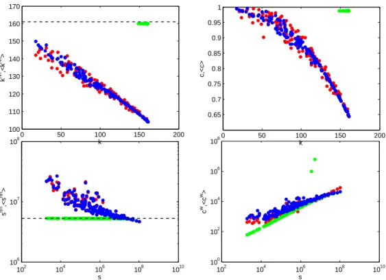
FIG. 1. Comparison between the observed undirected binary and weighted properties (red points) and the corresponding ensemble averages of the WCM (green points) and the ECM (blue points) for the aggregated WTW in the 2002 snapshot.
Top left: Average Nearest Neighbor Degree knn
i versus degree ki. Top right: Binary Clustering Coefficient ci versus degree
ki. Bottom left: Average Nearest Neighbor Strength snni versus strength si. Bottom right: Weighted Clustering Coefficient cwi
versus strength si.
where hsii ≡ si, ∀i. Finally, the expected value of cwi is hcw i (W )i = P j6=i P k6=i,jhw 1/3 ij ihw 1/3 jk ihw 1/3 ki i P j6=i P k6=i,jpijpki (22)
In fig. 1 we show, for the snapshot in year 2002,
the scatter plots between node degree (ki) and higher-order binary properties (knn
i , ci), as well as those between node strength (si) and higher-order weighted properties (snn
i , cwi ). From an economic point of view, kinn and ci give information about indirect interactions over paths of length 2 and 3 respectively, since terms of the form aijajk and aijajkaki are involved in the definitions of these quantities. In accordance with the existing litera-ture, we find decreasing trends of both knn
i and ci
ver-sus ki. This confirms that it is very likely to find nodes with many trade partners connected to nodes with small degree (disassortativity), while trade partners of poorly connected nodes are highly inter-connected. Similar con-siderations hold true when we consider edge weights, as snn
i and cwi involve indirect paths of length 2 and 3 respec-tively, now including mixed information about topology and weights. Intensively trading countries are found to be connected with poorly trading countries, confirming a dissasortative pattern (even if less prominent than in the binary case) at a weighted level.
Besides the observed values of the aforementioned quantities, in fig. 1 we also plot the corresponding ex-pected values predicted by the ECM, as well as those predicted by the WCM. The latter represent the start-ing point of our analysis, because they are intended to merely replicate the results in ref. [33]. Indeed, we con-firm that the WCM is in striking disagreement with the observed values. While, at a binary level, the empirical degree correlations and clustering structure of the ITN are excellently reproduced by the BCM (which uses only the knowledge of the degree sequence) [22], at a weighted level the observed network properties are very different from the predictions of the WCM (which, naively, is the obvious extension of the BCM to weighted graphs) [33]. These results are robust over time and for various reso-lutions (i.e., for different levels of aggregation of traded commodities).
It is important to realize the origin of the disagreement between the WCM and the real network. We note that the expected values under the WCM are similar to those predicted for a fully connected topology. Indeed, for a
complete network we have hkii = N − 1 (23) hknn i i = N − 1 (24) hci = 1 (25) hsnn i i = P isi N −1 = 2WT OT N −1 (26)
where N stands for the number of nodes in the network, while WT OT is the total weight of all edges. The above predictions can be confirmed in fig. 1. So, the main rea-son why the WCM fails is the fact that it generates unre-alistically dense (and sometimes almost fully connected) networks [33, 41]. We also note that, despite the apparent good agreement between the observed weighted cluster-ing coefficient and its expected value under the WCM (fig. 1), one can show that the empirical total level of clustering is in general higher than the one predicted by WCM, both throughout the temporal evolution of the system and across its commodity-specific layers [33].
We note that another study [36] also applied a variant of the WCM (basically assuming non-negative but real-valued, instead of integer-real-valued, edge weights) to the WTW. However, the quantities used therein to test the model against the data did not depend in any way on the adjacency matrix A, i.e. they were entirely topology-independent. As a result, the authors concluded that the observed WTW is a typical member of the WCM. Our analysis, together with ref. [33], shows that monitoring more (topological) properties leads to the opposite con-clusion. Indeed, it is easy to show that the variant of the WCM used in ref. [36] predicts a rigorously fully connected network, precisely because the assumption of real-valued weights implies a zero probability of missing links (zero weights). Therefore the real-valued WCM en-counters the limitations discussed above in an even more extreme way.
We now come to the predictions of the ECM shown in fig. 1. In marked contrast with the WCM, the ECM performs very well and reproduces both the binary and weighted properties of the WTW. Firstly, we find a
def-initely improved agreement for the binary trends (knn
i
and ci versus ki): the ECM shows an expected trend
that follows the data very closely. For these binary prop-erties, the predictions of the ECM are even closer to the observed cloud of points than the monotonic curves pre-dicted by the BCM for the same network, as a visual comparison with the results shown in ref. [22] immedi-ately reveals. Secondly, we also find a significantly better agreement, with respect to the WCM, between the
ob-served and the randomized weighted trends (snn
i and c
w i versus si).
These results imply that the knowledge of both the number of trade partners of each node and the total amount of trade flowing through each country is highly informative about the higher-order and non local dy-namics of the whole network. More in general, the lo-cal binary information is crucial in order to predict the
weighted structure itself. In turn, this means that the weighted information alone does not allow a deep under-standing of the topology of the network. We therefore confirm our recent finding [41] that the na¨ıve expectation that weighted quantities are per se more informative than the corresponding binary ones is fundamentally incorrect. To further validate these findings, in what follows we ex-plore the evolution of the same properties over time, and across different layers of the trade multiplex.
B. Temporal evolution
We first test the robustness of our results over time, by replicating the previous analysis on the 11 yearly snap-shots of the aggregated network. We measure the same properties, as well as their expected values, as defined
in sec. III A, where now the matrices A and W
re-fer to each of the various snapshots of the system, i.e. wij ≡ wijAGG(t) for t = 1992, 1993, . . . 2002.
We show our results in the following, more compact way. We consider the four network properties defined in eqs. (13)-(16) separately, and for each network property we take the list of observed values (e.g. {knn
i }) and the
list of expected values under the ECM (e.g. {hknn
i i}). For each of the two lists, we compute the following three metrics: i) the average value of the list; ii) the standard deviation of the list; iii) the Pearson correlation coeffi-cient between the list and the list of ‘natural’ constraints that we used above as the independent variable in the relevant scatter plot (e.g. {ki}). As a fourth metric, we also calculate: iv) the Pearson correlation coefficient be-tween the list of expected values and the list of observed values (e.g. between {knn
i } and {hk
nn
i i}). Each of these
four metrics summarizes one aspect of the scatter plot (of the type shown in fig. 1) for the structural property under consideration, thereby allowing us to compactly track the evolution of the system over time.
It should be noted that the use of the correlation co-efficient (iv ) is more appropriate than that of the coeffi-cient (iii ), since a perfect agreement between model and data implies an equality between expected and observed properties. Such an equality is a proper form of linear correlation, for which we expect the Pearson correlation coefficient to achieve its maximum value 1. In case of par-tial agreement, a value below 1 correctly indicates a lack of equality (i.e. a lack of linearity) between expected and observed values. By contrast, as clear from fig. 1, there is a nonlinear correlation between higher-order properties (e.g. knn
i ) and the chosen constraints (e.g. ki). There-fore we do not expect the correlation coefficient (iii ) to be in general close to ±1: rather, we merely expect that a perfect agreement between model and data leads to sim-ilar values of the coefficients derived from expected and observed values. However, in case of partial agreement we can no longer expect a consistency between the two, since the nonlinear character of both observed and ex-pected trends might have an uncontrolled effect on the
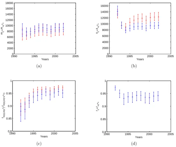
1990 1995 2000 2005 100 105 110 115 120 125 130 Years mk nn ,m <k nn> (a) 19900 1995 2000 2005 5 10 15 20 25 30 35 Years sk nn ,s<k nn > (b) 1990 1995 2000 2005 −1 −0.99 −0.98 −0.97 −0.96 −0.95 −0.94 −0.93 Years rk,k nn , rk,<k nn> (c) 1990 1995 2000 2005 0.93 0.94 0.95 0.96 0.97 0.98 0.99 1 Years rk nn,<k nn> (d)
Figure 4: Temporal evolution of the properties of the nearest neighbor degree k
inn
in the
1992-2002 snapshots of the real binary undirected ITN and of the corresponding maximum-entropy
ensembles with specified degrees. a) average of k
nniacross all vertices (red: real, blue: randomized).
b) standard deviation of k
inn
across all vertices (red: real, blue: randomized). c) correlation
coefficient between k
inn
and k
i(red: real, blue: randomized). d) correlation coefficient between k
innand < k
inn
>. The 95% confidence intervals of all quantities are represented as vertical bars.
2.2.2
Clustering
3
Commodity-specific binary undirected networks
5
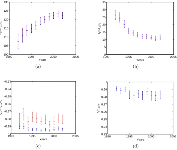
FIG. 2. Temporal evolution of the Average Nearest Neighbour Degree (knn
i ) from 1992 to 2002 and comparison with the
corresponding maximum-entropy ensembles with specified degrees and strengths (ECM). (a) average of knn
i across all vertices
(red: obs., blue: randomized); (b) standard deviation of kinnacross all vertices; (c) correlation coefficient between knni and ki;
(d) correlation coefficient between knni and hkinni. Red: observed values; blue: expected values. The 95% confidence intervals
of all quantities are represented as vertical bars.
linear correlation coefficient. Thus our choice of includ-ing the correlation coefficient (iii ) is mainly due to the need of comparing our results with previous studies, as we now discuss.
The analysis described above is shown in four figures (one for each structural property) of four panels each (one for each metric). Specifically, figs. 2, 3, 4 and 5 show the temporal evolution (time series) of the four metrics men-tioned above, for the Average Nearest Neighbour Degree, Binary Clustering Coefficient, Average Nearest Neigh-bour Strength and Weighted Clustering Coefficient re-spectively. For each property and each point in time, we also plot the associated 95% confidence intervals. Again, this kind of visualization coincides intentionally with that used in previous analyses of the same data, where the BCM [22] and WCM [33] were used. Our use of the same four metrics and the same four properties allows us to compare the performance of the ECM, i.e. of the com-bination of degrees and strengths, with that of the other
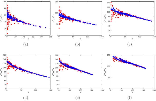
two null models where only one constraint is used. Figures 2 and 3 show that the time series of both aver-age value and standard deviation of the Averaver-age Nearest Neighbor Degree and Clustering Coefficient are all per-fectly replicated by the ECM predictions over time. The correlation coefficient (iii ) of both knn
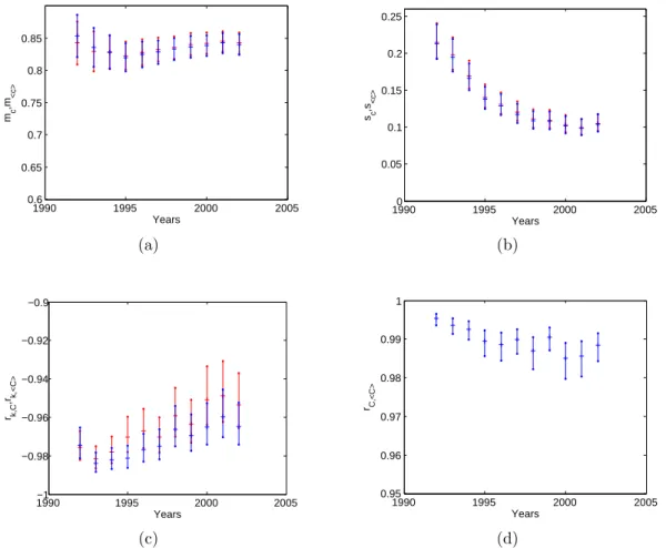
i and ci with ki is the only metric where there is some minor disagreement, however this cannot be interpreted as a statistically sig-nificant deviation, as we discussed. The tight agreement between observed and expected values over time is best confirmed by the correlation coefficient (iv ), which is al-ways very close to 1. All these results are perfectly in line with what is obtained using the BCM, i.e. when only the degree is enforced as a constraint, on the purely binary representation of the same data [22]. This means that, by simultaneously preserving degrees and strengths, the ECM does not diminish the ability of the BCM to predict the binary topology of the WTW (as we have seen in fig. 1, the ECM actually improves the already good fit of the
1990 1995 2000 2005 0.6 0.65 0.7 0.75 0.8 0.85 Years mc ,m <c> (a) 19900 1995 2000 2005 0.05 0.1 0.15 0.2 0.25 Years sc ,s<c> (b) 1990 1995 2000 2005 −1 −0.98 −0.96 −0.94 −0.92 −0.9 Years rk,C ,rk,<C> (c) 1990 1995 2000 2005 0.95 0.96 0.97 0.98 0.99 1 Years rC,<C> (d)
Figure 5: Temporal evolution of the properties of the clustering coefficient c
iin the 1992-2002
snapshots of the real binary undirected ITN and of the corresponding maximum-entropy
ensem-bles with specified degrees and strengths. a) average of c
iacross all vertices (red: real, blue:
randomized). b) standard deviation of c
iacross all vertices (red: real, blue: randomized). c)
correlation coefficient between c
iand k
i(red: real, blue: randomized). d) correlation coefficient
between c
iand < c
i>. The 95% confidence intervals of all quantities are represented as vertical
bars.
3.1
Average nearest neighbor degree
6
FIG. 3. Temporal evolution of the Binary Clustering Coefficient (ci) from 1992 to 2002, and comparison with the corresponding
maximum-entropy ensembles with specified degrees ans strengths (ECM). (a) average of ciacross all vertices (red: obs., blue:
randomized); (b) standard deviation of ci across all vertices; (c) correlation coefficient between ci and ki; (d) correlation
coefficient between ciand hcii. Red: observed values; blue: expected values. The 95% confidence intervals of all quantities are
represented as vertical bars.
BCM to the data).
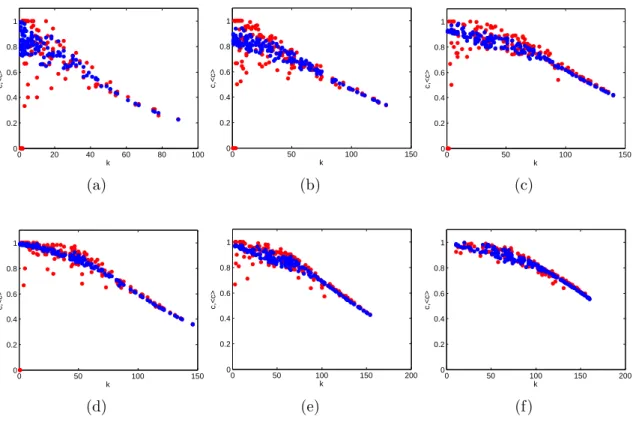
Figures 4 and 5 show that also for the weighted net-work properties there is an excellent agreement between the observed values and the corresponding expectations over the ECM, for the whole period. The ECM is able to accurately reproduce the temporal trends of the aver-age of both snn
i and cwi , as well as their standard devia-tion. The correlation (iii ) of these properties with node strength is also well replicated by the ECM in the whole period. Finally, the correlation coefficient (iv ) between observed and randomized properties is almost 1 all the time. These results are very different from what is ob-tained using the WCM on the same data [33]. Again, the WCM is completely unable to replicate the observed trends. The addition of purely binary information, em-bodied in the number of node partners, makes the ECM very powerful in predicting the higher-order properties of the WTW, throughout the temporal window considered.
C. Information-theoretic comparison
of the WCM and the ECM
Before proceeding to the analysis of individual layers of the trade multiplex, we perform an important check of the statistical appropriateness of the results obtained so far. This check is needed for the following reason. It is obvious that, by including more constraints, the ECM achieves a better fit than the WCM. However, in principle the gain in accuracy (better fit) might be smaller than the loss in parsimony (more parameters), i.e. the ECM might overfit the network. To rigorously make this assessment, we perform an information-theoretic comparison of the two models in terms of the achieved trade-off between accuracy and parsimony.
Information-theoretic criteria exist [60] to assess whether the increased accuracy of a model with more parameters comes at the price of an excessive loss of par-simony. The most popular choice is the Akaike’s Informa-tion Criterion (AIC), showing that the optimal trade-off between accuracy and parsimony is achieved by discount-ing the number of free parameters from the maximized
19905 1995 2000 2005 6 7 8 9 10 11x 10 6 Years ms nn ,m <s nn> (a) 19901 1995 2000 2005 2 3 4 5 6x 10 6 Years ss nn ,s<s nn> (b) 1990−1 1995 2000 2005 −0.8 −0.6 −0.4 −0.2 0 Years rs,s nn , rs,<s nn> (c) 1990 1995 2000 2005 0.95 0.96 0.97 0.98 0.99 1 Years rs nn,<s nn > (d)
Figure 9: Temporal evolution of the properties of the nearest neighbor strength s
inn
in the
1992-2002 snapshots of the real weighted undirected ITN and of the corresponding maximum-entropy
ensembles with specified strengths. a) average of s
inn
across all vertices (red: real, blue:
random-ized). b) standard deviation of s
inn
across all vertices (red: real, blue: randomized). c) correlation
coefficient between s
inn
and s
i(red: real, blue: randomized). d) correlation coefficient between s
innand < s
inn
>. The 95% confidence intervals of all quantities are represented as vertical bars.
3.4.2
Clustering
4
Commodity-specific weighted undirected networks
10
FIG. 4. Temporal evolution of the properties of the ANNS snn
i in the 1992-2002 snapshots of the observed undirected WTW
and of the corresponding maximum-entropy ensembles with specified degrees ans strengths: (a) average of snni across all vertices
(red: obs., blue: randomized); (b) standard deviation of snni across all vertices; (c) correlation coefficient between snni and si;
(d) correlation coefficient between snn
i and hsnni i. Red points stands for observed values, blue for the randomized ones; the
95% confidence intervals of all quantities are represented as vertical bars.
log-likelihood [60].
To compute AIC, we therefore first need to calculate the maximized log-likelihood of the two models. As we mentioned, the WCM can be obtained as a particular
case of the ECM by setting xi = 1 for all i, i.e. by
‘switching off’ the Lagrange parameters controlling for the degrees. The log-likelihood of the WCM is therefore the reduced function L(~1, ~y) of N variables, and is max-imized by a new vector ~y∗∗ 6= ~y∗, where (~x∗, ~y∗) stands for the solution of the ECM and (~1, ~y∗∗) for the solution of the WCM for the same observed network.
Given the maximized log-likelihood of our two compet-ing models, we calculate the size-corrected [60] version of AIC, denoted as AICc, as follows:
AICcECM ≡ −2L(~x∗, ~y∗) + 4N + 8N (2N + 1)
N2− 5N − 2 (27)
AICcW CM≡ −2L(~1, ~y∗∗) + 2N + 4N (N + 1)
N2− 3N − 2 (28)
The last term on the r.h.s. of both equations provides the
correction to AIC when the number of parameters is not negligible with respect to the sample cardinality (as a rule of thumb, when n/k < 40, n being the cardinality of the sample and k being the number of parameters [60]), thus further reducing the probability of overfitting. Notice
that, when n k2, the additional term converges to
0, recovering the standard form of AIC for the ECM
[41]. Precisely for this reason, AICc should be always
employed regardless of the value of n/k [60].
The model that achieves the best trade-off between ac-curacy and parsimony is the one with the smallest value of AICc. However, if the difference of the AICcvalues is small, the two models will still be comparable. A quan-titative criterion to statistically interpret the differences of AICc is given by the so-called Akaike Weights, which quantify the weight of evidence in favour of a model, i.e., the probability that the model is the best one among the
19900 1995 2000 2005 2000 4000 6000 8000 10000 12000 14000 16000 18000 Years mc w ,m <c w> (a) 19900 1995 2000 2005 2000 4000 6000 8000 10000 12000 14000 16000 Years sc w ,s<c w> (b) 1990 1995 2000 2005 0.8 0.85 0.9 0.95 1 Years rln(s),ln(c w) ,rln(s),ln(< c w>) (c) 1990 1995 2000 2005 0.8 0.85 0.9 0.95 1 Years rc w ,r< c w> (d)
Figure 10: Temporal evolution of the properties of the weighted clustering coefficient c
wi
in the
1992-2002 snapshots of the real weighted undirected ITN and of the corresponding
maximum-entropy ensembles with specified strengths. a) average of c
wi
across all vertices (red: real, blue:
randomized). b) standard deviation of c
wi
across all vertices (red: real, blue: randomized). c)
correlation coefficient between log(c
wi
) and log(s
i) (red: real, blue: randomized). d) correlation
coefficient between c
wi
and < c
wi>. The 95% confidence intervals of all quantities are represented
as vertical bars.
4.1
Average nearest neighbor strength
4.2
Weighted Clustering
5
Bosonic and Mixed case comparison
5.1
Average nearest neighbor degree
5.2
Clustering Coefficient
11
FIG. 5. Temporal evolution of the properties of the WCC cwi in the 1992-2002 snapshots of the observed undirected WTW and
of the corresponding maximum-entropy ensembles with specified degrees ans strengths: (a) average of cw
i across all vertices
(red: obs., blue: randomized); (b) standard deviation of cwi across all vertices; (c) correlation coefficient between c
w
i and si;
(d) correlation coefficient between cwi and hcwii. Red points stands for observed values, blue for the randomized ones; the 95%
confidence intervals of all quantities are represented as vertical bars.
(two) models considered. In our case, these weights read wECMAIC c ≡ e−AICECMc /2 e−AICECM c /2+ e−AICW CMc /2 (29) wAICW CMc ≡ 1 − wECM AICc. (30)
Given a real network, a low value of wECM
AICc will indicate that the addition of the degree sequence is redundant (the relevant local constraints effectively reduce to the strength sequence, so the standard WCM is preferable), while a high value of wECM
AICc will indicate that, in addition to the strength sequence, the degrees must be separately specified. We stress that the result of this procedure is not predictable a priori (it depends on the numerical values of {si} and {ki}) and can only be achieved after a comparison of the two model on the specific data at hand.
In Table II we show the results for the two competing models, for the particular year 2002. We also used the Bayesian Information Criterion (BIC), [60], which puts a higher penalty on the number of parameters. Both
criteria yield (up to machine precision) a unit probability that the ECM is the best model. This confirms that the addition of the degree sequence as a constraint is non-redundant and extremely informative for the prediction of the WTW properties. We systematically found the same result for all temporal snapshots considered in sec. III B and all commodity classes that will be illustrated in sec. III D (values not shown for brevity).
The above finding implies that the world trade mul-tiplex is yet another system consistent with the ‘irre-ducibility conjecture’ we proposed in ref. [41]. This con-jecture states that, in real-world weighted networks, the strengths are not necessarily more informative than the degrees; rather, they are a complementary piece of infor-mation. Strengths and degrees are therefore ‘irreducible’ to each other, because they constrain the network in fun-damentally different ways.
An important macroeconomic implication is that any model aimed at reproducing the WTW (either statically, over time, and/or across its layers) should not discard any of the two quantities. This conclusion sets an
im-portant challenge for future models of trade, given that most models in the literature, and most notably Grav-ity Models [39, 40], mainly focus on weighted properties (trade volumes) and largely discard purely topological information.
D. Multiplex analysis:
commodity-specific trade networks
We conclude our empirical analysis by studying the individual networks formed by imports and exports of single (classes of) commodities.
As we described in sec. II A, our data set resolves the trade multiplex into C = 97 layers. While it is unfeasible to replicate the analysis described so far on each of the
C × T = 97 × 11 = 1067 networks resulting from the
evolution of the C layers over T years, we selected the same subset of layers as in refs. [22, 33]. This choice allows us to gain information about the performance of the ECM on layers with a broad range of sparseness and edge weight: while the aggregate WTW considered above is a highly dense network (with density around 0.5) with large total weight, the commodities we selected vary con-siderably in their intensity and level of connectivity. The selection includes the two least traded commodities (in terms of total trade value, i.e. total edge weight) in the entire data set (‘Arms and ammunition’, c = 93, and ‘Coffee, tea, mate & spices’, c = 9), two intermediate ones (‘Plastics’, c = 39, and ‘Optical, photographic, cin-ematographic, measuring, checking, precision, medical or surgical instruments’, c = 90), the most traded one (‘Nu-clear reactors, boilers, machinery and mechanical appli-ances’, c = 84), plus the network formed by combining all the top 14 commodities described in sec.II A together (see Table I for details). The last sub-network represents an intermediate level of aggregation between single com-modities and the completely aggregated data analysed in sec. III A. The six (classes of) commodities described above, plus the fully aggregated network itself, form a set of seven (combinations of) layers in increasing order of trade intensity, link density, and aggregation.
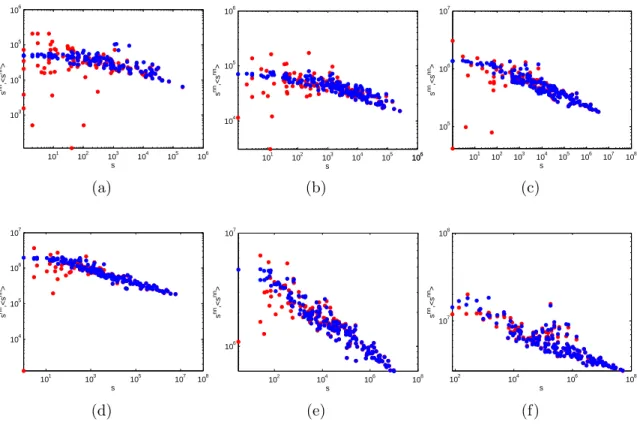
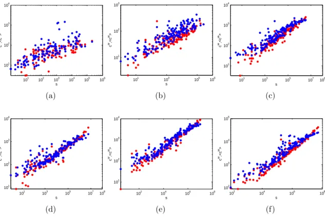
We consider the scatter plots of both binary and weighted higher-order properties for the 2002 snapshot of the above layers, as we did in ref.III A for the aggre-gate network. This is shown in figs. 6, 7, 8 and 9 for the Average Nearest Neighbour Degree, Binary Cluster-ing Coefficient, Average Nearest Neighbour Strength and Weighted Clustering Coefficient respectively.
Remark-AICc BIC wAICc wBIC
WCM 209, 972 211, 179 0 0
ECM 165, 731 168, 137 1 1
TABLE II. AICcand BIC values, along with the associated
AICc and BIC weights, for the two null models (WCM and
ECM) applied to the WTW in 2002.
ably, we find that the results obtained in our aggregated analysis also hold for individual commodities, indepen-dently of the level of aggregation. Also for the temporal evolution and information-theoretic analysis of the sys-tem, our results are very similar to those found for the aggregate network in secs. III B and III C respectively, but are not shown here for the sake of brevity.
The binary results confirm, and slightly improve, the performance of the BCM on the same data [22]. However, the excellent agreement between observed and random-ized weighted properties in the commodity-specific case is more surprising and represents a marked improvement with respect to the predictions of the WCM for the same system [33]. The case of the weighted clustering coef-ficient is particularly interesting in this sense. Indeed, while for the aggregate network the WCM gives a reason-able prediction of (only) this quantity (see fig. 1), this outcome is not robust to disaggregation: individual lay-ers of the empirical multiplex show a deviation from the WCM, which incresases with the sparseness of the layer [33]. On the contrary, fig. 9 shows that the ECM ac-curately replicates the observed clustering, as well as all the other properties under investigation, for every level of disaggregation.
In general, we observe a slightly worse agreement in layers with smaller density/volume (this is especially true for the weighted properties). However, this appears to be mainly due to the fact that the empirical scatter plots associated with less traded goods are more dispersed (due to less statistics). As expected, this effect is even more pronounced for the weighted quantities, because the range of allowed values for the strength is wider than that for the degree.
IV. DISCUSSION
We now discuss our result in the light of various lines of research in economics. In particular, we focus on the role of local properties in economic networks and on the rela-tion between our results and the established knowledged about intensive and extensive margins of trade.
A. The role of local properties in economic
networks
In economic and financial networks, the total strength of the connections reaching a node has generally an im-portant meaning, such as the size of supply and demand, import and export, or financial exposure. Hence, gen-erating random ensembles of networks matching the ob-served strengths of all nodes is crucial in order to detect interesting deviations of a known empirical network from economically meaningful benchmarks, to reconstruct the most likely structure of an unknown network from purely local information, or finally to define a model of economic networks specified by node-specific properties.
0 20 40 60 80 100 0 20 40 60 80 100 k k nn,<k nn > (a) 0 50 100 150 0 50 100 150 k k nn ,<k nn > (b) 0 50 100 150 0 20 40 60 80 100 120 140 k k nn ,<k nn> (c) 0 50 100 150 0 20 40 60 80 100 120 140 160 k k nn ,<k nn > (d) 0 50 100 150 200 0 20 40 60 80 100 120 140 160 k k nn ,<k nn > (e) 0 50 100 150 200 0 50 100 150 k k nn ,<k nn > (f)
Figure 1
FIG. 6. Average Nearest Neighbour Degree (knni ) versus node degree (ki) in the 2002 snapshots of the commodity-specific
(disaggregated) versions of the observed binary undirected WTW (red points), and corresponding average over the maximum entropy ensemble with specified degrees and strengths (blue points): a) commodity 93; b) commodity 09; c) commodity 39; d) commodity 90; e) commodity 84; f) aggregation of the top 14 commodities (see table I for details). From a) to f), the intensity of trade and level of aggregation increases.
Our results show that, in order to correctly reproduce the whole structure of the WTW as a weighted network, the degree sequence must be constrained in addition to the strength sequence. From the general point of view of network reconstruction, these findings consolidate and widely extend the results in [41]. We confirmed the ef-fectiveness of the ECM in reproducing the higher-order properties of the WTW starting from local constraints, and succesfully tested the robustness of the model with respect to several temporal snapshots and levels of ag-gregation. So, while the strength sequence (a weighted constraint) turns out to be uninformative about the nary topology of the WTW, the degree sequence (a bi-nary constraint) plays a fundamental role in reproducing its weighted structure. This highly asymmetric role of binary and weighted constraints is a non-trivial result.
From an economic perspective, the fact that purely local information is enough in order to reproduce the large-scale structure of the WTW implies that parsimo-nious models of international trade can largely discard additional mechanisms besides those accounting for the number of partners and total trade of world countries. The importance of reproducing and/or explaining the de-grees of all world countries, first pointed out in [22], is confirmed by our study, and shown to hold even when
one considers the weighted representation of the WTW. This strengthens the view that theories and models of trade, when aiming at explaining the international net-work structure, should seriously focus on the number of trade partners of countries as an important target quan-tity to replicate.
Of course, the above considerations leave an important point open, namely the role played by other properties of (expected) economic relevance in shaping the struc-ture of the international trade network. For instance, Gravity Models [37–40] predict that both country-specific (mainly the GDP) and dyadic quantities, such as geo-graphic distance (which is a proxy of trade resistance) and other extra factors (such as common currency, com-mon language, borderding conditions, etc.), do play an important role. The GDP is directly related (and roughly proportional) to the total trade of a country, i.e. its strength [29, 61]. It is also related to the number of trade partners, i.e. the degree, in a highly non-linear way [17]. So, by controlling for both strengths and degrees, our ap-proach is indirectly controlling for the GDP of countries as well. The surprising agreement between our model and the data does not however imply that the other aforemen-tioned dyadic factors (involving pairs of countries) are unimportant. Rather, our analysis shows that, among
0 20 40 60 80 100 0 0.2 0.4 0.6 0.8 1 k c,<c> (a) 0 50 100 150 0 0.2 0.4 0.6 0.8 1 k c,<c> (b) 0 50 100 150 0 0.2 0.4 0.6 0.8 1 k c,<c> (c) 0 50 100 150 0 0.2 0.4 0.6 0.8 1 k c,<c> (d) 0 50 100 150 200 0 0.2 0.4 0.6 0.8 1 k c,<c> (e) 0 50 100 150 200 0 0.2 0.4 0.6 0.8 1 k c,<c> (f)
Figure 1
FIG. 7. Binary Clustering Coefficient (ci) versus node degree (ki) in the 2002 snapshots of the commodity-specific
(disaggre-gated) versions of the observed binary undirected WTW (red points), and corresponding average over the maximum entropy ensemble with specified degrees and strengths (blue points): a) commodity 93; b) commodity 09; c) commodity 39; d) com-modity 90; e) comcom-modity 84; f) aggregation of the top 14 commodities (see table I for details). From a) to f), the intensity of trade and level of aggregation increases.
the country-specific factors, the ones that only affect the strengths are definitely less informative than those that impact both strengths and degrees. Adding the dis-tances, or other dyadic factors, can in principle lead to an even better agreement between model and data. On the other hand, it is interesting to notice that geographic dis-tances are sometimes outperformed by purely topological properties (such as the reciprocity [58]) in explaining the structure of the WTW, and in general Gravity Models are much less effective than maximum-entropy ensembles in reproducing the binary structure of the WTW [39, 40]. The main reason for this ineffectiveness is that, depend-ing on their specification, Gravity Models tend to predict a network that is either too dense (in the simplest setting, even fully connected [40]) or too topologically different from the observed WTW [39].
B. Intensive and extensive margins
Another series of important economic considerations concerns the relationship between our findings and the so-called extensive and intensive margins of trade. These two concepts, first introduced by Ricardo [47], are widely used in economics, and should not be confused with the
notion of intensive and extensive variables in statistical physics and thermodynamics. In the context of inter-national trade, extensive and intensive margins refer to tendency of the network to evolve through the creation of new trade connections or through the reinforcement of existing ones respectively [48, 49].
Even if both margins are known to be relevant, nei-ther a systematic treatment of their role in the predic-tion of internapredic-tional trade relapredic-tionships, nor an agree-ment on their relative importance can be found in the economic literature. Some works agree on the relevance of extensive margins. For instance, a cross-country anal-ysis reveals that extensive margins account for the 60% of exports of the larger economies [62], and another study shows that increasing extensive margins means augment-ing exports of developaugment-ing countries [63].
At the same time, a large body of work stresses the relevance of intensive margins. For instance, intensive margins represented a fundamental factor in the period 1970-1990 [48, 64] and have been particularly relevant for China’s exports growth in the period 1992-2005 [65] and for Colombian countries’ exports [66]. It has also been claimed [67] that the majority of trade growth is due to the intensive margin, rather than the extensive one. This view stresses the importance to focus on a
101 102 103 104 105 106 103 104 105 106 s s nn ,<s nn > (a) 101 102 103 104 105 101066 104 105 106 s s nn ,<s nn > (b) 101 102 103 104 105 106 107 108 105 106 107 s s nn ,<s nn > (c) 101 103 105 107 108 104 105 106 107 s s nn,<s nn> (d) 102 104 106 108 106 107 s s nn ,<s nn > (e) 102 104 106 108 107 108 s s nn ,<s nn > (f)
Figure 1
FIG. 8. Average Nearest Neighbour Strength (snni ) versus node strength (si) in the 2002 snapshots of the commodity-specific
(disaggregated) versions of the observed binary undirected WTW (red points), and corresponding average over the maximum entropy ensemble with specified degrees and strengths (blue points): a) commodity 93; b) commodity 09; c) commodity 39; d) commodity 90; e) commodity 84; f) aggregation of the top 14 commodities (see table I for details). From a) to f), the intensity of trade and level of aggregation increases.
dynamical comparison (e.g. introducing the concepts of ‘survival’ and ‘deepening’ to characterize export relation-ships) rather than on a standard static approach.
The controversial results existing in the literature ap-pear to be mainly due to the different levels at which the two margins are examined [67]: some works define extensive margins at the country-product level, others at the product level, others at the country level. This problem, together with the composite effect of interna-tional changes on trade, can determine mixed and contra-dictory results. For example, trade liberalization affects trade flows in two ways. On the one hand, since trade becomes less costly, the trade volumes increase (intensive margin at product level). On the other hand, more firms trade and more goods are traded (extensive margin both at product and country-product level). It has been ob-served [38] that the elasticity of substitution should also be taken into account, because it has opposite effects on the two margins: high elasticity makes the intensive margin more sensitive to changes in trade barriers (trade costs), whereas the extensive margin is less sensitive to this effect.
To the best of our knowledge, in the economic liter-ature there has been no systematic analysis of the pre-dictive power of extensive and intensive trade margins
so far. Starting from one snapshot of the international trade network, is the knowledge of the growth of trade along the intensive and/or extensive margin enough to predict the structure of the network at a later time?
Even if our results cannot fully answer such question, they suggest a plausible scenario. We first note that a change in the degree (number of partners) of a country implies that the network is evolving along the extensive margin of trade. On the other hand, a change in the strength (total volume) can be either be due to changes in the number of partners or to changes of the amount of trade for existing links. This means that, while changes in the degree only reflect the extensive margin, changes in the strength reflect both the extensive and intensive mar-gins: this is a second asymmetry between the different pieces of information encoded into the degrees and the strengths. It is also another indication that the WCM, by enforcing the strengths alone, cannot distinguish be-tween the two margins, while the ECM can isolate the extensive information (degrees) from the combined one (strengths).
Our findings imply that, if the structure of the interna-tional trade network is known at time t, and if the growth (or decrease) of both strengths and degrees from time t to time t + ∆t is also known, then it is possible to predict