Robust optimization in multi-operators microwave backhaul networks

(1)

HAL Id: hal-00870931

https://hal.inria.fr/hal-00870931

Submitted on 8 Oct 2013

HAL is a multi-disciplinary open access

archive for the deposit and dissemination of

sci-entific research documents, whether they are

pub-lished or not. The documents may come from

teaching and research institutions in France or

abroad, or from public or private research centers.

L’archive ouverte pluridisciplinaire HAL, est

destinée au dépôt et à la diffusion de documents

scientifiques de niveau recherche, publiés ou non,

émanant des établissements d’enseignement et de

recherche français ou étrangers, des laboratoires

publics ou privés.

Robust optimization in multi-operators microwave

backhaul networks

Christelle Caillouet, David Coudert, Alvinice Kodjo

To cite this version:

Christelle Caillouet, David Coudert, Alvinice Kodjo. Robust optimization in multi-operators

mi-crowave backhaul networks. 4th Global Information Infrastructure and Networking Symposium, Oct

2013, Trento, Italy. pp.1-6. �hal-00870931�

(2)

Robust optimization in multi-operators microwave

backhaul networks

Christelle Caillouet, David Coudert and Alvinice Kodjo

Univ. Nice Sophia Antipolis, CNRS, I3S, UMR 7271, 06900 Sophia Antipolis, France Inria, Sophia Antipolis, France

Abstract—In this paper, we consider the problem of sharing the infrastructure of a backhaul network, called fixed broadband wireless network using microwave links, for routing. We inves-tigate in particular on the revenue maximization problem for the physical network operator (PNO) when subject to stochastic traffic requirements of multiple virtual network operators (VNO) and prescribed service level agreements (SLA). We use robust optimization to study the tradeoff between revenue maximization and the allowed level of uncertainty in the traffic demands. We propose a mathematical programming formulation of our robust optimization problem using mixed integer linear programming. This model takes into account end-to-end traffic delays as example of quality-of-service requirement in a SLA. To show the effectiveness of our model, we present a study on the price of robustness, i.e. the additional price to pay in order to obtain a feasible solution for the robust scheme, on realistic scenarios.

Keywords-Wireless backhaul networks, Γ-robust network op-timization, infrastructure sharing, MILP.

I. INTRODUCTION

Fixed broadband wireless (FBW) communications is a promising technology for implementing wireless backhaul net-works, the portion of the network infrastructure that provides interconnection between access and core networks [1]. It uses microwave radio transmission [2] for establishing high-speed point-to-point connections, usually employing highly direc-tional antennas in clear line-of-sight and operating in licensed frequency bands [3], [4], [5]. The microwave technology has the advantage to be rapidly and cost-effectively deployed compared to optical fibers and is especially interesting for reaching remote locations or deploying private and isolated networks in urban area where the cost of other solutions might be prohibitive. It also offers very good capacity (up to 1 Gbits/sec. on each link) and delays characteristics compared to all others technologies possible on this part of network.

FBW networks have received little attention from the sci-entific community while having a huge interest from network operators. For instance, with the advent of the 4thGeneration (4G) of mobile networks, mobile operators have to make huge investment to upgrade their physical networks. But, with the traffic demand increase triggered by the new services offered on 4G networks, the capacity bottleneck has moved from the radio interface towards the backhaul network [6], [4]. Therefore, the need for optimizing FBW networks is twofold. On the one hand, wireless telecommunication operators have to offer maximum territory coverage with high quality of service and at low cost to attract clients and so make profits.

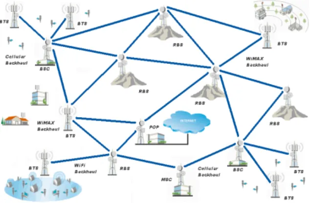
Fig. 1. Example of Wireless backhaul network

On the other hand, revenue maximization is strongly impacted by the deployment and operation costs of both the wireless base stations and the backhaul networks.

To increase profits in FBW networks, recent studies have considered the reduction of both the capital and operational costs. For instance, [7], [3] address the capacity planning problem in FBW networks using microwave links which are prone to external factors (e.g., weather conditions). Through a joint optimization of data routing and bandwidth assignment to links, they were able to reduce both the cost of antennas and the total renewal fees of licenses. Moreover, the problem of reducing the overall power consumption of the FBW network, which is part of the expenses, has been considered in [8].

In this work, and following the actual separation between infrastructure and services, we distinguish between two kinds of operators: the Physical Network Operator (PNO) that owns and operates the FBW network (antennas, radio links, etc.) and the Virtual Network Operator (VNO) that rents capacity from the PNO to deliver services to its clients. In fact, many network operators are of both kinds since it is hardly cost effective to fully deploy its own infrastructure for achieving full coverage of a country. Typically, remote areas have longer return of investments than dense cities. This in addition with local and national regulation of wireless transmissions aiming at reducing the radio smog are strong incentives for sharing infrastructure and so optimizing investments and revenues [9]. For instance, wireless base stations in remote areas with low traffic are often shared between operators to reduce investment, and most of the high points where to install antennas are rented to dedicated companies.

(3)

We consider that the service level agreement (SLA) signed between the PNO and a VNO includes not only quality-of-service (QoS) requirements such as delays and satisfiability among concurrent flows, but also the capacity requirements over time. Motivated by an efficient computation of the optimal solution of our problem, we derive a mathematical formulation of the infrastructure sharing with SLA problem with the objective of maximizing the PNO revenue. We then extend the formulation considering uncertain traffic demands of the VNOs. To do that, we use robust optimization that is a new approach in mathematical optimization to deal with uncertainty [10]. It is related with stochastic programming, in that some of the parameters are random variables, except that feasibility for all possible realizations (called scenarios) is replaced by a penalty function in the program. In other words, the goal of robust optimization is to optimize against the worst instances that might arise. We consider a parameter Γ, introduced by Bertsimas and Sim [11], that corresponds to the degree of robustness, i.e. the level of conservatism of the robust solution. This allows a better flexibility than traditional too conservative robust models like the hose model [12]. From a practical point of view, it is unlikely that all the VNO traffic requirements reach their peak value at the same time. Therefore we consider the case where the number of demands deviating from their mean value is bounded by Γ. Making Γ vary from 0 to the total number of demands allows us to study the so-called price of robustness, i.e. the additional price to pay in order to obtain a feasible solution for the robust scheme.

We carefully define the problem and formulate it when demands are considered static in Section II, while in Sec-tion III we present its robust formulaSec-tion using integer linear programming, in which demand requirements are modeled as random variables. We report on computational results in Section IV and conclude with a perspective problem.

II. PROBLEM DEFINITION AND STATIC FORMULATION

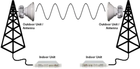
We consider a fixed broadband wireless network where each node represents a tower on which one or many Base Transciever Stations (BTS) are installed. Each BTS consists of three basic components: an indoor unit which performs all digital processing operations and provides advanced network-ing capabilities such as routnetwork-ing and load balancnetwork-ing; an outdoor unit which houses all the radio frequency (RF) modules for converting a carrier signal to a microwave signal; and the antenna used to transmit and receive the signal into/from free space as shown in Fig. 2 . Two BTS located on different towers can be connected to each other with point-to-point wireless links, and two different BTS located on the same tower are connected through a switch link connecting their indoor units. We define our problem on a digraph G = (V, E) where V represents a set of towers and each link (u, v) ∈ E represents a fixed radio directed link between an antenna of a BTS located on node u to an antenna of a BTS located on node v. To each link (u, v) is associated a defined capacity value Cuv. We are

also given a set of n different VNOs and the traffic demand for a VNO q is represented by a set Dq = {(skq, tkq, dkq), k =

!

Fig. 2. Example of Wireless point-to-point link

1, . . . , |Dq|, q = 1, . . . , n} with skq, tkq and dkq respectively the

source, the destination and the volume of the kth_{demand of}

the qth_VNO.

The infrastructure sharing problem includes a SLA (Service Level Agreement) option including conditions on the end-to-end transmission delay for each traffic demand of each VNO. In order to efficiently compute the delay in the backhaul network, we made the following two assumptions. Firstly, the propagation delay on a link (delay needed for a symbol to reach the reception antenna from the emission one) is considered to be negligible regarding to its transmission delay in a router (delay needed to decode it, to send it from the antenna to the indoor unit, to treat it in the router, to send it to another indoor unit, to re-code it and to send it to the antenna for emission). This hypothesis is based on the fact that in microwave networks, propagation delays are in order of tens of microseconds (µs) while transmission delays are in order of milliseconds (ms) [5]. Secondly, the transmission delay of a unit of traffic demand in a router of the infrastructure is known by advance and denoted by τ . It corresponds to a maximum value corresponding to the worst case where there is congestion in the router. We then assume that each VNO has its own QoS policy based on a maximum end-to-end transmission delay of value Tq, q = 1..n. So we consider that

a demand (sk

q, tkq, dkq) of a VNO q is satisfied through our

backhaul network if and only if the volume of traffic demand dk

q can be totally routed in the network from the source node

sk

q to the destination node dkq, respecting the capacity available

on each link of the routing path, and with a total transmission delay less or equal to Tq. In turn, we consider that a VNO

satisfaction is met (or that a VNO can be served) if and only if at least a percentage β of its total number of demands are satisfied (remaining demands are served in best effort mode). Considering that a PNO increases its revenue every time it satisfies a VNO, the main purpose of our problem is to maximize the total revenue on this network, with respect to the delay and satisfiability constraints for each VNO.

Let Xk

q,uv, ∀{u, v} ∈ E, k = 1, · · · |Dq|, q = 1, · · · , n be a

binary variable representing whether or not the kth demand of the qth VNO is routed through the link (u, v). The binary variables gkq and aq denote respectively the satisfaction of the

kth _{demand of the q}th _{VNO, and the overall satisfaction of}

(4)

From all considerations above, we formulate the problem with the following integer linear model:

max n X q=1 Rqaq (1) s.t. X v/(u,v)∈E X_q,uvk − X v/(v,u)∈E X_q,vuk =      gk q if u = skq, −gk q if u = tkq, 0 otherwise ∀u ∈ V, k = 1 . . . |Dq|, q = 1 . . . n (2) n X q=1 |Dq| X k=1 dk_q X_q,uvk ≤ Cuv ∀ (u, v) ∈ E (3) τ · X (u,v)∈E X_q,uvk ≤ Tq.gqk ∀k = 1...|Dq|, q = 1...n (4) |Dq| X k=1 g_qk≥ β|Dq|aq ∀ q = 1 . . . n (5) aq, Xq,uvk , g k q ∈ {0, 1} (6)

The problem aims to maximize the total revenue of the network where Rqrepresents the revenue associated to VNO q.

Constraints (3) corresponds to the link capacity constraints limiting the total amount of flow routed on a link, while (2) ensures that the demand is routed on at most one path when the demand can be satisfied. Constraints (4) are used to determine if a demand k is satisfied or not regarding to the delay recommendation of the qth_{VNO. The transmission delay of a}

demand is calculated as the product of the maximum delay at a node τ by the number of traffic nodes in which this demand is routed from the source to the destination. The binary variable gk_q is set to 0 if the transmission delay of a demand is greater than the one allowed by the VNO, and consequently forces the associate flow variables to 0. Finally, Constraints (5) decide if a VNO can be satisfied or not depending on the percentage β. One can add to this model Constraint (7) that forces all demand satisfaction variables for a VNO to 0 if this VNO can not be satisfied. But we decide here not to put it in our model in order to evaluate the percentage of demands that can be satisfied for a VNO even if all its requirements are not met.

g_qk≤ aq ∀ k = 1...|Dq|, q = 1...n (7)

In the next section, we extend our model by taking into account the variations of traffic load happening in telecommu-nications networks. The new model will be robust against these variations and will help to cost-effectively serve the VNOs.

III. ROBUST MODEL

In the model described in the previous section, we consider that all traffic demands are static. However in telecommu-nication networks, traffic fluctuates among time. In order to take these variations into account in our optimization model, we define a new approach based on robust optimization with uncertainty parameter. More precisely in our approach, we consider the influence of demand uncertainty on the quality and the feasibility of the model for infrastructure sharing

with SLA. So, we now model the traffic demand dkq as

random variables taking their values in a symmetric interval h ¯_dk

q− ˆdkq, ¯dkq + ˆdkq

i

, where ¯dk

q is called the nominal value and

ˆ dk

q the maximum deviation value.

We assume that at most a few number of demands fluctuate at the same time. Indeed, it is unlikely to have all the traffic demands of all the VNOs reaching their peak value simultaneously. This encourage to use the method of Bertsimas and Sim [11] that is less conservative than other robust models. We thus denote by Γ, called the robustness parameter, the maximum number of demands that can deviate simultaneously in the network and reach their peak value ¯dk

q + ˆdkq. Let

0 ≤ Γ ≤Pn

q=1|Dq| be the possible values of Γ.

Integrating the robust optimization approach into the linear programming model (1)-(6), only Constraints (3) has to be modified. Indeed, because of the demand uncertainties, (3) will now be transformed into Constraints (8) where D = ∪k=1...|Dq|

q=1...n

{(sk

q, tkq, dkq)} is the union set of all traffic demands. n X q=1 |Dq| X k=1 ¯ dk q X k q,uv+ max {S/S⊆D,|S|=Γ} X (sk q,tkq,dkq)∈S ˆ dk qX k q,uv≤ Cuv ∀ (u, v) ∈ E (8) Based on the new robust approach developed in [11] and given X_q,uvk for (u, v) ∈ E and Γ, the maximum part of the Constraints (8) can be re-written in a compact formulation as follows: δ(X, Γ) = max {S/S⊆D,|S|=Γ} X (sk q,tkq,dkq)∈S ˆ dk q X k q,uv = max n X q=1 |Dq| X k=1 ˆ dk q X k q,uvZ k q,uv (9a) s.t. n X q=1 |Dq| X k=1 Z_q,uvk ≤ Γ [σuv] (9b) 0 ≤ Z_q,uvk ≤ 1 ∀ q = 1 . . . n, k = 1 . . . |Dq| [ρkq,uv] (9c) where variable Zk

q,uv indicates which percentage of deviation

occurs for demand dkq while (9b) is used to limit the size of

the set S. By using the strong duality theorem [13] and the dual variables σuv, ρkq,uv of the precedent model, we get :

δ(X, Γ) = min n X q=1 |Dq| X k=1 ρkq,uv+ Γσuv (10a) s.t. σuv+ ρkq,uv ≥ ˆdkq X k q,uv ∀q = 1 . . . n, k = 1 . . . |Dq| (10b) σuv, ρkq,uv ≥ 0 ∀q = 1 . . . n, k = 1 . . . |Dq| (10c)

From this, we can write the Robust model of our original problem as follows: max n X q=1 Rqaq

(5)

Subject to Equations (2), (4), (5), (6), and n X q=1 |Dq| X k=1 dk_q X_uv,qk + n X q=1 |Dq| X k=1 ρk_q,uv+ Γσuv≤ Cuv ∀ (u, v) ∈ E (11a) σuv+ ρkq,uv ≥ ˆdkq X k q,uv ∀q = 1 . . . n, k = 1 . . . |Dq| (u, v) ∈ E (11b) σuv, ρkq,uv ≥ 0 ∀q = 1 . . . n, k = 1 . . . |Dq| (u, v) ∈ E (11c) IV. COMPUTATIONAL RESULTS

A. Computation settings and test instances

Given the absence of topology instances for microwave backhaul networks available in the literature, we constructed instances for our problem using networks topologies taken from the SNDlib library [14]. We used the network topology and the traffic matrix of four instances from that library, namely Abilene, Atlanta, Dfn, and Polska, on which we applied a scaling factor on the nominal traffic volumes to cope with links capacities of 1 Gbits/sec. (best possible link capacity using nowadays microwave technology). We have then randomly defined the number of traffic demands Dq

for VNO q, the revenue Rq for a satisfied VNO q (relative

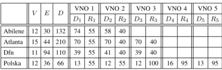
numbers to be multiplied for instance by 1000$ per year), and split the traffic demands arbitrarily into several groups, each associated to a VNO. All settings have been reported in Table I. For each instance, we set the possible deviation to 60%, 50%, 50% and 40% of the nominal traffic demands respectively for Abilene, Atlanta, Dfn and Polska. Finally, we set τ = 1 and β = 90% such that a VNO is satisfied only if few of its demands can not be correctly routed.

B. Results and discussion

We solved the constructed instances for all possible values of Γ using the Cplex solver [15] on a computer equiped with a 2.9 Ghz Intel Core i7 CPU and 8 GB of RAM. We have set a time limit of 2 hours for solving an instance. We get optimal solutions for almost all instances and a small optimality gap for few of them. We analyse our results in the next subsections, starting with the price of robustness.

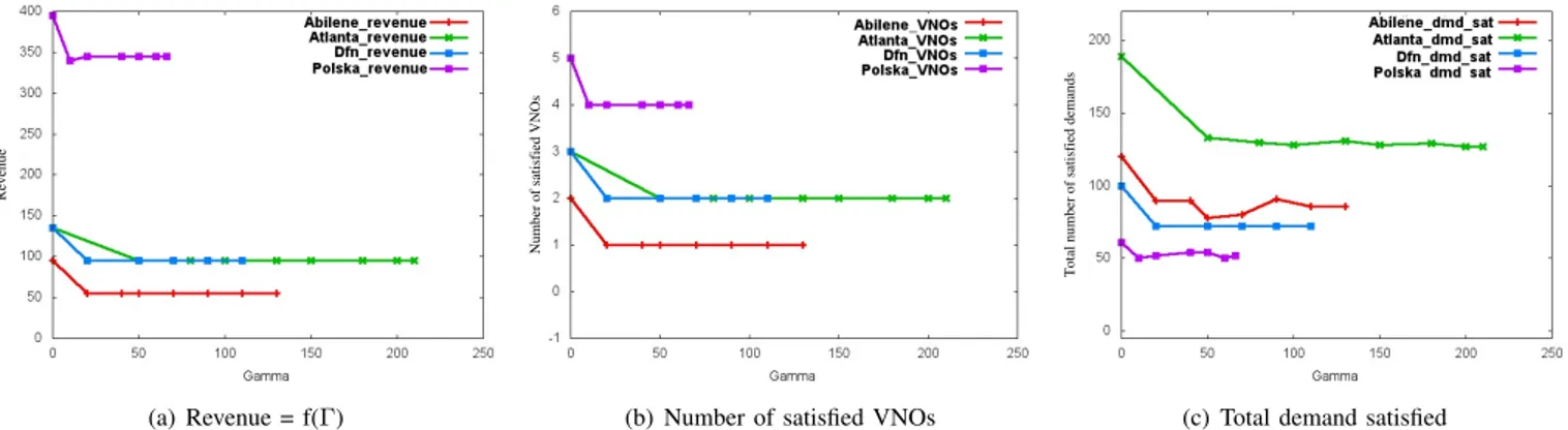
1) Price of robustness: We have reported in Fig. 3 for each instances the evolution of the revenue, the number of satisfied VNOs, and the total number of satisfied demands when Γ increases. The general shape of the plots is similar for all instances. When Γ = 0, no traffic deviation is allowed, and so the reported results are for the nominal traffic demands, and when Γ = |D|, all traffic demands are at their peak.

In Fig. 3(a) we observe that the revenue decreases as soon as some traffic variations are allowed, and that it quickly reaches a plateau which shows us that above a certain value, the number Γ of uncertain demands does not have any impact on the VNO satisfaction. This is an important indication for the PNO in the tradeoff between investment for increasing the capacity of the network and potential revenue increase

TABLE I TEST INSTANCES SETTINGS

V E D VNO 1 VNO 2 VNO 3 VNO 4 VNO 5 D1 R1 D2 R2 D3 R3 D4 R4 D5 R5

Abilene 12 30 132 74 55 58 40

Atlanta 15 44 210 70 55 70 40 70 40 Dfn 11 94 110 39 55 41 40 39 40

Polska 12 36 66 13 55 12 55 12 100 16 95 13 95

(difference between the revenue for Γ = 0 and the plateau). In fact, in the robust model, the sum of the peak traffic requirements increases with Γ. Since the link capacities are fixed, it is no longer possible to accept all the traffic demands (as shown in Fig. 3(c)) and so only a subset of the VNOs can be satisfied as shown with Fig. 3(b).

Recall that our model tries to maximize the total number of satisfied demands in the network, even if at the end, the VNO itself cannot be satisfied due to the percentage β defined in the SLA. This can be observed in Fig. 3(c). The number of satisfied demands of an unsatisfied VNO depends mainly on the residual capacity in the network when demands of the satisfied VNO are well routed, which in turn depends on the volume of these last demands. Figs. 4(a), 4(b), 4(c) and 5 present the repartition of the satisfied demands per VNO respectively in Abilene, Atlanta, Polska, and Dfn networks when the robustness parameter Γ increases. For instance, the changes in the subset of satisfied VNOs when Γ increases can be observed in Fig. 4(b). When Γ ≥ 50, only two VNOs can be satisfied, either VNO1 and VNO2, or VNO1 and VNO3, and the variations are explained by the evolution of the total number of satisfied demands, which also depends on the volume of these demands. The plateau on the revenue observed in Fig. 3(a) is explained by that fact that VNO2 and VNO3 provide the same revenue for the PNO. Clearly, if the revenue for VNO3 was higher than the revenue for VNO2, the model would always choose the subset with VNO1 and VNO3 since it can be satisfied for all values of Γ.

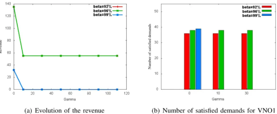
2) Impact of the parameter β: We now investigate on the impact of the parameter β on the satisfaction of VNOs when using the worst case of the QoS policy. Recall that this parameter expresses the percentage of traffic demands to satisfy in order to accept the VNO. Other traffic demands can be served on a best effort basis.

We have solved the Dfn instance with different values of β: 92%, 96%, and 99%. The results are reported in Figs. 6(a) and 6(b). We observe in Fig. 6(a) a drastic drop down of the revenue when β increases. Recall that the revenue for β = 90% reported in Fig. 3(a) was even higher. This indicates that this stronger satisfaction requirement of the VNOs forces the PNO to accept less VNOs. For instance, when β = 99% and for values of Γ ≥ 10, none of the VNO can be satisfied.

In Fig. 6(b), we observe that the percentage of satisfied traffic demands for VNO1 is larger when β = 96% than when β = 92%. Indeed, the first objective of our model is to maximize the revenue and so to choose the right number of

(6)

Revenue

(a) Revenue = f(Γ)

Number of satisfied VNOs

(b) Number of satisfied VNOs

Total number of satisfied demands

(c) Total demand satisfied Fig. 3. Evolution of the revenues (3(a)), number of satisfied VNOs (3(b)), and total number of satisfied demands (3(c)) as a function of Γ.

Number of satisfied demands per VNO

(a) Abilene

(b) Atlanta

(c) Polska Fig. 4. Repartition of satisfied demands per VNO when Γ increases for Abilene, Atlanta, and Polska.

satisfied VNO. Then, since we never force variables gkq to zero

if VNO q is not satisfied, the model will route many traffic demands independently of the satisfaction of the VNOs. This can also be observed in Fig. 4(a) where although VNO1 is the only satisfied VNO as soon as Γ ≥ 20, many traffic demands of VNO2 can be satisfied. Such information can be used by the PNO in the negotiation of the terms of a SLA with a VNO. 3) Variation of number of satisfied VNOs: In this section, we present additional experiments to show that our model helps the PNO to determine the best subset of satisfied VNOs in order to maximize its revenue. To this end, we modify the number of demands per VNO on the Dfn topology. Now, demands are 65, 25, and 20 respectively for VNO1, VNO2 and VNO3, and the corresponding revenues are also 65, 25, and 20. We set β = 90%.

As for previous experiments, the network has enough ca-pacity to accept all VNOs and traffic demands when there is no traffic variations (Γ = 0 in Fig. 7(a)). However, as soon as we start having some traffic variations (Γ > 0), it is no longer possible to satisfy all VNOs. We observe in Fig. 7(a) that only one VNO is satisfied when Γ = 30, but that two VNOs are satisfied for larger values of Γ. Since we maximize the total revenue of the PNO, it can be better to satisfy fewer VNOs with bigger revenue. Meanwhile, the revenue as reported in Fig. 7(c) drops down until it reaches a plateau for Γ ≥ 50. We summarize the revenue and associated satisfied VNOs for

TABLE II

DFN RESULTS IN FUNCTION OFΓ Γ 0 10 30 ≥ 50 Revenue 110 90 65 45 VNOs 1, 2, 3 1, 2 1 2, 3

different values of Γ in Table II.

Last, we observe in Fig. 7(b) that for all values of Γ, the network has enough residual capacity to serve some of the traffic demands of unsatisfied VNOs. Again, this information is usefull for the PNO, either to propose an increase of the parameter β for the accepted VNOs, or to propose alternative SLAs for unsatisfied VNOs. Moreover, it is a good indication on the additional capacity to install in the network in order to satisfy all VNOs and so increase revenues.

V. CONCLUSION

In this paper, we have investigated on the price of robust-ness in shared backhaul networks subject to stochastic traffic requirements issued from multiple virtual network operators. We have proposed a MILP formulation of the revenue max-imization problem subject to parameterized levels of uncer-tainty using robust optimization. The proposed formulation includes end-to-end delay contraints. The experiments we have performed on realistic instances highlight the influence of the

(7)

Fig. 5. Repartition of satisfied demand per VNO for Dfn.

Revenue

(a) Evolution of the revenue

Number of satisfied demands

(b) Number of satisfied demands for VNO1 Fig. 6. Evolution of the revenue (6(a)) and number of satisfied demands (6(b)) on Dfn instance for different values of β and Γ.

Number of satisfied VNOs

(a) Evolution of the number of satisfied VNOs.

(b) Evolution of the number of satisfied demands.

Revenue

(c) Evolution of the revenue. Fig. 7. Dfn instance with three VNOs such that |D1| = 65 = R1, |D2| = 25 = R2, and |D3| = 20 = R3.

robustness parameter Γ, as well as the satisfaction level β of a VNO, on the potential revenue of the PNO. They also give hints to the PNO on the tradeoff between additional investments for increasing network capacity and expected increase of revenue.

We now plan to study the capacity increase problem of plan-ning new links installation and capacity increase of existing links using robust optimization.

ACKNOWLEDGMENT

The authors would like to thank Jean-Paul Deschamps and Simon Bryden from 3Roam for introducing us to the infrastructure sharing problem.

This work has been partially supported by the PACA province. REFERENCES

[1] S. Little, “Is microwave backhaul up to the 4G task?” IEEE Microwave Magazine, vol. 10, no. 5, pp. 67–74, 2009.

[2] H. Anderson, Fixed Broadband Wireless System Design, 1st ed. New Jersey: John Wiley & Sons, 2003.

[3] G. Claßen, D. Coudert, A. Koster, and N. Nepomuceno, “A chance-constrained model & cutting planes for fixed broadband wireless net-works,” in International Network Optimization Conference (INOC), ser. Lecture Notes in Computer Science, vol. 6701, Hamburg, Germany, Jun. 2011, pp. 37–42.

[4] Ericsson, “It all comes back to backhaul,” White Paper, Feb. 2012. [Online]. Available: http://www.ericsson.com/res/docs/whitepapers/WP-Heterogeneous-Networks-Backhaul.pdf

[5] H. Lehpamer, Microwave Transmission Networks: Planning, Design, and Deployment, 2nd ed. New York: McGraw-Hill, 2010.

[6] N. Nepomuceno, “Network optimization for wireless microwave backhaul,” Ph.D. dissertation, Ecole doctorale STIC, Universit´e Nice-Sophia Antipolis, Dec. 2010. [Online]. Available: http://tel.archives-ouvertes.fr/tel-00593412/

[7] G. Claßen, D. Coudert, A. Koster, and N. Nepomuceno, “Bandwidth assignment for reliable fixed broadband wireless networks,” in 12th IEEE International Symposium on a World of Wireless Mobile and Multimedia Networks (WoWMoM), Jun. 2011, pp. 1–6.

[8] D. Coudert, N. Nepomuceno, and I. Tahiri, “Energy saving in fixed wireless broadband networks,” in International Network Optimization Conference (INOC), ser. Lecture Notes in Computer Science, vol. 6701, Hamburg, Germany, Jun. 2011, pp. 484–489.

[9] L. A. Chanab, B. El-Darwiche, G. Hasbani, and M. Mourad, “Telecom infrastructure sharing regulatory – enablers and economic benefits,” Booz Allen Hamilton, 2007. [Online]. Available: http://www.booz.com/media/file/Telecom-Infrastructure-Sharing.pdf [10] A. Ben-Tal and A. Nemirovski, “Robust optimization - methodology and

application,” Mathematical Programming, vol. 92, pp. 453–480, 2002. [11] D. Bertsimas and M. Sim, “The price of robustness,” Operations

Research, vol. 52, no. 1, pp. 35–53, 2004.

[12] N. G. Duffield, P. Goyal, A. Greenberg, P. Mishra, K. K. Ramakrishnan, and J. E. van der Merwe, “Resource management with hoses: point-to-cloud services for virtual private networks,” IEEE/ACM Transaction in Networking, vol. 10, pp. 679–692, Oct. 2002.

[13] V. Chvatal, Linear Programming. W. H. Freeman, 1983.

[14] S. Orlowski, R. Wess¨aly, M. Pi´oro, and A. Tomaszewski, “SNDlib 1.0 - survivable network design library,” Networks, vol. 55, no. 3, pp. 276–286, 2010. [Online]. Available: http://sndlib.zib.de