HAL Id: hal-01790130
https://hal.inria.fr/hal-01790130
Submitted on 11 May 2018
HAL is a multi-disciplinary open access
archive for the deposit and dissemination of
sci-entific research documents, whether they are
pub-lished or not. The documents may come from
teaching and research institutions in France or
abroad, or from public or private research centers.
L’archive ouverte pluridisciplinaire HAL, est
destinée au dépôt et à la diffusion de documents
scientifiques de niveau recherche, publiés ou non,
émanant des établissements d’enseignement et de
recherche français ou étrangers, des laboratoires
publics ou privés.
On improving matchings in trees, via bounded-length
augmentations
Julien Bensmail, Valentin Garnero, Nicolas Nisse
To cite this version:
Julien Bensmail, Valentin Garnero, Nicolas Nisse. On improving matchings in trees, via
bounded-length augmentations. Discrete Applied Mathematics, Elsevier, 2018, 250 (11), pp.110-129.
�hal-01790130�
On improving matchings in trees, via bounded-length augmentations
1Julien Bensmaila, Valentin Garneroa, Nicolas Nissea aUniversité Côte d’Azur, CNRS, Inria, I3S, France
Abstract
Due to a classical result of Berge, it is known that a matching of any graph can be turned into a maximum matching by repeatedly augmenting alternating paths whose ends are not covered. In a recent work, Nisse, Salch and Weber considered the influence, on this process, of augmenting paths with length at most k only. Given a graph G, an initial matching M ⊆ E(G) and an odd integer k, the problem is to find a longest sequence of augmenting paths of length at most k that can be augmented sequentially from M . They proved that, when only paths of length at most k = 3 can be augmented, computing such a longest sequence can be done in polynomial time for any graph, while the same problem for any k ≥ 5 is NP-hard. Although the latter result remains true for bipartite graphs, the status of the complexity of the same problem for trees is not known.
This work is dedicated to the complexity of this problem for trees. On the positive side, we first show that it can be solved in polynomial time for more classes of trees, namely bounded-degree trees (via a dynamic programming approach), caterpillars and trees where the nodes with degree at least 3 are sufficiently far apart. On the negative side, we show that, when only paths of length exactly k can be augmented, the problem becomes NP-hard already for k = 3, in the class of planar bipartite graphs with maximum degree 3 and arbitrary large girth. We also show that the latter problem is NP-hard in trees when k is part of the input.
Keywords: maximum matchings, bounded-length augmentations, trees.
1. Introduction
1.1. Matchings and augmentations
A matching M of a (simple undirected) graph G is a set of edges that are pairwise disjoint, i.e., no two edges of M share an end. Matchings are rather understood objects of graph theory. A common task, for a given graph G, is to find a matching of G that is maximum (with respect to the number of edges it includes). The maximum cardinality of a matching of G is denoted by µ(G). From a well-known result of Berge [Ber57], we know that a maximum matching of G can be obtained by augmenting paths arbitrarily, while it is possible.
The definition of an augmenting path is as follows. By any matching M of a graph G, every vertex is either covered (i.e., incident to an edge in M ) or exposed (i.e., not incident to any edge in M ). A path P = (u1, · · · , up) of G is said M -alternating if no two consecutive edges of P are either both in M , or both not in M . Now, P is said M -augmenting if it is M -alternating and both u1 and up are exposed (note that this implies that an augmenting path must have an odd number of edges). In the sequel, we will only call such a path augmenting, i.e., omitting M when it is clear from the context. In case P is augmenting, by augmenting it we mean removing from M every of its edges being in M , and adding to M all its other edges. Note that this operation, called an
augmentation, results in another matching M0 = M ∆E(P ) (where ∆ is the symmetric difference
and E(P ) is the set of edges of P ) such that |M0| = |M | + 1.
Precisely, Berge’s Theorem states that a matching M in a graph G is maximum if and only if there are no M -augmenting paths [Ber57]. Building on Berge’s result, Edmonds, via his Blossom
1The results of this paper consist of a part of an extended abstract that have been presented in LAGOS 2017 [BGN+17].
Algorithm [Edm65], later proved that augmenting paths in any graph G can be found in polyno-mial time, thus that µ(G) can be computed in polynopolyno-mial time. One key idea behind Berge and Edmonds’ results is that, when converging towards a maximum matching via performing augmen-tations, the choice of those performed augmentations is not crucial, as they will necessarily lead to a maximum matching. This does not remain true when one is allowed to augment paths with bounded length only, as pointed out in [NSW15].
1.2. Bounded-length augmentations
Throughout this paper, a (≤ k)-augmentation is an augmentation where the augmented path has (odd) length at most k. For a given graph G and a matching M of G, we denote by µ≤k(G, M ) the maximum size of a matching that can be reached from M by performing (≤ k)-augmentations. These notions lead to the main problem this paper is interested in:
(≤ k)-Matching Problem (M P≤k)
Input: A graph G, and a matching M of G.
Question: What is the value of µ≤k(G, M )?
The problem can be equivalently formulated as follows. Given a graph G and a matching M = M0 of G, the goal is to compute the maximum length r of a sequence S = (P1, · · · , Pr) of paths, each of length at most k, such that: for every 1 ≤ i ≤ r, Pi is an Mi−1-augmenting path and Mi = Mi−1∆E(Pi) (i.e., Mi is obtained from Mi−1 by augmenting Pi). We say that S starts from M and results in Mr. Note that |Mi| = |M0| + i and so µ≤k(G, M ) = |M | + r.
Although µ(G) can be determined in polynomial time for any graph G, intriguingly determining
µ≤k(G, M ) is an NP-hard problem in general [NSW15]. More precisely, a dichotomy result is
provided concerning M P≤k, where the dichotomy is with respect to k. Namely, it is proved that
M P≤3 can be solved in polynomial time, while M P≤k is NP-hard for every k ≥ 5 [NSW15].
For the cases where k ≥ 5, one may naturally wonder whether M P≤kbecomes polynomial-time
solvable for particular classes of graphs. [NSW15] also made a first step towards that direction by showing that the NP-hardness result above holds even when the input graph is assumed to be planar, bipartite and of maximum degree 3. One open question, though, is whether this result also extends to trees, or whether M P≤k (with k ≥ 5) can be solved in polynomial time for trees. This is precisely the central topic considered in this paper. Note that it is only known that M P≤kcan be solved in polynomial time in the class of paths [NSW15].
Related work. The problem of finding a maximum matching in bipartite graphs has been exten-sively studied (in particular, because it is a special case of a network flow problem). It is well known that it can be solved in polynomial time (e.g., using the Hungarian method [Kuh55]). The first algorithm for solving the maximum matching problem in polynomial time in general graphs is due to Edmonds [Edm65]. Then, many work has been dedicated to designing more efficient algo-rithms [HK73, MV80, DP14]. In particular, the algoalgo-rithms in [HK73, MV80] are based on augment-ing paths in the non-decreasaugment-ing order of their lengths. Such a method gives a good approximation since augmenting only the paths of length at most 2k − 3 provides a (1 − 1/k)-approximation of the maximum matching [HK73].
The problem of finding a matching by augmenting bounded-length paths has also been studied in the context of wireless networks. In particular, it provides simple distributed algorithms to compute the scheduling of transmissions with interference [WS05, BSS09].
1.3. Results in this paper
In this paper, we provide both positive and negative results about the complexity of M P≤kin trees. On the positive side, we show, in Section 2, that M P≤kcan be solved, for any odd k ≥ 5, in polynomial time in several classes of trees. Via a dynamic programming approach, we first prove that M P≤k is linear-time solvable in the class of trees with maximum degree ∆. That is, M P≤k is FPT for these graphs when parameterized by k + ∆. Generalizing the arguments for the path case, we then provide polynomial-time algorithms for k-sparse trees, i.e., trees where the nodes with degree at least 3 are at distance more than k, and caterpillars
Our negative results are related to the following thoughts. While trying to prove some hardness result concerning the tree instances of M P≤k (for k ≥ 5), we ran into the issue that allowing
augmentations of length up to k is a very permissive thing, which, at least in the case of trees, makes the design of a consistent NP-hardness proof not obvious. In Section 3, we thus study the behaviour of all those considerations in the context where only augmentations of length exactly k are allowed. In other words, we consider the following problem (where the notations and terminology are derived from others above, in the obvious way):
(= k)-Matching Problem (M P=k)
Input: A graph G, and a matching M of G.
Question: What is the value of µ=k(G, M )?
While M P≤k is NP-hard for every odd k ≥ 5, we prove that M P=k is NP-hard for every odd
k ≥ 3, even when restricted to planar bipartite graphs with maximum degree 3 and arbitrarily large girth. We then focus on trees, and show that M P=k is NP-hard in trees when k is part of the input.
2. Augmenting matchings via (≤ k)-augmentations
In this section, we prove that, for any odd k ≥ 5, M P≤k can be solved in polynomial time for trees with bounded degree, k-sparse trees, and caterpillars. We will (sometimes implicitly) make use of the following three general statements:
Claim 2.1. When executing a sequence of augmentations, a covered vertex cannot become exposed. Claim 2.2. After augmenting a path P , all vertices of V (P ) are covered.
Claim 2.3. Let G be a graph, M be a matching of G, and S = (P1, · · · , Pr) be a sequence of (≤ k)-augmentations starting from M . Assume Pi and Pi+1 are disjoint for some i < r. Then, (P1, · · · , Pi−1, Pi+1, Pi, Pi+2, · · · , Pr) is a sequence of (≤ k)-augmentations resulting in the same matching as S.
2.1. Bounded-degree trees
Using dynamic programming, we prove, in the following result, that M P≤k can be solved in
linear time for trees with maximum degree ∆, assuming both k and ∆ are fixed. In other words,
we show that M P≤k is FPT when parametrized by k + ∆.
Theorem 2.4. Let k be a fixed odd integer. Let T be a tree with maximum degree ∆ and M be a matching of T . Then, µ≤k(T, M ) can be computed in time O(f (k + ∆) · |V (T )|) for some decidable function f .
Proof. Let T be any n-node tree with maximum degree ∆. Let k be an odd integer and let M
be a matching of T . We present an algorithm that computes µ≤k(T, M ) and the corresponding
sequence of paths to be augmented in time f (∆, k) · n for some computable function f , i.e., in linear time when both k and ∆ are fixed parameters. The algorithm proceeds by dynamic programming from the leaves to an arbitrary root r ∈ V (T ). For any node v ∈ V (T ), let Tv be the subtree of T rooted in v, let Xv be the subtree of T induced by all nodes at distance at most k from v and let Pv be the set of all paths of length at most k with nodes in Xv. Note that Xv has bounded size in ∆ and k and so |Pv| is O(1) when ∆ and k are fixed parameters.
Precisely, for every node v ∈ V (T ) and for every sequence S of distinct paths in Pv, the
algorithm computes a matching with maximum size in Tv that can be computed from the initial
matching M by a sequence of augmenting paths of length at most k in T using the ones in S (respecting the order of S). In other words, the algorithm computes a matching Mv,S of Tv that
is obtained from M by a sequence of augmenting paths S0 (in T ) such that S is a subsequence
of S0 (i.e., all paths in S appear in S0 in the same order, not necessarily consecutively; Note also that some paths of S may be subpaths of paths in S0) and that Mv,S has maximum size for these properties. By definition, the maximum solution Mr,Sobtained for the root r (where the maximum is taken over all possible sequences in Pr) corresponds to an optimal solution for M P≤k.
Note that, for a given node v ∈ V (T ), the number of such partial solutions Mv,S that must be computed for v is O(1) when k and ∆ are fixed parameters. It only remains to prove that, for
any node v and any sequence S, the desired solution can be computed in constant time from the solutions (the tables of the dynamic program) of the children of v.
If v is such that Tv is a star (all children of v are leaves) then, for every sequence S of paths as defined above, it is sufficient to check that the paths in S are compatible in Tv with the initial matching M and are pairwise compatible in Tv(note that we a priori do not assume that the paths in S are augmenting paths but we have to check that it is the case at the moment when they have to be augmented). This clearly can be done in constant time since the number of these paths is
O(1). If the paths in S are compatible, then Mv,S is the matching obtained by augmenting the
paths in S. Otherwise, the returned solution is ∅ which represents the fact that augmenting the paths in S is not a feasible solution.
More generally, for v ∈ V (T ) and every sequence S of paths as defined above, the algorithm proceeds as follows. For every non-leaf child viof v, and for every partial solution Mvi,Si obtained
from a sequence Si in the table of vi, we check the compatibility of the Si’s with S in Tv. The
algorithm then returns a best solution Mv,S obtained from the combinations of the children’s
solutions. Since they are O(1)∆such combinations, this still can be done in constant time. 2.2. Sparse trees
In this section, we provide a polynomial-time algorithm for solving M P≤k in the cases where the graph is a k-sparse tree. Let us introduce a few terminology beforehand. The nodes with degree at least 3 are called b-nodes. A path is called a b-path if it contains at least one b-node, while it is called an a-path otherwise.
As we need numerous preliminary results in order to present the algorithm, let us give a first intuition of how to get a matching of size µ≤k(T, M ) in a k-sparse tree T starting from a matching M . Since the b-nodes of T are far apart (i.e., a (≤ k)-augmenting path cannot go through two b-nodes), T can be seen as a concatenation of several subdivided stars T1, · · · , Tq glued along some of their branches. Hence, a sequence of (≤ k)-augmentations in T is made up of subsequences
of (≤ k)-augmentations in the Ti’s, that eventually have to get combined somehow. One of the
main goals throughout this section is thus to comprehend how to get, via (≤ k)-augmentations, a matching of size µ≤k(S, M ) for any subdivided star S and initial matching M .
A subdivided star, generally speaking, can be seen as a combination of paths attached at
one node. Solving M P≤k in a path can be done easily, as first shown by Nisse, Salch and
We-ber [NSW15], as it suffices to go from left to right and augment paths of close exposed nodes as they are encountered. In this section, we prove that, in a subdivided star S, a matching of size µ≤k(S, M ) can be attained, roughly speaking, by performing at most one (≤ k)-augmentation through the b-node, and several (≤ k)-augmentations along the branches (i.e., apply the path algorithm onto a forest of paths). In particular, the augmentation through the b-node is proved to be necessary in a very particular context only.
We now start off by proving several lemmas. In what follows, given two paths Q and P , we note Q ∩ P for V (P ) ∩ V (Q), i.e., we consider vertex-intersections.
Lemma 2.5. Let T be a k-sparse tree, M be a matching, and S = (P1, · · · , Pr) be a sequence of (≤ k)-augmentations starting from M . Then, two b-paths in S intersect only if they contain the same b-node.
Proof. Let 1 ≤ i < j ≤ r, and let Pi and Pj be two b-paths containing the b-nodes u and v, respectively. Because T is k-sparse, no path in S can contain more than one b-node. For purpose of contradiction, let us assume that u 6= v and Pi ∩ Pj 6= ∅. Since Pi∩ Pj 6= ∅, there cannot be any b-node on the path from u and v since, otherwise, u and v would be at distance at least 2k + 2 from each other and Pi and Pj (of length at most k each) could not intersect. Hence, Pi and Pj must intersect on the path Q between u and v, that consists only of nodes of degree 2. In particular, there must be an end x of Pj that is in Q ∩ Pi. On the onehand, x must be exposed since Pj is an augmenting path. On the other hand, after Pihas been augmented, x is covered. A contradiction.
The following lemmas are devoted to prove that, in sparse trees, augmentation sequences can be restricted to have some specific structure. First, we show that any sequence of augmentations can be transformed into an equivalent sequence that first augments b-paths, and then a-paths.
Lemma 2.6. Let T be a k-sparse tree, M be a matching, and S = (P1, · · · , Pr) be a sequence of (≤ k)-augmentations starting from M . Let 1 ≤ i < r be such that Pi is an a-path and Pi+1 is a b-path. Then, there exist two a-paths A and B such that A ∩ B = ∅, at most one of them, say A, is a b-path and S0 = (P1, · · · , Pi−1, A, B, Pi+2, · · · , Pr) is a sequence of (≤ k)-augmentations resulting in the same matching as S.
Proof. By Claim 2.3, the lemma holds if Pi∩ Pi+1 = ∅. Let us assume that Pi∩ Pi+1 6= ∅. If Pi is included in Pi+1, then we can augment the two paths of Pi∆Pi+1 (where ∆ is the symmetric difference) instead of Pi and Pi+1. Clearly at most one of these paths is a b-path and it can be augmented first. Otherwise (if Pi not included in Pi+1) then let x be the end of Pi+1 belonging to V (Pi) (this x must exist since Pi is an a-path not included in Pi+1). Then x must be covered after the augmentation of Pi, contradicting the fact that Pi+1 is augmenting.
Note that repeating the argument of Lemma 2.6, we can ensure that there exists an optimal sequence of augmentations that augments the b-paths first. We now show that any sequence of augmentations can be transformed into an equivalent sequence where all a-paths are vertex-disjoint. Lemma 2.7. Let T be a tree, M be a matching, and S = (P1, · · · , Pr) be a sequence of (≤ k)-augmentations starting from M . Let 1 ≤ i < r be such that Pi and Pi+1 are a-paths. Then, there exist two a-paths A and B such that A ∩ B = ∅ and S0 = (P1, · · · , Pi−1, A, B, Pi+2, · · · , Pr) is a sequence of (≤ k)-augmentations resulting in the same matching as S.
Proof. If Pi∩ Pi+1= ∅, then A = Pi and B = Pi+1 satisfy the lemma. Hence, let us assume that Pi∩Pi+1 6= ∅. Let Pi= (va, · · · , vb) and Pi+1= (v1, · · · , vc). After augmenting Pi, the nodes vaand vb are covered, and before augmenting Pi+1, the nodes v1and vc were exposed. Now, since Pi and Pi+1 are a-paths, it implies that V (Pi) ⊂ V (Pi+1) and, thus, Pi+1 = (v1, · · · , va, · · · , vb, · · · , vc). Then, setting A = (v1, · · · , va) and B = (vb, · · · , vc) proves the lemma.
From previous lemmas and claims, we get:
Corollary 2.8. Let T be a k-sparse tree with b-nodes {v1, · · · , vo}, M be a matching, and S = (P1, · · · , Pr) be a sequence of (≤ k)-augmentations starting from M . Then, there is a sequence S0 of (≤ k)-augmentations starting from M , resulting in the same matching as S, that consists of, in order:
• a sequence of b-paths each containing one of the vi’s, such that two b-paths containing different vi’s do not intersect, and moreover the b-paths containing a same vi are consecutive, and • a sequence of a-paths that are pairwise vertex-disjoint and vertex-disjoint from the previous
augmented b-paths.
A sequence satisfying the properties of Corollary 2.8 is called partially-well structured. Next, we characterize the “structure” of the b-paths augmented in a sparse tree. First, let us consider the case when a b-node is not initially covered by the matching.
Lemma 2.9. Let T be a k-sparse tree, M be a matching, and S = (P1, · · · , Pr) be a sequence of (≤ k)-augmentations starting from M . Let v be any b-node of T . If v is exposed by M , then there exists a partially-well structured sequence S0 of (≤ k)-augmentations starting from M , resulting in the same matching as S, and such that at most one path of S0 contains v. Moreover, this sequence can be obtained by modifying only the b-paths of S that contain v.
Proof. By Corollary 2.8, we may assume that S is partially-well structured. If at most one path of S contains v, then we are done. Otherwise, let P and Q be the first two paths of S that contain v. Since S is partially-well structured, P and Q are consecutive in S; let P = Piand Q = Pi+1for some i < r. Since v is exposed by M , necessarily P must be a path that ends in v and, because T is k-sparse and P has length at most k, all nodes of P (but v) have degree at most 2 in T . Let us set P = (v1, · · · , vj= v). After having augmented P , the edge vj−1vjbelongs to the matching and all nodes of P are covered. Therefore, the only way for Q to be an augmenting path containing v is to fully contain P . So Q = (w1, · · · , ws, v1, · · · , vj = v, u1, · · · , uh) where all nodes of Q but v have degree at most 2. Hence, the sequence S0 = (P1, · · · , Pi−1, (w1, · · · , ws, v1), (v, u1, · · · , uh), Pi+2, · · · , Pr)
is a sequence of (≤ k)-augmenting paths resulting in the same matching as S and containing strictly
less paths containing v. Reordering S0 using Lemma 2.6, we obtain a partially-well structured
sequence containing the same paths as in S0. Repeating this process until at most one path
contains v allows us to obtain a sequence satisfying the lemma.
Now, we characterize the “structure” of the b-paths containing a b-node that is covered by the initial matching. Let T be a k-sparse tree with an initial matching M and let v be a b-node that is covered by M . Let S = (P1, · · · , Pr) be a sequence of (≤ k)-augmentations all of which pass
through v. The path P1 must go from Ti1, the component of T − {v} that contains the node
matched with v by M , to some other component Ti2 of T − {v}. After having augmented P1, the
node matched with v must be in Ti2. Then, P2 must go from Ti2 to another component Ti3 of
T − {v}, i.e., i3 6= i2 but i3 may be equal to i1. Going on that way, S is fully characterized by the sequence (Ti1, · · · , Tir+1) of components of T − {v} such that, for every 1 ≤ j ≤ r, we have
ij 6= ij+1. Precisely, for any j ≤ r, after having augmented P1, · · · , Pj, the path Pi goes from the exposed node of Tij that is the closest to v, to the exposed node of Tj+1 that is the closest to v.
We say that such a sequence starts in Ti1 and finishes in Tir+1. Let us call the sequence S to be
unlooping if the indices in {i1, · · · , ir+1} are pairwise distinct. Note that, in particular, the length of such a sequence is bounded by the degree of v minus 1.
Lemma 2.10. Let T be a k-sparse tree, M be a matching, and S = (P1, · · · , Pr) be a sequence of (≤ k)-augmentations starting from M . Let v be any b-node of T . If v is covered by M , then there exists a partially-well structured sequence S0 of (≤ k)-augmentations starting from M , resulting in the same matching as S, and such that the subsequence of b-paths containing v is unlooping. Moreover, this sequence can be obtained by modifying only the b-paths of S that contain v. Proof. By Corollary 2.8, we may assume that S is partially-well structured. Let S0= (P10, · · · , Ps0) be the subsequence of (consecutive) b-paths of S that contain v. If S0 is unlooping, then we are done. Otherwise, let (Ti1, · · · , Tis+1) be the sequence of components of T − {v} that characterizes
S0 (as in the paragraph above). Let y < x ≤ s be such that the indices in {i
y, · · · , ix} are pairwise distinct and iy = ix+1. We show that, in S0 (and so in S), we can replace the paths Py, · · · , Px by as many a-paths (i.e., not passing through v). For every y ≤ j ≤ x, let dj be the end of Pj in the component Tij and let fj be its end in the component Tij+1. For every y ≤ j < x, let Qj
be the path between fj and dj+1, and let Qxbe the path between dy and fx. Then, the sequence S00= (P0
1, · · · , Py−10 , Qy, · · · , Qx, Px+10 , · · · , Ps0) results in the same matching as S0. Moreover, the paths Qy, · · · , Qx are a-paths, and according to Lemma 2.6, they can be re-ordered to obtain a partially-well structured sequence. In this latter sequence, the number of times that the b-paths containing v are “looping around v” has been reduced by 1. Hence, repeating this process leads to the desired sequence of (≤ k)-augmentations.
In what follows, we deal with sequences of augmentations having a particular shape. Let T be a k-sparse tree and M be a matching. Denote by K = {c1, · · · , cp} and U = {u1, · · · , uq} the sets of b-nodes respectively covered and exposed by M . A sequence S of (≤ k)-augmentations starting from M is said well-structured if it consists of, in order:
• a sequence of b-paths containing the ui’s, where each ui is contained in at most one b-path, • for every i ≤ p, there is one unlooping (possibly empty) sequence of b-paths containing ci(in
particular, the b-paths containing ci are consecutive), and • a sequence of a-paths.
Moreover, every two paths of the whole sequence intersect if and only if they contain the same b-node. Clearly, a well-structured sequence is also partially-well structured.
All results proved so far allow to easily derive the following theorem.
Theorem 2.11. Let T be a k-sparse tree, M be a matching, and S be a sequence of (≤ k)-augmentations starting from M . Then, there exists a well-structured sequence of (≤ k)-k)-augmentations starting from M and resulting in the same matching as S.
Lemma 2.12. Let T be a k-sparse tree, M be a matching, and S be a sequence of (≤ k)-augmentations starting from M and resulting in a matching M0. Let v be any node that is contained in a path of S. Finally, if v is not a b-node and v is exposed by M , let us assume that it belongs to a unique path of S (in particular, it is the case if v is an exposed leaf of T ). Then, there exists a sequence of (≤ k)-augmentations starting from M such that none of its paths contains v, and resulting in a matching M00 of size at least |M0| − 1. Moreover, if v is a b-node, then M and M00 only differ in some edges of the paths of S containing v.
Proof. By Theorem 2.11, we may assume that S is well-structured.
• Let us first assume that v is a b-node. If at most one path of S contains v, then removing it (if it exists) leads to the desired result. Hence, we may assume that there is a unique subsequence S0 = (P1, · · · , Pr) of b-paths of S containing v. Moreover, this subsequence is unlooping. Let (T1, · · · , Tr+1) be the sequence of components of T − {v} that characterizes S0. For every 1 ≤ i ≤ r, let d
i be the end of Pi in the component Ti and let fi be its end in the component Ti+1. For every 1 ≤ i < r, let Qidenote the path between fiand di+1. Then, replacing the sequence S0 by (Q1, · · · , Qr−1) in S results in a matching of size |M0| − 1 and that differs from M only on the path between d1and fr. Moreover, no paths of the resulting sequence contain v.
• If v is not a b-node, then we consider several cases. If v is contained in an a-path of S, then it is sufficient to remove this path from S (because it is disjoint from any other path, since S is well-structured). Otherwise, v belongs tosome path of an unlooping subsequence S0 = (P
1, · · · , Pr) of S. For every 1 ≤ i ≤ r, let di be the starting node of Pi and let fi be its end. Let j ≤ r be the first index such that v ∈ V (Pj).
If v 6= fj (or j = r), it is sufficient to replace S0 by (P1, · · · , Pj−1, Pj+10 , · · · , Pr0) where, for every j < i ≤ r, we denote by Pi0 the path between di and fi−1.
Finally, it is not possible that v = fjand j < r, since otherwise v would be exposed by M and
contained in two paths (Pj and Pj+1) of S0 (and so of S), contradicting the hypothesis.
Lemma 2.13. Let T be a k-sparse tree, M be a matching, and v be a b-node covered by M . Let B = {T1, · · · , Tr} be any subset of at least two components of T − {v}. It can be decided in polynomial time (in V (T )) whether it exists an unlooping sequence of (≤ k)-augmentations intersecting v, starting in T1, finishing in Tr and only passing through components of B.
Proof. A trivial necessary condition is that v is matched by M with a node in T1 (otherwise no sequence of augmenting paths containing v can start in T1). Hence, we may assume that it is the case.
Consider the following auxiliary digraph with vertex-set {v1, · · · , vr}. For every 2 ≤ j ≤ r, add an arc from v1 to vj if the first exposed node of T1 (the one that is closest to v) is at distance at most k from the first exposed node of Tj (in which case, the path between these two nodes is augmenting and has length at most k). Then, for every 2 ≤ i < j ≤ r, add an arc from vi to vj if the second exposed node of Ti is at distance at most k from the first exposed node of Tj. It is easy to show that a desired sequence exists if and only if there is a directed (simple) path from v1 to vr in that digraph, which can be checked in polynomial time by a BFS algorithm.
Before going on, we present the following lemma that leads to a much simpler proof than that in [NSW15] of the linear-time algorithm to computeµ≤k(P, M ) in paths P. Let P be a path graph
and M be a matching. Let v1, · · · , vr be the exposed nodes in order, say, from “left to right”. First, as in [NSW15], if two consecutive exposed nodes (i.e., vi and vi+1 for some i < r) are at distance strictly more than k, then all edges between them can be removed. Repeating this deletion process while possible, we are then left with a set of disjoint paths (subpaths of P ), whose every two consecutive exposed nodes are at distance at most k. The following lemma expresses a simple algorithm to deal with this kind of instances.
Lemma 2.14. Let P be a path, and M be matching such that any two consecutive exposed nodes are at distance at most k. Let v1, · · · , vr denote the exposed nodes in order, say, from “left to right”. Then, the sequence of paths (Pi)1≤i≤br/2c, where Pi denotes the path going from v2i−1 to v2i, is a sequence of (≤ k)-augmentations starting from M and resulting in a matching of size µ≤k(P, M ).
Proof. We only need to show that the sequence is optimal. Each time a path is augmented in P , two exposed nodes become covered. Therefore, any sequence of augmentations contains at most br/2c paths. Since the size of the final matching is |M | plus the number of augmented paths, the proposed sequence is optimal.
In the context of sparse trees, the previous proof motivates us to consider the parity of the number of exposed nodes in the “branches”. Let T be a tree rooted in some node r. A b-node of T is called a lowest b-node if it has no other b-nodes as descendants. Any component of T − {v} that consists of descendants of v is called a child-branch at v. The component of T − {v} that contains the parent of v is called the parent-branch at v. For a matching M of T , a child-branch B at v is called even (resp., odd) if the number of exposed nodes in B is even (resp., odd). Finally, the pair (T, M ) is said clean if there are no two exposed nodes at distance strictly more than k such that all nodes on the path between them are covered and have degree 2.
Lemma 2.15. Let T be a k-sparse tree, M be a matching such that (T, M ) is clean, and S be a well-structured sequence of (≤ k)-augmentations starting from M and resulting in a matching M0. Let v be any lowest b-node. Let S0 be the subsequence of paths of S containing v. If S0 starts or ends in an even child-branch at v, then there exists a sequence of (≤ k)-augmentations starting from M such that none of its paths contains v, and resulting in a matching M00 of size at least |M0|.
Proof. Let S be a well-structured optimal sequence for (T, M ) having the properties described in Theorem 2.11. If no path of S contains both v and a node in some even child-branch, then the result clearly holds.
Now assume that at least one path intersects v. Since S is well-structured, there is a subsequence S0 = (P
1, · · · , Pr) of b-paths of S containing v (possibly r = 1). Moreover, this subsequence is unlooping. Let (T1, · · · , Tr+1) be the sequence of components of T − {v} that characterizes S0. Moreover, either T1 or Tr+1 is an even child-branch. Let us assume it is T1, the other case being symmetric, and let v1, · · · , v2h be the exposed nodes (by M ) on T1, with v1 being the closest to v. For every 1 ≤ i ≤ r, let di be the end of Pi in the component Ti and let fi be its end in the component Ti+1. For every 1 ≤ i < r, let Qi denote the path (of Ti+1) between fi and di+1. Replacing, in S, the paths (P1, · · · , Pr) and all paths of S strictly included in T1, by the paths (Q1, · · · , Qr−1) and by the paths from v2i−1 to v2i, for every 1 ≤ i ≤ h, we obtain a sequence of (≤ k)-augmentations none of which contains v, and resulting in a matching of same size as M . Hence, we are back to the first case.
Lemma 2.16. Let T be a rooted k-sparse tree, M be a matching such that (T, M ) is clean, and S be an optimal well-structured sequence of (≤ k)-augmentations starting from M . Let v be any lowest b-node with child-branches B1, · · · , Bh. For any child-branch Bi at v, let xi be its number
of exposed nodes and let δi = 1 if Bi is an even branch and δi = 0 otherwise. Assume that S
contains an unlooping sequence (P1, · · · , Ps) of paths containing v, characterized by a sequence B of components of T − {v}. Let Z be the number of paths augmented by S that intersect the subtree Tv of T rooted at v. Then:
1. If B contains only child-branches at v, w.l.o.g., B = (B1, · · · , Bs+1), then, Z = 1 − δ1− δs+1+P1≤i≤hb(xi)/2c.
2. If B contains (but neither starts nor ends by) the parent-branch at v, w.l.o.g., B = (B1, · · · , Bs+1) and the parent-branch is Bq (1 < q < s + 1), then Z = 2 − δ1− δs+1+P1≤i≤h,i6=qb(xi)/2c. 3. If B starts or finishes by the parent-branch at v, w.l.o.g., B = (B1, · · · , Bs+1) and the
parent-branch is B1, then Z = 1 − δs+1+P1<i≤hb(xi)/2c.
In particular, Z depends only on the parity of the first and final child-branches. Furthermore,
if no paths of S contain v, then Z =P
1≤i≤hb(xi)/2c.
Proof. We prove the result for the first item, the proof for the second and third items being similar.
s + b(x1− 1)/2c + b(xs+1− 1)/2c +P1<i<s+1b(xi− 2)/2c +Ps+2≤i≤hbxi/2c.
Indeed, augmenting the s paths P1, · · · , Ps“consumes” one exposed node in both B1and Bs+1and two exposed nodes in every branch B2, · · · , Bs. Furthermore, since S is an optimal well-structured sequence, and according to Lemma 2.14, the number of augmented paths in each branch is the number of remaining exposed nodes divided by 2 (floor). Reorganizing the sum gives the result.
The last sentence of the statement is trivial, and follows e.g., from Lemma 2.14.
We are now ready to introduce a polynomial-time algorithm for solving M P≤k in the case of k-sparse trees. For purpose of simplification, the algorithm we introduce only computes a matching of size µ≤k(G, M ). However, it can be modified easily, by memorizing the paths that have been augmented, so that it also provides a corresponding sequence of (≤ k)-augmentations.
Theorem 2.17. For any k-sparse tree T and matching M , SparseTreeAlgorithm(k, T , M )
computes in polynomial time (in |V (T )|) a matching of size µ≤k(T, M ) by performing (≤
k)-augmentations starting from M .
Proof. The algorithm PathAlgorithm mentioned in Case 1 is the linear-time algorithm for
solv-ing M P≤kin the case of paths mentioned in Lemma 2.14. SparseTreeAlgorithm is a recursive
algorithm. The fact that it runs under polynomial time is obvious since all tests can indeed be performed in polynomial time (in Cases 6, 7 and 8, this is true by Lemma 2.13), and, in any of the cases, the algorithm is recursively applied on vertex-disjoint (strictly smaller) subtrees of T .
Let us prove the correctness of SparseTreeAlgorithm, i.e., the fact that we eventually obtain a matching of size µ≤k(T, M ) from M , by induction on the size of T . The result clearly holds in Cases 1, 2, 3. In all remaining cases, the proof follows the same scheme: we start from a well-structured sequence S of (≤ k)-augmentations starting from M and resulting in a matching of size µ≤k(T, M ) (it exists by Theorem 2.11), and we show that the algorithm achieves a matching of (at least) the same size.
Case 4. In that case, v has only even child-branches. We prove the correctness when v is ex-posed, the case when v is covered being similar. We prove that there is a sequence of (≤ k)-augmentations starting from M and resulting in a matching of size µ≤k(T, M ) that can be ob-tained by considering independently the child-branches B1, · · · , Bsat v and T −(Si≤sV (Bi)). Since it is what is done by SparseTreeAlgorithm, the result holds by induction.
If S does not contain any path containing v and some node of a child-branch, then the result clearly holds. Otherwise, since all child-branches at v are even, by Lemma 2.15 there exists an optimal sequence not intersecting v.
Case 5. In that case, v is exposed and has at least one odd child-branch. Since S is well-structured, there is at most one path P of it that contains (and ends in) v. Let B be any odd child-branch at v, and let v1, · · · , v2h+1 be the exposed nodes (by M ) on B, with v1 being the closest to v. Because S is well-structured, by Lemma 2.14 there are, in S, at most h augmenting paths strictly included in B. Set v = v0. We simply replace P and these paths in B by the paths Pi from v2i to v2i+1 for every 0 ≤ i ≤ h. The obtained sequence can clearly be obtained by first augmenting P0 and then considering all components of T − P0 independently. This is what SparseTreeAlgorithm does. Hence, the result holds by induction.
Case 6. In that case, there is an unlooping sequence S0 = (P1, · · · , Ps) of paths containing v, characterized by a sequence (T1, · · · , Ts+1) of components of T − {v}. Moreover, T1and Ts+1 are odd child-branches at v, and T2, · · · , Tsare even child-branches at v.
In that case, SparseTreeAlgorithm first augments the paths in S0 and then in the
com-ponents of T −S
i≤sV (Pi) independently. Let B1, · · · , Bhbe the child-branches at v and, for every i ≤ h, let xi be the number of exposed nodes of Bi. Let Q be the parent-branch at v. Said differently, SparseTreeAlgorithm computes an optimal solution for Q (by induction)
and, by Lemma 2.16, augments 1 +P
i≤hbxi/2c paths in Tv. Let us compare this number of augmentations with the one obtained by the optimal sequence S. There are several cases to consider.
SparseTreeAlgorithm(k, T , M )
Require: A k-sparse tree T rooted in any arbitrary node and a matching M
1: // Case 1
2: if T is a path then
3: Return PathAlgorithm(k, T , M )
4: // Case 2
5: if there exists a leaf edge uv ∈ M then
6: Return SparseTreeAlgorithm(k, T − {u, v}, M )
7: // Case 3
8: if there are two exposed nodes at distance strictly more than k such that all nodes on the path P between them are covered and have degree 2 then
9: Let T1, T2denote the trees obtained when removing the internal nodes of P from T
10: Return SparseTreeAlgorithm(k, T1, M ) and SparseTreeAlgorithm(k, T2, M )
11: Let v be a lowest b-node of T
12: // Case 4
13: if all child-branches at v are even then
14: if v is exposed then
15: Let T1, · · · , Tx denote the trees obtained when removing the edges between v and its
children
16: if v is covered by {v, w} ∈ M then
17: Let T1, · · · , Txdenote the trees obtained when removing v and w
18: Return SparseTreeAlgorithm(k, Ti, M ) for every i = 1, · · · , x
19: // Case 5
20: if v is exposed then
21: Let w be the exposed node closest to v on some odd child-branch at v
22: Augment the path P from v to w
23: Let T1, T2denote the trees of T − V (P )
24: Return SparseTreeAlgorithm(k, T1, M ) and SparseTreeAlgorithm(k, T2, M )
25: // Case 6
26: if there exists an unlooping sequence S = (P1, · · · , Ps) of (≤ k)-augmentations intersecting v, starting from an odd child-branch at v, finishing in an odd child-branch at v, without passing through the parent-branch at v then
27: // this can be checked in polynomial time by Lemma 2.13
28: Augment the paths in S
29: Let T1, · · · , Txdenote the trees of T − (Si≤sV (Pi))
30: Return SparseTreeAlgorithm(k, Ti, M ) for every i = 1, · · · , x
31: // Case 7
32: if there exists an unlooping sequence S = (P1, · · · , Ps) of (≤ k)-augmentations intersecting v, starting from an odd child-branch at v, finishing in an odd child-branch at v (passing through the parent-branch at v) then
33: // this can be checked in polynomial time by Lemma 2.13
34: Augment the paths in S
35: Let T1, · · · , Txdenote the trees of T − (Si≤sV (Pi))
36: Return SparseTreeAlgorithm(k, Ti, M ) for every i = 1, · · · , x
37: // Case 8
38: if there exists an unlooping sequence S = (P1, · · · , Ps) of (≤ k)-augmentations intersecting v, starting from an odd child-branch at v, finishing in the parent-branch at v, OR starting from the parent-branch at v and finishing in an odd child-branch at v then
39: // this can be checked in polynomial time by Lemma 2.13
40: Augment the paths in S
41: Let T1, · · · , Txdenote the trees of T − (Si≤sV (Pi))
42: Return SparseTreeAlgorithm(k, Ti, M ) for every i = 1, · · · , x
43: // Case 9
44: Let T1, · · · , Txdenote the trees obtained when removing the edges between v and its children
• No path of S contains v and some node of a child-branch at v. Then S deals with
Q ∪ {v} and Tv − {v} independently. By Lemma 2.16, at most Pi≤hbxi/2c paths
may be augmented in Tv. Moreover, by Lemma 2.12 in Q ∪ {v} (v being a leaf of
the tree induced by Q ∪ {v}, it satisfies the hypothesis of Lemma 2.12), the number of paths that may be augmented is at most the maximum number of paths that may be augmented in Q plus 1. Overall, S augments at most the same number of paths as SparseTreeAlgorithm.
• No path of S contains v and some node of the parent-branch at v. Then S deals with
Q and Tv independently (as SparseTreeAlgorithm). By Lemma 2.16, at most 1 +
P
i≤hbxi/2c paths may be augmented. So S does the same as SparseTreeAlgorithm
(possibly augmenting a different unlooping sequence around v).
• S contains an unlooping sequence around v that starts or finishes in the parent-branch at
v. Then, by Lemma 2.16, S augments at most 1 +P
1<i≤hb(xi)/2c paths intersecting Tv and then computes an optimal solution in a subtree of Q (precisely an optimal solution of Q minus the nodes of the paths of the unlooping sequence). Therefore, the solution computed by SparseTreeAlgorithm has at least the same size.
• S contains an unlooping sequence around v that starts and finishes in some child-branches at v, and passes through the parent-branch Q at v. Let (P1, · · · , Ps) be the unlooping sequence, let i < s such that Pi and Pi+1 intersect Q, and let x (resp., y) be the end of Pi (resp., Pi+1) in Q. Finally, let Q0 be the component of T − {y} that does not contain v and let Y = T − Q.
By Lemma 2.16, S augments at most 2 +P
1≤i≤hb(xi)/2c paths in Y and then com-putes independently an optimal solution of Q0 augmenting z paths. Since combining an optimal solution of Q0 with the augmentation of the path between x and y provides a solution for Q, SparseTreeAlgorithm augments at least z + 1 paths in Q. Overall, SparseTreeAlgorithm augments at least 2 + z +P1≤i≤hb(xi)/2c paths in T . Hence, the solution computed by the algorithm has at least the same size as the one of S. Case 7. In that case, there is an unlooping sequence S0 = (P1, · · · , Ps) of paths containing v,
characterized by a sequence (T1, · · · , Ts+1) of components of T − {v}. Moreover, T1and Ts+1 are odd child-branches at v, there exists j ≤ s such that Tj is the parent-branch at v, and Ti is an even child-branch at v for every 1 < i ≤ s, i 6= j. Let x be the end of Pj−1in Tj and y be the end of Pj in Tj. Note that because T is k-sparse, neither x nor y is a b-node. Also, there exists no unlooping sequence starting and finishing in some odd child-branches and avoiding the parent-branch. In the present case, SparseTreeAlgorithm first augments
the paths in S0 and then deals with the components of T −S
i≤sV (Pi) independently. Let B1, · · · , Bh be the child-branches at v and, for every i ≤ h, let xi be the number of exposed
nodes of Bi. Let Q be the parent-branch at v. Said differently, SparseTreeAlgorithm
computes an optimal solution for Q \ Pj (by induction) and, by Lemma 2.16, augments
2 +P
i≤hbxi/2c paths intersecting Tv. Let us compare this number of augmentations with the one obtained by the optimal sequence S. There are several cases to be considered.
• No path of S contains v and some node of a child-branch at v. Note that, since S0
exists, v was initially matched by M with a node in one of its child-branches. Therefore, S cannot contain either a path that contains v and some node of the parent-branch
at v. Hence, S deals with Q and Tv− {v} independently. By Lemma 2.16, at most
P
i≤hbxi/2c paths may be augmented.
Because y is not a b-node, Qy = T \ Pj is the parent-branch of y and, moreover, y is
a leaf of the tree induced by Qy∪ {y}. Hence, Lemma 2.12 applies to the tree induced
by Qy∪ {y} (with initial matching M ∩ E(Qy∪ {y})) and node y and so, the number
of paths that may be augmented in Qy∪ {y} is at most the maximum number of paths
that may be augmented in Qy plus 1.
Note then that all nodes (but x and y) on the path from x to y are covered by M and that x is not a b-node. Therefore, the number of paths that may be augmented in the
parent-branch Qxof x (with initial matching M ∩ E(Qx)) is the same as the number of
paths that may be augmented in Qj∪ {y}.
Since x is a leaf of the tree induced by Qx∪ {x}, Lemma 2.12 applies to the tree induced
by Qx∪ {x} (with initial matching M ∩ E(Qx∪ {x})) and node x and so, the number
of paths that may be augmented in Qx∪ {x} is at most the maximum number of paths
that may be augmented in Qx plus 1.
Let p ∈ V (Q) be the parent of v and note that all nodes (except x but including p if p 6= x) on the path from p to x are covered by M . Therefore, the number of paths that may be augmented in the parent-branch Q (with initial matching M ∩ E(Q)) is the same as the number of paths that may be augmented in Qx∪ {x}.
Altogether, the number of paths that may be augmented in Q is at most the maximum number of paths that may be augmented in Q \ Pj plus 2. Overall, S augments at most
the same number of paths as SparseTreeAlgorithm
So, because no unlooping sequence avoiding the parent-branch exists, if S contains paths intersecting v, it must be via unlooping sequences intersecting the parent-branch. • S contains an unlooping sequence around v that starts or finishes in the parent-branch
at v (in particular, it starts or finishes in x). Then, by Lemma 2.16, S augments at most
1 +P
1<i≤hb(xi)/2c paths intersecting Tvand then computes an optimal solution in the
subtree Q0 of Q (precisely the component of Q \ {x} containing y). By Lemma 2.12
(applied to yas in the previous subcase), an optimal solution of Q0 is at most 1 plus an
optimal solution for Q \ Pj. Therefore, the solution computed by
SparseTreeAlgo-rithm has at least the same size.
• Finally, let us assume that S contains an unlooping sequence around v that starts and finishes in some child-branches at v, and passes through the parent-branch Q at v.
By Lemma 2.16, S augments at most 2 +P
1≤i≤hb(xi)/2c paths and, independently,
computes an optimal solution in Q \ Pj. So S does the same as
SparseTreeAlgo-rithm (possibly augmenting a different unlooping sequence around v). Hence, Sparse-TreeAlgorithm obtains a solution of same size.
Case 8. In that case, there is an unlooping sequence S0 = (P1, · · · , Ps) of paths containing v, characterized by a sequence (T1, · · · , Ts+1) of components of T − {v}. Moreover, T1is an odd child-branch at v, T2, · · · , Ts are even child-branches at v, and Ts+1 is the parent-branch at v (the case when S0 starts by the parent-branch is similar). Let x betheend of Psin Ts+1. There exists no unlooping sequence starting or finishing in some odd child-branch and that does not finish or start in the parent-branch. SparseTreeAlgorithm first augments the
paths in S0 and then the components of T −S
i≤sV (Pi) independently. Let B1, · · · , Bh be the child-branches at v and, for every i ≤ h, let xi be the number of exposed nodes of Bi. Let Q be the parent-branch at v. Said differently, SparseTreeAlgorithm computes an optimal solution for Q \ Ps (by induction) and, by Lemma 2.16, augments 1 +Pi≤hbxi/2c paths intersecting Tv. Let us compare this number of augmentations with the one obtained by the optimal sequence S. There are several cases to be considered.
• No path of S contains v and some node of a child-branch at v. Note that, since S0exists, v was initially matched by M with a node in one of its child-branches. Therefore, S cannot contain a path that contains v and some node of the parent-branch at v. Hence, S deals with Q and Tv− {v} independently. By Lemma 2.16, at mostPi≤hbxi/2c paths may be augmented. Moreover, by Lemma 2.12 applied for x (x satisfies the hypothesis of Lemma 2.12 since it is the last node of the last path Ps of S0), in Q, the number of
paths that may be augmented is at most the maximum number of paths that may be
augmented in Q \Psplus 1. Overall, S augments at most the same number of paths as
SparseTreeAlgorithm.
• Now, because of the hypothesis, if S contains paths intersecting v, then we may assume that S contains an unlooping sequence around v that starts or finishes in the parent-branch at v (in particular, it starts or finishes in x). Then, by Lemma 2.16, S augments
at most 1+P
1<i≤hb(xi)/2c paths intersecting Tvand then computes an optimal solution
in the subtree Q \ Ps. Thus, SparseTreeAlgorithm obtains a solution of same size.
Case 9. In the last case, no unlooping sequence starting or finishing by an odd child-branch at v
exists. In that case, SparseTreeAlgorithm deals independently with Tv− {v}, in which
case, by Lemma 2.16, it augments P
i≤hbxi/2c paths, and then computes an optimal (by induction) solution for (T − Tv) ∪ {v}. As previously, it can be checked that no optimal sequence can augment strictly more paths.
2.3. Caterpillars
Recall that a caterpillar is a tree consisting of one main path (which we call spine throughout), such that every node either belongs to that path, or is adjacent to a node of that path. Prior to exhibiting a polynomial-time algorithm to solve M P≤k for caterpillars, we first need to show that a maximum matching can be attained by performing specific augmentations.
We start by pointing out that, in our context, we may consider caterpillars with maximum degree at most 3. This follows from the following more general statement, which actually concerns all trees.
Lemma 2.18. Let T be a tree, M be a matching, and v be a node of T adjacent to d ≥ 2 leaves u1, · · · , ud. Then, for any sequence of (≤ k)-augmentations starting from M , at most one of the ui’s can be an end of an augmented path.
Proof. This follows from the fact that once a leaf gets covered by a matching, it cannot loose this property, recall Claim 2.1. Furthermore, once one of the leaves ui is covered, there is no more augmenting path containing v.
Let C be a caterpillar, and M be a matching of C. We denote by ˜C a caterpillar obtained from C by removing some leaves, as follows. For every non-leaf node v of the spine of C:
• if v is adjacent to a covered leaf u, then we remove all leaves adjacent to v, but u; • otherwise, we remove all leaves adjacent to v, but one.
From Lemma 2.18, we deduce the following.
Corollary 2.19. Let C be a caterpillar, and M be a matching. Let M0 be the restriction of M to ˜
C. Then µ≤k(C, M ) = µ≤k( ˜C, M0).
As a consequence of Corollary 2.19, we may narrow down our attention on caterpillars with maximum degree 3, i.e., we may assume that every node of the spine is adjacent to at most one leaf. Therefore, we may denote the nodes of any considered caterpillar C in the following way. Let (u1, · · · , u`) be the spine of C (where u1 and u` are leaves of T ). For any i ∈ {2, · · · , ` − 1} we denote by u0ithe leaf (not belonging to the spine) adjacent to ui, if it exists. Note that u02and u0`−1 do not exist. Note that this labelling of the nodes is not consistent for the subcaterpillars of C. That is, when removing a node ui of C, the node u0i+1 might belong to the spine of one connected component of C − {ui}. Hence, in what follows, for every caterpillar we consider, we implicitly assume that the labelling of its nodes respects the convention above.
We start by pointing out that, in a caterpillar C with maximum degree 3, starting from a
matching M , a matching with size µ≤k(C, M ) can be obtained by performing non-intersecting
(≤ k)-augmentations.
Lemma 2.20. Let C be a caterpillar with maximum degree 3, M be a matching, and S = (P1, · · · , Pr) be a sequence of (≤ k)-augmentations starting from M . Assume Piand Pi+1intersect, for some i < r. Then, there exist two disjoint paths A, B such that (P1, · · · , Pi−1, A, B, Pi+2, · · · , Pr) is a sequence of (≤ k)-augmentations resulting in the same matching as S.
Proof. This follows from arguments that are similar to that we used to prove Lemma 2.7 (with the exception that, here, it might be that none of Piand Pi+1strictly includes the other). Consider, as A and B, the exactly two paths of (Pi∪ Pi+1) − E(Pi∩ Pi+1). Note that if Piand Pi+1 are vertex-disjoint, then {A, B} = {Pi, Pi+1}. It can be checked that A and B are disjoint, and, because C is a caterpillar, that they have length at most k (because Pi and Pi+1 do). More precisely, each of these paths A and B is either:
• a subpath of Pi+1, or
• obtained from Pi or Pi+1 by replacing a subpath of Pi (hence of length at least 1) and a leaf edge (in C) of Pi+1.
Furthermore, executing (P1, · · · , Pi−1, A, B, Pi+2, · · · , Pr) from M results in the same matching as S.
Let C be a caterpillar with maximum degree 3 and M be a matching. If u1 is covered by
M then no augmenting path can contain u1 nor u2 (which is also obviously covered). Hence,
removing u1 and u2 (recall that u02 does not exist) from C and removing u1u2 from M results in a new instance (C0, M0) such that solving the problem in (C0, M0) is equivalent to solving the problem in (C, M ). Therefore, we may assume that u1, which is a leaf, is exposed. When referring to the closest exposed node of u1 in C, we mean the exposed node (different from u1) that is at shortest distance from u1. Note that there may be two candidates u0i and ui+1 (for some i > 1) as such closest exposed nodes. In that case, we consider u0i as the closest exposed node from u1. By definition, the path from u1 to its closest exposed node is augmenting. Furthermore, we may suppose that u1and its closest exposed node are at distance at most k. Otherwise, no augmenting path of length at most k can contain nodes in {u1, · · · , ui, u0i}. In such case (if u0i is at distance more than k from u1), C and M could be simplified by removing all nodes in {u1, · · · , ui, u0i}, and applying the algorithm on the remaining caterpillar. Now, by the left-most augmentation in C, we refer to the augmentation joining u1 and its closest exposed node.
From Lemma 2.20, we now prove that, for a caterpillar C and a matching M , we can ob-tain, via (≤ k)-augmentations, a matching of size µ≤k(C, M ) by repeatedly performing left-most augmentations.
Lemma 2.21. Let C be a caterpillar with maximum degree 3 and M be a matching. Then, a matching of size µ≤k(C, M ) can be obtained by repeatedly performing left-most (≤ k)-augmentations starting from M .
Proof. According to Lemma 2.20 and Claim 2.3, a matching of size µ≤k(C, M ) can be obtained,
starting from M , by a sequence S = (P1, · · · , Pr) of pairwise disjoint (≤ k)-augmentations. Fur-thermore, by Claim 2.3, we may assume that P1 < · · · < Pr, i.e., that the right-most end of Pi is located on the left of the left-most end of Pi+1, for every two consecutive Pi, Pi+1. To prove the lemma, it suffices to show that a matching of size µ≤k(C, M ) can be obtained via a sequence (P10, P2, . . . , Pr) of (≤ k)-augmentations, where P10 < P2 < · · · < Pr and P10 is the left-most aug-mentation. If P1 is already the left-most augmentation, then we set P10 = P1. Otherwise, let P10 be the left-most (≤ k)-augmentation in the subcaterpillar containing all nodes located on the left
of the right-most end of P1. Then we just repeat, by induction, the same arguments with the
subcaterpillar containing all nodes located on the right of the right-most end of P10, and with the sequence (P2, · · · , Pr) of (≤ k)-augmentations.
Corollary 2.19 and Lemma 2.21 directly yield a linear-time algorithm for solving M P≤k in a caterpillar C. First, we may suppose that C = ˜C as otherwise the instance could be simplified. Then, a matching of size µ≤k(C, M ) can be obtained by repeatedly applying the left-most (≤ k)-augmentation, for the notion of left and right we have used throughout this section.
Theorem 2.22. Let C be a caterpillar, and M be a matching. Then, µ≤k(C, M ) can be computed
u3 u2 u1 v w1 w2 w3 u03 u02 u01 v0 w01 w02 w30 v00 u3 u2 u1 v w1 w2 w3 u03 u02 u01 v0 w01 w02 w30 v00 u3 u2 u1 v w1 w2 w3 u0 3 u02 u01 v0 w10 w02 w03 v00 u3 u2 u1 v w1 w2 w3 u0 3 u02 u01 v0 w10 w02 w03 v00 u3 u2 u1 v w1 w2 w3 u03 u02 u01 v0 w01 w20 w03 v00
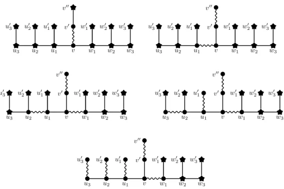
Figure 1: The 3-choice gadget H, and the way the initial matching M = {vv0} is being (= 3)-augmented until a matching of size µ=3(H, M ) is attained (from top to bottom, and left to right). Star vertices are exposed vertices. Wiggly edges are edges of the matching.
3. Augmenting matchings via (= k)-augmentations
We now investigate the consequences, on M P≤k, of restricting ourselves to augmentations of paths with length exactly k. In Section 3.1, we start by showing that M P=k is, in general, NP-hard for every k ≥ 3. The case of trees is considered in Section 3.2, wherein we prove that, in this context, the problem is NP-hard when k is part of the instance.
3.1. Complexity of M P=k in general graphs (for fixed k)
First, we would like to point out that, in the reduction of [NSW15] for showing that M P≤k is NP-hard for every k ≥ 5, only (= k)-augmentations can actually be performed in the reduced graphs, which can be checked by considering the pairs of exposed vertices. Therefore, from this reduction we directly get the following.
Theorem 3.1. [NSW15] M P=k is NP-hard for every k ≥ 5, even when restricted to instances
where G is a planar bipartite graph with maximum degree 3.
Since M P≤3was shown to be polynomial-time solvable [NSW15], we do not get the NP-hardness of M P=3 right away, in a similar way, and instead have to provide a proof.
Theorem 3.2. M P=3 is NP-hard, even when restricted to instances where G is a planar bipartite graph with maximum degree 3 and arbitrarily large girth.
Before going to the proof of Theorem 3.2, we first describe the gadgets to be used, as well as some of their behaviours. We start off with choice gadgets (see Figure 1 for an illustration). For any ` ≥ 2, the `-choice gadget is obtained from a path (u`, u`−1, · · · , u1, v, w1, · · · , w`−1, w`) on 2` + 1 vertices by 1) joining a new pendant vertex u0i to ui, for every i = 1, · · · , `, 2) joining a new pendant vertex w0ito wi, for every i = 1, · · · , `, then 3) joining a new pendant vertex v0 to v, and 4) joining a new pendant vertex v00 to v0. We call vv0 the middle-edge of the choice gadget. Throughout this section, assuming it is clear which choice gadget we are dealing with, we refer to its vertices and edges using the terminology we have just introduced.
Observation 3.3. Let H be an `-choice gadget, and M = {vv0} be a matching of H. Then, for any matching M0 of size µ=3(H, M ) obtained by performing (= 3)-augmentations starting from M , we have either: 1. M0 = {v0v00} ∪ {vw1} ∪S`i=1{uiu0i}, or 2. M0 = {v0v00} ∪ {vu1} ∪S ` i=1{wiwi0}. In particular, we have µ=3(H, M ) = ` + 2.
Proof. Consider a maximum sequence S = (P1, · · · , Pq) of (= 3)-augmentations that can be
per-formed starting from M , and denote by M0 the resulting matching. Throughout this proof, for
every 1 ≤ i ≤ q, we denote by S(M, i) the matching obtained from M by augmenting sequentially the paths P1, · · · , Pi. Note that S(M, q) = M0.
Recall that a (= 3)-augmentation can only be performed on a path of length 3 in which only the middle-edge belongs to the matching. For this reason, since M = {vv0}, we have P1= (v00, v0, v, u1)
or P1 = (v00, v0, v, w1). Assume P1 = (v00, v0, v, u1) without loss of generality (the other case is symmetric). Because v00v0 ∈ S(M, 1) and v00has degree 1, no augmenting path can contain any of v00and v0. So P2necessarily contains w1v and vu1. More precisely, P2may be either (w1, v, u1, u2) or (w1, v, u1, u01). At this point, it can be noted that, since vw1 and vu1 belong to one of P1 and P2, they cannot belong to any Pi with i ≥ 3. Indeed, whatever be the choice of P2, after its augmentation, all the neighbours of v get covered, and, thus, no edge incident to v may belong to an augmenting path of length 3 from this point. This implies that none of w2 and w01 belongs to one of the Pi’s, thus that the matching cannot be spread further towards the wi’s. We also note that if P2= (w1, v, u1, u01), then, in H and S(M, 2), there is no further (= 3)-augmentation, which means that the matching cannot propagate further towards the ui’s. So we necessarily have P2= (w1, v, u1, u2).
We thus have S(M, 2) = {v0v00, vw1, u1u2}, and the only augmenting (= 3)-paths are (u01, u1, u2, u02) and (u01, u1, u2, u3) (if ` ≥ 3). If ` = 2, then necessarily P3= (u01, u1, u2, u02), and we are done. If ` > 3, we note that P3 cannot be (u01, u1, u2, u02) as otherwise S(M, 3) would have no augment-ing (= 3)-paths in H. So, in that case, P3 = (u01, u1, u2, u3). These arguments generalize as follows by induction on i (see Figure 1 for an illustration). For every i = 2, · · · , ` + 1, the only (= 3)-augmenting paths in H, assuming the current matching is S(M, i − 1), are (u0i−1, ui−1, ui, u0i) and (u0i−1, ui−1, ui, ui+1). In case i = ` + 1, actually only the first of these two paths exists, so Pi = (u0i−1, ui−1, ui, u0i). Otherwise, i.e., i = 2, · · · , `, we note that having Pi= (u0i−1, ui−1, ui, u0i) would make S(M, i) have no augmenting (= 3)-paths in H. So we have Pi= (u0i−1, ui−1, ui, ui+1) for every i = 2, · · · , `, so that the matching can be spread further.
Under the assumption that P1= (v00, v0, v, u1), we eventually get, assuming that S is maximum, that M0 = {v0v00} ∪ {vw1} ∪S
`
i=1{uiu0i}. By symmetry, we note that having P1 = (v00, v0, v, w1) results in M0 = {v0v00} ∪ {vu
1} ∪S `
i=1{wiwi0}. In both cases, we have µ=3(H, M ) = ` + 2, as claimed.
In order to introduce the next type of gadgets, we need some additional terminology to deal with choice gadgets. Let H be a choice gadget. The vertices u0i of H are called the spike vertices of H, while the edges uiu0i incident to the spike vertices are called the spike edges. Each spike vertex or edge is numbered accordingly to the index i of the vertex u0i (or w0i) it intersects. The vertices u1, u01, u2, u02, · · · form the positive branch of H, while the vertices w1, w01, w2, w20, · · · form the negative branch. Rephrased differently, Observation 3.3 says that, in a choice gadget, the “optimal” way to propagate the original matching is towards the spike edges of the positive branch only, or towards the spike edges of the negative branch only. In the first case, we say that the original matching has been propagated positively, while we say it has been propagated negatively otherwise.
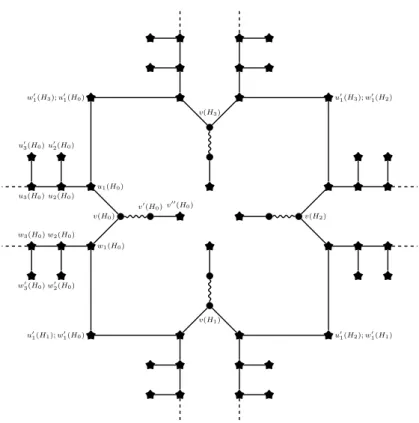
We now introduce variable gadgets, that are combinations of choice gadgets connected in a cyclic fashion (see Figure 2 for an illustration). For any m ≥ 1, the m-variable gadget is constructed as follows. The 1-variable gadget is the `-choice gadget (the length ` of the choice gadget will be fixed later). Then, for any m ≥ 2, the m-variable gadget is constructed by taking m `-choice gadgets H0, · · · , H`−1 and, for every i = 0, · · · , ` − 1, by identifying the first negative spike vertex of Hi
v(H3) w0 1(H3); u01(H0) u01(H3); w01(H2) v00(H 0) v0(H 0) v(H0) w1(H0) u1(H0) w2(H0) u2(H0) w3(H0) u3(H0) w0 2(H0) u0 2(H0) w0 3(H0) u0 3(H0) v(H1) u0 1(H2); w0 1(H1) u0 1(H1); w0 1(H0) v(H2)
Figure 2: The 4-variable gadget. Star vertices are exposed vertices. Wiggly edges are edges of the matching.
and the first positive spike vertex of Hi+1, where the indexes are understood modulo m. Precisely, for any j < m and any i ≤ `, let, here and further, ui(Hj) denote the vertex ui of the jth copy Hj of the choice gadget (v(Hj), v0(Hj), v00(Hj), u0i(Hj), wi(Hj), w0i(Hj) are defined analogously). Hence, the variable gadget is obtained by identifying w01(Hj) with u01(Hj+1) (modulo m) for every j = 0, · · · , m − 1.
The original matching of any variable gadget is the union of the original matchings of the choice gadgets constituting it (i.e., their middle-edges). By the positive branches (resp. negative branches) of H, we mean the m positive (resp. negative) branches of its underlying choice gadgets. Analogously, by referring to the spike vertices and spike edges of a variable gadget, we mean the spike vertices and edges of its underlying choice gadgets.
Note that we have not explicited the lengths of the 2m branches composing an m-variable gadget, i.e., ` still must be defined. However, we must now ensure that the behaviour described in Observation 3.3 remains valid after having combined the choice gadgets to form a variable gadget. Assuming these branches are “long enough”, we prove it is the case.
Observation 3.4. Let H be an m-variable gadget, and M be the original matching of H as described above. If ` (the length of the choice gadgets composing H) is at least 2, then, for any matching M0 of size µ=3(H, M ) obtained by performing (= 3)-augmentations starting from M , we have either:
1. all positive spike edges in M0 and no negative spike edges in M0, or 2. all negative spike edges in M0 and no positive spike edges in M0.
Proof. Let H0, · · · , Hm−1be the m `-choice gadgets composing H. We first prove that, because ` ≥ 2, any maximum sequence of (= 3)-augmentations has no interest to perform (= 3)-augmentations that intersect different choice gadgets. That is, a matching of size µ=3(H, M ) cannot be obtained by augmenting a (= 3)-path having edges in two consecutive Hi’s.
For purpose of contradiction, let us assume that there is an augmenting (= 3)-path Q that intersects two choice gadgets, w.l.o.g., say H0 and H1 and that Q has two edges in H0. Let us
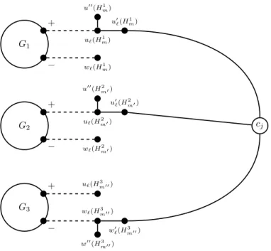
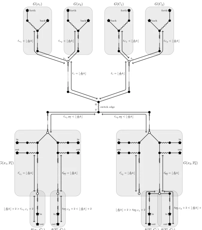
G1 + − u`(H1m) w`(Hm1) u00(H1 m) u0 `(H 1 m) G2 + − u`(Hm02 ) w`(H2m0) u00(H2 m0) u0 `(H 2 m0) G3 + − u`(Hm003 ) w`(Hm003 ) w00(H3 m00) w0 `(H 3 m00) cj
Figure 3: Illustration of the reduction in the proof of Theorem 3.2, for a formula Φ having a clause C = (x1∨x2∨x3), and C is the mth(resp. m0th, m00th) clause containing x
1(resp. x2, x3).
assume that Q is the first (to be augmented) such path intersecting distinct choice gadgets. When Q is about to be augmented, w1(H0)w10(H0) must be in the current matching, a neighbour of w1(H0) must be exposed, and u1(H1) must be exposed. The only way to have reached such a situation is when, in H0, the paths (v00(H0), v0(H0), v(H0), w1(H0)) and (u1(H0), v(H0), w1(H0), w10(H0)) have been augmented, and only them. Moreover, only the path (v00(H1), v0(H1), v(H1), w1(H1)) can have been augmented in H1.
Therefore, Q must be (w2(H0), w1(H0), w10(H0), u1(H1)). After having augmented Q, we note that, because all of v00(H0), v0(H0), v(H0), u1(H0), w1(H0)w2(H0), w10(H0) are covered, there is, in H, no further (= 3)-augmentation including an edge of H0. In H1, we note that, since u01(H1) and u1(H1) are covered, the only (= 3)-augmentation that can potentially be performed (if not already) in H1 is (v00(H1), v0(H1), v(H1), w1(H1)). According to these arguments, augmenting a (= 3)-path intersecting H0 and H1 leads to a final matching with at most three edges in H0 and
three edges in H1, while by Observation 3.3 we could have achieved a matching with ` + 2 ≥ 4
edges in each of H0 and H1 by propagating the matching positively or negatively.
Following these observations, since ` ≥ 2, a matching of size µ=3(H, M ) can only be obtained, from M , by propagating the original matching of each Hi positively or negatively. The claim now follows from the fact that if, say, Hi has propagated its matching negatively, then Hi+1 cannot propagate its matching positively, since the first negative spike edge of Hi and the first positive spike edge of Hi+1 are adjacent.
According to Observation 3.4, we can thus derive the notion of positive and negative prop-agations to variable gadgets with long branches: by propagating its matching positively (resp. negatively), we mean propagating the matching positively (resp. negatively) in all of its underlying choice gadgets.
We now have all ingredients in hand for proving Theorem 3.2.
Proof of Theorem 3.2. The proof is by reduction from 3-SAT. Namely, from a 3CNF formula Φ, we construct, in polynomial time, a graph G with an initial matching M such that, from a satisfiable truth assignment of the variables of Φ, we can deduce a matching of size µ=3(G, M ) to which M can be (= 3)-augmented, and vice versa.