HAL Id: hal-00680634
https://hal-paris1.archives-ouvertes.fr/hal-00680634
Submitted on 27 Mar 2012
HAL is a multi-disciplinary open access archive for the deposit and dissemination of sci-entific research documents, whether they are pub-lished or not. The documents may come from teaching and research institutions in France or abroad, or from public or private research centers.
L’archive ouverte pluridisciplinaire HAL, est destinée au dépôt et à la diffusion de documents scientifiques de niveau recherche, publiés ou non, émanant des établissements d’enseignement et de recherche français ou étrangers, des laboratoires publics ou privés.
Endogenous Entry, Product Variety and Business Cycles
Florin Bilbiie, Fabio Ghironi, Marc Melitz
To cite this version:
Florin Bilbiie, Fabio Ghironi, Marc Melitz. Endogenous Entry, Product Variety and Business Cycles. Journal of Political Economy, University of Chicago Press, 2012, 120 (2), pp.304-345. �10.1086/665825�. �hal-00680634�
Endogenous Entry, Product Variety, and Business Cycles
Florin O. Bilbiiey
Paris School of Economics, Université Paris 1 Panthéon-Sorbonne,
and CEPR
Fabio Ghironiz
Boston College,
Federal Reserve Bank of Boston, EABCN, and NBER
Marc J. Melitzx
Harvard University, CEPR, and NBER
March 12, 2012
Previously circulated under the title “Business Cycles and Firm Dynamics” and …rst presented in the summer of 2004. For helpful comments, we thank Robert Shimer, two anonymous referees, Susanto Basu, Christian Broda, Sanjay Chugh, Andrea Colciago, Diego Comin, Fiorella De Fiore, Massimo Giovannini, Jean-Olivier Hairault, Robert Hall, Kólver Hernández, Boyan Jovanovic, Nobuhiro Kiyotaki, Oleksiy Kryvtsov, Philippe Martin, Kris Mitchener, José-Víctor Ríos-Rull, Nicholas Sim, Viktors Stebunovs, Michael Woodford, and participants in many conferences and seminars. We are grateful to Brent Bundick, Massimo Giovannini, Nicholas Sim, Viktors Stebunovs, and Pinar Uysal for excellent research assistance. Remaining errors are our responsibility. Bilbiie thanks the NBER, the CEP at LSE, and the ECB for hospitality in the fall of 2006, 2005, and summer of 2004, respectively; Nu¢eld College at Oxford for …nancial support during the 2004-2007 period; and Banque de France for …nancial support through the Chaire Banque de France at the Paris School of Economics. Ghironi and Melitz thank the NSF for …nancial support through a grant to the NBER. The views expressed in this paper are those of the authors and do not necessarily re‡ect those of Banque de France, the Federal Reserve Bank of Boston or Federal Reserve policy.
yCentre d’Economie de la Sorbonne, 106-112 Boulevard de l’Hôpital, Paris 75013, France. E-mail:
‡[email protected]. URL: http://‡orin.bilbiie.googlepages.com.
zDepartment of Economics, Boston College, 140 Commonwealth Avenue, Chestnut Hill, MA 02467-3859, U.S.A.
E-mail: [email protected]. URL: http://fmwww.bc.edu/ec/Ghironi.php.
xDepartment of Economics, Harvard University, Littauer Center, 1805 Cambridge Street, Cambridge, MA 02138,
Abstract
This paper builds a framework for the analysis of macroeconomic ‡uctuations that incorpo-rates the endogenous determination of the number of producers and products over the business cycle. Economic expansions induce higher entry rates by prospective entrants subject to irre-versible investment costs. The sluggish response of the number of producers (due to sunk entry costs and a time-to-build lag) generates a new and potentially important endogenous propaga-tion mechanism for real business cycle models. The return to investment (corresponding to the creation of new productive units) determines household saving decisions, producer entry, and the allocation of labor across sectors. The model performs at least as well as the benchmark real business cycle model with respect to the implied second-moment properties of key macroeco-nomic aggregates. In addition, our framework jointly predicts procyclical product variety and procyclical pro…ts even for preference speci…cations that imply countercyclical markups. When we include physical capital, the model can simultaneously reproduce most of the variance of GDP, hours worked, and total investment found in the data.
1 Introduction
This paper studies the role of endogenous producer entry and creation of new products in propa-gating business cycle ‡uctuations. Towards that goal, we develop a dynamic, stochastic, general equilibrium (DSGE) model with monopolistic competition, consumer love for variety, and sunk entry costs. We seek to understand the contributions of the intensive and extensive margins – changes in production of existing goods and in the range of available goods – to the response of the economy to changes in aggregate productivity.
Empirically, new products are not only introduced by new …rms, but also by existing …rms (most often at their existing production facilities). We therefore take a broad view of producer entry (and exit) as also incorporating product creation (and destruction) by existing …rms, although our model does not address the determinants of product variety within …rms. Even though new …rms account for a small share of overall production (for U.S. manufacturing, new …rms account for 2-3% of both overall production and employment), the contribution of new products (including those produced at existing …rms) is substantially larger – important enough to be a major source of aggregate output changes. Furthermore, as is the case with …rm entry, new product creation is also very strongly procyclical.1
The important contribution of product creation and destruction to aggregate output is convinc-ingly documented in a recent paper by Bernard, Redding, and Schott (2010), who are the …rst to measure product creation and destruction within …rms across a large portion of the U.S. economy (all U.S. manufacturing …rms). For each …rm, they record production levels (dollar values) across 5-digit U.S. SIC categories, which still represent a very coarse de…nition of products.2 Bernard, Redding, and Schott …rst document that 94% of product additions by U.S. manufacturing …rms occur within their pre-existing production facilities (as opposed to new plants or via mergers and acquisitions). They further show that 68% of …rms change their product mix within a 5-year census period (representing 93% of …rms weighted by output). Of these …rms, 66% both add and drop
1The working paper version of this study (Bilbiie, Ghironi, and Melitz, 2007) contains evidence on the procyclicality
of net …rm entry (measured as new incorporations minus failures) and pro…ts for the period 1947-1998. Our conclusions there are in line with the pioneering work of Dunne, Roberts and Samuelson (1988). Here, we focus on product creation, rather than …rm entry.
2As an example, the 5-digit SIC codes within the 4-digit SIC category 3949–Sporting and Athletics Goods– are:
39491–Fishing tackle and equipment, 39492–Golf equipment, 39493–Playground equipment, 39494–Gymnasium and exercise equipment, and 39495–Other sporting and athletic goods. For all of U.S. manufacturing, there are 1848 5-digit products.
products (representing 87% of …rms weighted by output). Thus, product creation over time is not just a secular trend at the …rm level (whereby …rms steadily increase the range of products they produce over time). Most importantly, Bernard, Redding, and Schott show that product creation and destruction account for important shares of overall production: Over a 5-year period – a hori-zon usually associated with the length of business cycles –, the value of new products (produced at existing …rms) is 33.6% of overall output during that period (-30.4% of output for the lost value from product destruction at existing …rms). These numbers are almost twice (1.8 times) as large as those accounted for by changes at the intensive margin – production increases and decreases for the same product at existing …rms. The overall contribution of the extensive margin (product creation and destruction) would be even higher if a …ner level of product disaggregation (beyond the 5-digit level) were available.3
Put together, product creation (both by existing …rms and new …rms) accounts for 46.6% of output in a 5-year period, while the lost value from product destruction (by existing and exiting …rms) accounts for 44% of output. This represents a minimal annual contribution of 9.3% (for product creation) and 8.8% (for product destruction). The actual annual contributions are likely larger, not only because the coarse de…nition of a product potentially misses much product creation and destruction within the 5-digit SIC category, but also because additions to and subtractions from output across years within the same 5-year interval (for a given …rm-product combination) are not recorded. Relatedly, Den Haan and Sedlacek (2010) estimate the contribution of the extensive margin (measured along the employment dimension) to total value added. They calculate the contribution of ’cyclical workers’ (workers who during the period under scrutiny experienced a non-employment spell) over a 3-year interval for Germany and the U.S. and …nd that this amounts to roughly half of total value added.
The substantial contribution of product creation and destruction is also con…rmed by Broda and Weinstein (2010), who measure products at the …nest possible level of disaggregation: the product barcode. Their data cover all of the purchases of products with barcodes by a representative sample of U.S. consumers. An important feature of the evidence in Bernard, Redding, and Schott (2010)
3Returning to the example of 5-digit SIC 39494 (Gymnasium and exercise equipment) from the previous footnote:
Any production of a new equipment product, whether a treadmill, an elliptical machine, a stationary bike, or any weight machine, would be recorded as production of the same product and hence be counted toward the intensive margin of production.
is con…rmed by Broda and Weinstein’s highly disaggregated data: 92% of product creation occurs within existing …rms. Broda and Weinstein …nd that 9% of the consumers’ purchases in a year are devoted to new goods not previously available.4 Similarly to Bernard, Redding, and Schott (2010), Broda and Weinstein …nd that the market share of new products is four times larger than the market share of new …rms (measured either in terms of output or employment), precisely because most product creation occurs within the …rm (the same conclusion arises for product destruction versus …rm exit). Furthermore, Broda and Weinstein report that this product creation is strongly procyclical at quarterly business cycle frequency. The evidence on the strong procyclicality of product creation is also con…rmed by Axarloglou (2003) for U.S. manufacturing at a monthly frequency.
In our model, we assume symmetric, homothetic preferences over a continuum of goods. This nests several tractable speci…cations (including C.E.S.) as special cases. To keep the setup simple, we do not model multi-product …rms. In our model presentation below, and in the discussion of results, there is a one-to-one identi…cation between a producer, a product, and a …rm. This is consistent with much of the macroeconomic literature with monopolistic competition, which similarly uses “…rm” to refer to the producer of an individual good. However, the relevant pro…t-maximizing unit in our setup is best interpreted as a production line, which could be nested within a multi-product …rm. The boundary of the …rm across products is then not determined. Strategic interactions (within and across …rms) do not arise due to our assumption of a continuum of goods, so long as each multi-product …rm produces a countable set of goods of measure zero.5 In this interpretation of our model, producer entry and exit capture the product-switching dynamics within …rms documented by Bernard, Redding, and Schott (2010).
In our baseline setup, each individual producer/…rm produces output using only labor. However, the number of …rms that produce in each period can be interpreted as the capital stock of the economy, and the decision of households to …nance entry of new …rms is akin to the decision to
4This 9% …gure is low relative to its 9.3% counterpart from Bernard, Redding, and Schott (2010), given the
substantial di¤erence in product disaggregation across the two studies (the extent of product creation increases monotonically with the level of product disaggregation). We surmise that this is due to the product sampling of Broda and Weinstein’s (2010) data: only including …nal goods with barcodes. Food items, which have the lowest levels of product creation rates, tend to be over-represented in those samples.
5This di¤erentiates our approach from Jaimovich and Floetotto (2008), who assume a discrete set of producers
within each sector. In that case, the boundaries of …rms crucially determine the strategic interaction between individual competitors.
accumulate physical capital in the standard real business cycle (RBC) model. Product creation (or, more broadly, entry) takes place subject to sunk product development costs, which are paid by investors in the expectation of future pro…ts. Free entry equates the value of a product (the present discounted value of pro…ts) to the sunk cost; subsequent to entry, the per-period pro…ts ‡uctuate endogenously. This distinguishes our framework from earlier studies that modeled entry in a frictionless way: there, entry drives pro…ts to zero in every period. (We discuss the relation between our work and these studies later on.) Our framework is hence closer to that of variety-based endogenous growth models (see e.g. Romer, 1990, Grossman and Helpman, 1991, and Aghion and Howitt, 1991). Indeed, just as the RBC model is a discrete-time, stochastic, general equilibrium version of the exogenous growth model that abstracts from growth to focus on business cycles, our model can be viewed as a discrete-time, stochastic, general equilibrium version of variety-based, endogenous growth models that abstracts from endogenous growth (We discuss in greater detail further on why we have chosen to abstract from growth).
From a conceptual standpoint, linking innovation-based growth and business cycle theory is not new: The history of this idea goes back at least to Schumpeter (1934). Aghion and Howitt (1991) review some attempts at unifying growth and business cycles. Shleifer’s (1986) theory of implementation cycles is one example of the conceptual link between (endogenous) business cycles and innovation-based growth theory: cycles occur because …rms, expecting higher pro…ts in booms due to a demand externality, innovate simultaneously in the expectation of a boom; the boom therefore becomes self-ful…lling. However, to the best of our knowledge this is the …rst study that blends elements of variety-based endogenous growth theory and RBC methodology (including the focus on exogenous aggregate productivity as the only source of uncertainty). Moreover, our framework also uses a general structure of preferences for variety that implies that markups fall when market size increases (which can be viewed as a dynamic extension of Krugman’s, 1979 insights about the e¤ects of market size on …rm size and markups).
The investment in new productive units is …nanced by households through the accumulation of shares in the portfolio of …rms. The stock-market price of this investment ‡uctuates endogenously in response to shocks and is at the core of our propagation mechanism. Together with the shares’ payo¤ (monopolistic pro…ts), it determines the return to investment/entry, which in turn determines household saving decisions, producer entry, and the allocation of labor across sectors in the economy.
This contrasts with the standard, one-sector RBC models, where the price of physical capital is constant absent capital adjustment costs, and the return to investment is simply equal to the marginal product of physical capital. This approach to investment and the price of capital provides an alternative to adjustment costs in order to obtain a time-varying price of capital. It also introduces a direct link between investment and (the expectation of) economic pro…ts. In our model, labor is allocated to production of existing goods and creation of new ones; and the total number of products acts as capital in the production of the consumption basket. This structure is close to two-sector versions of the RBC model where labor is allocated to production of the consumption good and to investment that augments the capital stock; and capital is also used to produce the consumption good. We discuss this relationship in further detail below.
In terms of matching key second moments of the U.S. business cycle, our baseline model per-forms at least as well as a traditional RBC model (it does better at matching the volatility of output and hours). Importantly, our model can additionally account for stylized facts pertaining to entry, pro…ts, and markups. With translog preferences (for which the elasticity of substitution is increasing in the number of goods produced), our model is further able to simultaneously generate countercyclical markups and procyclical pro…ts; it also reproduces the time pro…le of the markup’s correlation with the business cycle. These are well-known challenges for models of countercyclical markups based on sticky prices (see Rotemberg and Woodford, 1999, for a discussion). To the best of our knowledge, our framework is the …rst to address and explain these issues simultaneously.6 Moreover, we develop an extension of our framework that also incorporates investment in physical capital. This signi…cantly improves the performance of the model (relative to both our baseline without physical capital and the standard RBC model) in reproducing the volatilities of output, hours worked, and total investment.
The structure of the paper is as follows. Section 2 presents the baseline model. Section 3 computes impulse responses and second moments for a numerical example and illustrates the prop-erties of the model for transmission of economic ‡uctuations. Section 4 outlines the extension of our model to include investment in physical capital and illustrates its second-moment properties.
6Perfect-competition models, such as the standard RBC, address none of these facts. Imperfect-competition
versions (with or without sticky prices) generate ‡uctuations in pro…ts (and, for sticky prices, in markups) but no entry. Frictionless-entry models discussed later generate ‡uctuations in entry (and, in some versions – such as Cook, 2001, Comin and Gertler, 2006, or Jaimovich and Floetotto, 2008 –, also markups) but with zero pro…ts.
Section 5 discusses the relation between our work and other contributions to the literature on entry and business cycles. Section 6 concludes.
2 The Model
2.1 Household Preferences and the Intratemporal Consumption Choice
The economy is populated by a unit mass of atomistic, identical households. All contracts and prices are written in nominal terms. Prices are ‡exible. Thus, we only solve for the real variables in the model. However, as the composition of the consumption basket changes over time due to …rm entry (a¤ecting the de…nition of the consumption-based price index), we introduce money as a convenient unit of account for contracts. Money plays no other role in the economy. For this reason, we do not model the demand for cash currency, and resort to a cashless economy as in Woodford (2003).
The representative household supplies Lthours of work each period t in a competitive labor
mar-ket for the nominal wage rate Wtand maximizes expected intertemporal utility Et P1s=t s tU (Cs; Ls) ,
where C is consumption and 2 (0; 1) the subjective discount factor. The period utility function takes the form U (Ct; Lt) = ln Ct (Lt)1+1='= (1 + 1='), > 0, where ' 0 is the Frisch
elas-ticity of labor supply to wages, and the intertemporal elaselas-ticity of substitution in labor supply. Our choice of functional form for the utility function is guided by results in King, Plosser, and Rebelo (1988): Given separable preferences, log utility from consumption ensures that income and substitution e¤ects of real wage variation on e¤ort cancel out in steady state; this is necessary to have constant steady-state e¤ort and balanced growth if there is productivity growth.
At time t, the household consumes the basket of goods Ct, de…ned over a continuum of goods
. At any given time t, only a subset of goods t is available. Let pt(!) denote the nominal
price of a good ! 2 t. Our model can be solved for any parametrization of symmetric homothetic
preferences. For any such preferences, there exists a well de…ned consumption index Ct and an
associated welfare-based price index Pt. The demand for an individual variety, ct(!), is then
obtained as ct(!)d! = Ct@Pt=@pt(!), where we use the conventional notation for quantities with a
continuum of goods as ‡ow values (see the Appendix for more details).
symmetric price elasticity of demand is in general a function of the number Ntof goods (where Nt
is the mass of t): (Nt) (@ct(!)=@pt(!)) (pt(!)=ct(!)), for any symmetric variety !. The bene…t
of additional product variety is described by the relative price t(!) = (Nt) pt(!)=Pt, for any
symmetric variety !, or, in elasticity form: (Nt) 0(Nt)Nt= (Nt). Together, (Nt) and (Nt)
completely characterize the e¤ects of consumption preferences in our model; explicit expressions for these objects can be obtained upon specifying functional forms for preferences, as will become clear in the discussion below.
2.2 Firms
There is a continuum of monopolistically competitive …rms, each producing a di¤erent variety ! 2 . Production requires only one factor, labor (this assumption is relaxed in Section 4, where we introduce physical capital). Aggregate labor productivity is indexed by Zt, which represents the
e¤ectiveness of one unit of labor. Zt is exogenous and follows an AR(1) process (in logarithms).
Output supplied by …rm ! is yt(!) = Ztlt(!), where lt(!) is the …rm’s labor demand for productive
purposes. The unit cost of production, in units of the consumption basket Ct, is wt=Zt, where
wt Wt=Pt is the real wage.
Prior to entry, …rms face an exogenous sunk entry cost of fE e¤ective labor units (as in Grossman
and Helpman, 1991, Judd, 1985, and Romer, 1990, among others), equal to wtfE=Zt units of
the consumption basket. This speci…cation ensures that exogenous productivity shocks are truly aggregate in our model, as they a¤ect symmetrically both production of existing goods and creation of new products.7 Given our modeling assumption relating each …rm to a product line, we think
of the entry cost as the development and setup cost associated with a particular variety.
There are no …xed production costs. Hence, all …rms that enter the economy produce in every period, until they are hit with a “death” shock, which occurs with probability 2 (0; 1) in every period. The assumption of exogenous exit is adopted here only in the interest of tractability. Recent evidence suggests that this assumption is a reasonable starting point for analysis. At the product level, Broda and Weinstein (2010) report that product destruction is much less cyclical than product creation. A similar pattern also holds at the plant level; using U.S. Census (annual) data, Lee and Mukoyama’s (2007) …nd that, while plant entry is highly procyclical (the entry rate
7Thus, the “production function” for new goods is N
is 8.1 percent in booms and 3.4 percent in recessions), annual exit rates are similar across booms and recessions (5.8 and 5.1 percent, respectively). They also …nd that plants exiting in recessions are very similar to those exiting in booms (in terms of employment or productivity).
In units of consumption, variety !’s price will be set to t(!) pt(!) =Pt= twt=Zt, where t
is the price markup over marginal cost (anticipating symmetric equilibrium). Given our demand speci…cation with endogenous price elasticity of residual demand, this markup is a function of the number of producers: t = (Nt) (Nt)= ( (Nt) + 1) : The pro…ts generated from the sales of
each variety (expressed in units of consumption) are dt(!) = dt = 1 (Nt) 1 Ct=Nt and are
returned to households as dividends.
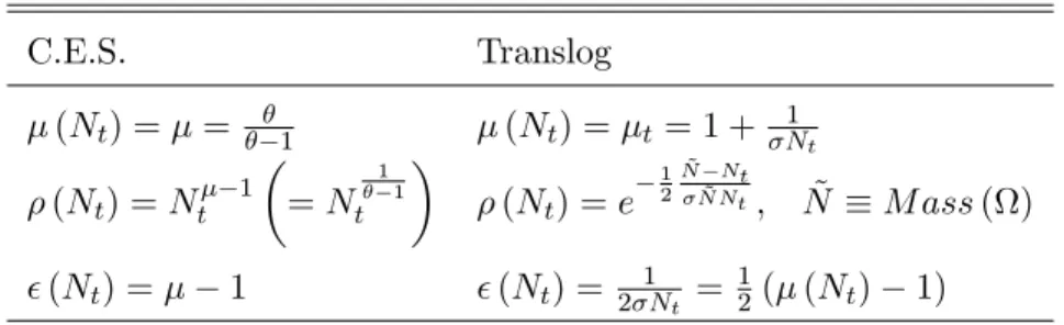
2.2.1 Preference Speci…cations and Markups
In our quantitative exercises, we consider two alternative speci…cations that are nested within our general analysis of symmetric homothetic preferences. The …rst speci…cation features con-stant elasticity of substitution between goods as in Dixit and Stiglitz (1977). For these C.E.S. preferences, the consumption aggregator is Ct = R!2 ct(!) 1= d!
=( 1)
; where > 1 is the symmetric elasticity of substitution across goods. The consumption-based price index is then Pt = R!2 tpt(!)1 d!
1=(1 )
; and the household’s demand for each individual good ! is ct(!) = (pt(!) =Pt) Ct. It follows that the markup and the bene…t of variety are independent
of the number of goods ( (Nt) = ; (Nt) = ) and related by = 1 = 1= ( 1) : The second
speci…cation uses the translog expenditure function proposed by Feenstra (2003), which introduces demand-side pricing complementarities. For this preference speci…cation, the symmetric price elas-ticity of demand is (1 + Nt), > 0: As Nt increases, goods become closer substitutes, and the
elasticity of substitution 1 + Nt increases. If goods are closer substitutes, then the markup (Nt)
and the bene…t of additional varieties in elasticity form ( (Nt)) must decrease. This property
occurs whenever the price elasticity of residual demand decreases with quantity consumed along the residual demand curve. The change in (Nt) is only half the change in net markup generated
by an increase in the number of producers. Table 1 contains the expressions for markup, relative price, and the bene…t of variety (the elasticity of to the number of …rms), for each preference speci…cation.
2.2.2 Firm Entry and Exit
In every period, there is a mass Nt of …rms producing in the economy and an unbounded mass of
prospective entrants. These entrants are forward looking, and correctly anticipate their expected future pro…ts ds(!) in every period s t + 1 as well as the probability (in every period) of
incurring the exogenous exit-inducing shock. Entrants at time t only start producing at time t + 1, which introduces a one-period time-to-build lag in the model. The exogenous exit shock occurs at the very end of the time period (after production and entry). A proportion of new entrants will therefore never produce. Prospective entrants in period t compute their expected post-entry value (vt(!)) given by the present discounted value of their expected stream of pro…ts fds(!)g1s=t+1:
vt(!) = Et 1
X
s=t+1
Qt;sds(!) ; (1)
where Qt;s is the stochastic discount factor that is determined in equilibrium by the optimal
invest-ment behavior of households. This also represents the value of incumbent …rms after production has occurred (since both new entrants and incumbents then face the same probability 1 of survival and production in the subsequent period). Entry occurs until …rm value is equalized with the entry cost, leading to the free entry condition vt(!) = wtfE=Zt. This condition holds so long as the mass
NE;t of entrants is positive. We assume that macroeconomic shocks are small enough for this
con-dition to hold in every period. Finally, the timing of entry and production we have assumed implies that the number of producing …rms during period t is given by Nt= (1 ) (Nt 1+ NE;t 1). The
number of producing …rms represents the stock of capital of the economy. It is an endogenous state variable that behaves much like physical capital in the benchmark RBC model, but in contrast to the latter has an endogenously ‡uctuating price given by (1).
2.2.3 Symmetric Firm Equilibrium
All …rms face the same marginal cost. Hence, equilibrium prices, quantities, and …rm values are identical across …rms: pt(!) = pt, t(!) = t, lt(!) = lt, yt(!) = yt, dt(!) = dt, vt(!) = vt.
In turn, equality of prices across …rms implies that the consumption-based price index Pt and the
…rm-level price pt are such that pt=Pt t = (Nt). An increase in the number of …rms implies
necessarily that the relative price of each individual good increases, 0(N
more …rms, households derive more welfare from spending a given nominal amount, i.e., ceteris paribus, the price index decreases. It follows that the relative price of each individual good must rise. The aggregate consumption output of the economy is Nt tyt = Ct,which we can rewrite as
Ct = Zt (Nt) (Lt fENE;t=Zt). An increase in the number of entrants NE;t absorbs productive
resources and acts like an overhead labor cost in production of consumption. Importantly, in the symmetric …rm equilibrium, the option value of waiting to enter is zero, despite the presence of sunk costs and exit risk. This happens because all uncertainty in our model is aggregate, and the “death” shock is symmetric across …rms and time-invariant.8
2.3 Household Budget Constraint and Optimal Behavior
Households hold shares in a mutual fund of …rms. Let xt be the share in the mutual fund held by
the representative household entering period t. The mutual fund pays a total pro…t in each period (in units of currency) equal to the total pro…t of all …rms that produce in that period, PtNtdt.
During period t, the representative household buys xt+1 shares in a mutual fund of Nt+ NE;t…rms
(those already operating at time t and the new entrants). The mutual fund covers all …rms in the economy, even though only 1 of these …rms will produce and pay dividends at time t + 1. The date t price (in units of currency) of a claim to the future pro…t stream of the mutual fund of Nt+ NE;t …rms is equal to the nominal price of claims to future …rm pro…ts, Ptvt.
The household enters period t with mutual fund share holdings xt. It receives dividend income
on mutual fund share holdings, the value of selling its initial share position, and labor income. The household allocates these resources between purchases of shares to be carried into next period and consumption. The period budget constraint (in units of consumption) is:
vt(Nt+ NE;t) xt+1+ Ct= (dt+ vt) Ntxt+ wtLt: (2)
The household maximizes its expected intertemporal utility subject to (2). The Euler equations for share holdings is:
vt= (1 ) Et
Ct
Ct+1
(vt+1+ dt+1) :
8See the Appendix for the proof. This contrasts with i.a. Caballero and Hammour (1994) and Campbell (1998).
As expected, forward iteration of the equation for share holdings and absence of speculative bub-bles yield the asset price solution in equation (1), with the stochastic discount factor Qt;s =
[ (1 )]sCt=Ct+s.
Finally, the allocation of labor e¤ort obeys the standard intratemporal …rst-order condition:
(Lt)
1 ' = wt
Ct
: (3)
2.4 Aggregate Accounting, Labor Market Dynamics, and the Relation with RBC Theory
Di¤erent from the benchmark, one-sector, RBC model of Kydland and Prescott (1982) and many other studies, our model economy is a two-sector economy in which one sector employs part of the labor supply to produce consumption and the other sector employs the rest of the labor supply to produce new …rms. Labor market equilibrium requires that these two components of labor demand sum to aggregate labor supply: LCt + LEt = Lt, where LCt = Ntlt is the total amount of labor used
in production of consumption, and LEt = NE;tfE=Ztis labor used to create new …rms.
Aggregating the budget constraint (2) across households and imposing the equilibrium condition xt+1= xt= 1 8t yields the aggregate accounting identity for GDP Yt Ct+ NE;tvt= wtLt+ Ntdt.
Total consumption, Ct; plus investment (in new products or …rms) NE;tvt; must be equal to total
income (labor income wtLtplus dividend income Ntdt). Thus, vtis the relative price of the
invest-ment “good” in terms of consumption. In a one-sector RBC model, only the interest rate dictates the allocation of resources between consumption and investment. In our model, this allocation is re‡ected in the allocation of labor across the two sectors (producing consumption goods and new goods). The key distinction is that the relative price of investment vt‡uctuates and dictates the
al-location of labor across sectors, in conjunction with the return on shares, rE
t+1 (vt+1+ dt+1) =vt.
This is reminiscent of a two-sector RBC model9 where the relative price of investment is also
endogenous and a¤ects the allocation of resources to consumption versus investment.
Despite this similarity, there are important features that di¤erentiate our framework from a two-sector RBC structure: First, we model explicitly the microeconomic incentives for product creation from consumer love for variety and pro…t incentives for innovators; Second, we have a di¤erent
notion of investment, directed entirely toward the extensive margin (the creation of new goods), whereas all investment takes place at the intensive margin (machines used to produce more of the same good) in the RBC model (one-sector or two-sector). Both forms of investment take place in reality, and the version of our model introduced in Section 4 addresses this; Third, our model can address facts about entry, pro…ts, and markups. A two-sector RBC model that is otherwise isomorphic to ours would need the ad hoc assumption of a labor share in consumption output that is an appropriate function of capital to generate a procyclical labor share in GDP (as our model does under translog preferences); Fourth, since aggregate production of consumption in our model features a form of increasing returns due to variety, one needs to introduce increasing returns in the consumption sector of the RBC model to make it isomorphic to ours. But since internal increasing returns are inconsistent with perfect competition, one needs to adopt the ad hoc assumption of a labor externality in the consumption sector to avoid internal increasing returns at the …rm level (or otherwise assume that …rms price at average cost).10 For these reasons, and its traditional role as benchmark, we keep the one-sector RBC model as reference point for performance comparison below.
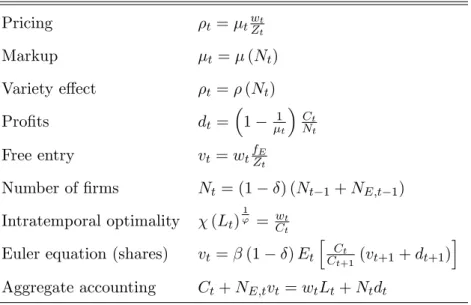
2.5 Model Summary
Table 2 summarizes the main equilibrium conditions of the model (the labor market equilibrium condition is redundant once the variety e¤ect equation is included). The equations in the table constitute a system of nine equations in nine endogenous variables: t; t; dt; wt; Lt; NE;t; Nt; vt;
Ct. Of these endogenous variables, one is predetermined as of time t: the total number of …rms,
Nt. Additionally, the model features one exogenous variable: aggregate productivity, Zt.
2.6 Steady State
We assume that productivity is constant in steady state and denote steady-state levels of variables by dropping the time subscript: Zt= Z. We conjecture that all endogenous variables are constant
in steady state and show that this is indeed the case. We de…ne the steady-state interest rate as a function of the rate of time preference, 1 + r 1. We exploit this below to treat r as a parameter
1 0Evidence in Harrison (2003) does not support the assumptions needed to make the models isomorphic. In
particular, Harrison …nds that returns to scale are slightly increasing in the investment sector, but they are decreasing or constant in the consumption sector.
in the solution. The full steady-state solution is presented in the Appendix. Here, we present the most important long-run properties of our model.
The gross return on shares is 1 + d=v = (1 + r)=(1 ), which captures a premium for expected …rm destruction. The number of new entrants makes up for the exogenous destruction of existing …rms: NE = N= (1 ). Calculating the shares of pro…t income and investment in consumption
output and GDP allows us to draw another transparent comparison between our model and the stan-dard RBC setup. The steady-state pro…t equation gives the share of pro…t income in consumption output: dN=C = ( 1) = . Using this result in conjunction with those obtained above, we have the share of investment in consumption output, denoted by : vNE=C = ( 1) = [ (r + )].
This expression is similar to its RBC counterpart. There, the share of investment in output is given by sK = (r + ) ; where is the depreciation rate of capital and sK is the share of capital
income in total income. In our framework, ( 1) = can be regarded as governing the share of “capital” since it dictates the degree of monopoly power and hence the share of pro…ts that …rms generate from producing consumption output (dN=C). Noting that Y = C+ vNE, the shares of
investment and pro…t income in GDP are vNE=Y = = (1 + ) and dN=Y = [(r + ) ] = [ (1 + )],
respectively. It follows that the share of consumption in GDP is C=Y = 1= (1 + ). The share of labor income in total income is wL=Y = 1 [(r + ) ] = [ (1 + )]. Importantly, all these ratios are constant. If we allowed for long-run growth (either via an exogenous trend in Zt, or endogenously
by assuming entry cost fE=Ntas in Grossman and Helpman, 1991), these long-run ratios would still
be constant with C.E.S. preferences, consistent with the Kaldorian growth facts. In fact, regardless of preference speci…cation within the homothetic class, our model’s long-run properties with growth would be consistent with two stylized facts originally found by Kaldor (1957): a constant share of pro…ts in total capital, dN=vN = (r + d)=(1 d), and, relatedly, a high correlation between the pro…t share in GDP and the investment share in GDP. These facts are absent from both the standard RBC model and the frictionless entry models discussed in Section 5.
We abstract from growth for two reasons (beyond the fact that it is the subject of its own extensive literature). In variety-based models, endogenous growth occurs whenever costs of product creation decrease with the number of existing products; in other words, the production function for new goods exhibits constant returns to scale in an accumulating factor, viz., the number of goods. The growth rate in such models (such as in the standard AK model) is a function of the level of
productivity: Any shock to productivity would immediately put the economy on the new balanced growth path with no transition dynamics. We focus instead on short-run ‡uctuations where the extensive margin does play a signi…cant role in propagating shocks. Second, the growth rate is also a function of the elasticity of substitution between goods, which is not constant (in general) in our model. Reconciling an endogenous time-varying markup with stylized growth facts (that imply constant markups and pro…t shares in the long run) is a challenge to growth theory that is worth future investigation but is beyond the scope of this paper.11
2.7 Dynamics
We solve for the dynamics in response to exogenous shocks by log-linearizing the model around the steady state. However, the model summary in Table 2 already allows us to draw some conclusions on the properties of shock responses for some key endogenous variables. It is immediate to verify that …rm value is such that vt = wtfE=Zt = fE (Nt) = (Nt). Since the number of producing …rms is
predetermined and does not react to exogenous shocks on impact, …rm value is predetermined with respect to productivity shocks. An increase in productivity results in a proportional increase in the real wage on impact through its e¤ect on labor demand. Since the entry cost is paid in e¤ective labor units, this does not a¤ect …rm value. An implication of the wage schedule wt= Zt (Nt) = (Nt) is
that also marginal cost, wt=Zt, is predetermined with respect to the shock.
We can reduce the system in Table 2 to a system of two equations in two variables, Nt and Ct
(see the Appendix). Using sans-serif fonts to denote percent deviations from steady-state levels, log-linearization around the steady state under assumptions of log-normality and homoskedasticity yields: Nt+1= 1 + r + 1 + r + 1 + ' ( ) Nt ' r + 1+ + r + 1 Ct (4) + (1 + ') r + 1 + Zt; Ct= 1 1 + rEtCt+1 1 1 + r( ) r + 1 + r 1 1 Nt+1+ ( ) Nt; (5)
where 0(N ) N= (N ) 0 is the elasticity of the markup function with respect to N;which takes
1 1Balanced growth would be restored under translog preferences by making the ad hoc assumption that the
the value of 0 under C.E.S and (1 + N ) 1 under translog preferences. Equation (4) states that the number of …rms producing at t + 1 increases if consumption at time t is lower (households save more in the form of new …rms) or if productivity is higher. Equation (5) states that consumption at time t is higher the higher expected future consumption and the larger the number of …rms producing at time t. The e¤ect of Nt+1 depends on parameter values. For realistic parameter
values, we have > (r + ) = (1 ): An increase in the number of …rms producing at t + 1 is associated with lower consumption at t. (Higher productivity at time t lowers contemporaneous consumption through this channel, as households save to …nance faster entry in a more attractive economy. However, we shall see below that the general equilibrium e¤ect of higher productivity will be that consumption rises.)
In the Appendix, we show that the system (4)-(5) has a unique, non-explosive solution for any possible parametrization. To solve the system, we assume Zt= ZZt 1+ "Z;t, where "Z;tis an i.i.d.,
Normal innovation with zero mean and variance "2Z.
3 Business Cycles: Propagation and Second Moments
In this section we explore the properties of our model by means of a numerical example. We compute impulse responses to a productivity shock. The responses substantiate the results and intuitions in the previous section. Then, we compute second moments of our arti…cial economy and compare them to second moments in the data and those produced by a standard RBC model.12
3.1 Empirically Relevant Variables and Calibration
An issue of special importance when comparing our model to properties of the data concerns the treatment of variety e¤ects. As argued in Ghironi and Melitz (2005), when discussing model properties in relation to empirical evidence, it is important to recognize that empirically relevant variables – as opposed to welfare-consistent concepts – net out the e¤ect of changes in the range of available products. The reason is that construction of CPI data by statistical agencies does not adjust for availability of new products as in the welfare-consistent price index. Furthermore, adjustment for variety, when it happens, certainly neither happens at the frequency represented by
periods in our model, nor using one of the speci…c functional forms for preferences that our model assumes. It follows that CPI data are closer to pt than Pt. For this reason, when investigating the
properties of the model in relation to the data, one should focus on real variables de‡ated by a data-consistent price index. For any variable Xtin units of the consumption basket (other than the return
to investment), we de…ne its data-consistent counterpart as XR;t PtXt=pt= Xt= t= Xt= (Nt).
We de…ne the data-consistent return to investment using data-consistent share prices and dividends as rE
R;t+1 (vR;t+1+ dR;t+1) =vR;t.
In our baseline calibration, we interpret periods as quarters and set = 0:99 to match a 4 percent annualized average interest rate. We set the size of the exogenous …rm exit shock = 0:025: This implies a 10% annual production destruction rate (both as a share of products as well as market share) and is consistent with the Bernard, Redding, and Schott (2010) …nding of an 8:8% minimum production destruction rate (measured as a market share).13 Under C.E.S. preferences, we use the value of from Bernard, Eaton, Jensen, and Kortum (2003) and set = 3:8, which was calibrated to …t U.S. plant and macro trade data. In our model, this choice implies a share of investment in GDP (vRNE=YR = vNE=Y ) around 16 percent.14 We calibrate the parameter
under translog preferences to ensure equality of steady-state markup and number of …rms across preference speci…cations as described in the Appendix. This implies = 0:35323. We set steady-state productivity to Z = 1. The entry cost fE does not a¤ect any impulse response under
C.E.S. preferences and under translog preferences with our calibration procedure. Therefore, we set fE = 1 without loss of generality (basically, changing fE amounts to changing the unit of
measure for output and number of …rms). We set the weight of the disutility of labor in the period utility function, , so that the steady-state level of labor e¤ort is equal to 1 – and steady-state levels of all variables are the same – regardless of '. This requires = 0:924271. This choice is a mere normalization with no e¤ect on the quantitative results. We set the elasticity of labor supply ' to 4 for consistency with King and Rebelo’s (1999) calibration of the benchmark RBC model, to
1 3This calibration also implies a 10% annual job destruction rate, which is consistent with the empirical evidence. 1 4It may be argued that the value of results in a steady-state markup that is too high relative to the evidence.
However, it is important to observe that, in models without any …xed cost, = ( 1) is a measure of both markup over marginal cost and average cost. In our model with entry costs, free entry ensures that …rms earn zero pro…ts net of the entry cost. This means that …rms price at average cost (inclusive of the entry cost). Thus, although = 3:8 implies a fairly high markup over marginal cost, our parametrization delivers reasonable results with respect to pricing and average costs. The main qualitative features of the impulse responses below are not a¤ected if we set = 6, resulting in a 20 percent markup of price over marginal cost as in Rotemberg and Woodford (1992) and several other studies.
which we will compare our results.15
We use the same productivity process as King and Rebelo (1999), with persistence Z= 0:979
and standard deviation of innovations "Z = 0:0072 to facilitate comparison of results with the
baseline RBC setup. In King and Rebelo’s benchmark RBC model with Cobb-Douglas production, the exogenous productivity process coincides with the Solow residual by construction, and persis-tence and the standard deviation of innovations are obtained by …tting an AR(1) process to Solow residual data. In our model, the aggregate GDP production function is not Cobb-Douglas, and hence the Solow residual does not coincide with exogenous productivity. In fact, it is not clear how one should de…ne the Solow residual in our model to account for capital accumulation through the stock of …rms Nt.16 Moreover, the Solow residual (however de…ned) is just another endogenous
variable in our model. We could try to match its moments to the estimates in King and Rebelo (1999), but we would face the same di¢culty as for other endogenous variables—that our model, like the RBC model, does not generate enough endogenous persistence. We therefore opt for the same parameter values for the exogenous productivity process as in King and Rebelo (1999). In so doing, we place the test of the model’s ability to outperform the RBC model (based on the standard benchmark against a set of macroeconomic aggregates) on the transmission mechanism rather than on the implications of di¤erent parameter choices for the exogenous driving force. This makes the comparison between models much more transparent.
3.2 Impulse Responses
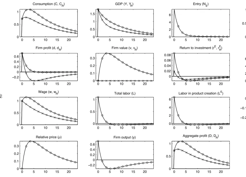
Figure 1 shows the responses of key endogenous variables to a 1 percent positive innovation to Zt under C.E.S. preferences. The number of years after the shock is on the horizontal axis. The
responses for all real variables are shown using both the welfare-relevant price index Pt(represented
as dots) and the data-consistent CPI price index pt (represented as crosses). Both measures are
important. The data-consistent series provides the link back to the empirical evidence. On the other hand, the dynamics are driven by optimizing behavior with respect to their welfare-relevant counterparts.
1 5The period utility function is de…ned over leisure (1 L
t) in King and Rebelo (1999), where the endowment of
time in each period is normalized to 1. The elasticity of labor supply is then the risk aversion to variations in leisure (set to 1 in their benchmark calibration) multiplied by (1 L)=L, where L is steady-state e¤ort, calibrated to 1=5. This yields ' = 4 in our speci…cation.
Consider …rst the e¤ects of the shock on impact. Note that the relative price t pt=Ptdepends
only on the number of products Nt, and is thus pre-determined at time t. The impact responses for
both the data- and welfare-consistent measures are thus identical. The productivity improvement spurs pro…t expectations generated by the increased demand for all individual goods yt. Absent any
entry, this would translate into a higher (ex-ante) value for each variety. However, the free entry mechanism induces an immediate response of entry that drives the (ex-post) equilibrium value of a variety back down to the level of the entry cost; recall that this is equal to the marginal cost of producing an extra unit of an existing good. Since marginal cost (and hence the entry cost) moves in lockstep with the -constant on impact- individual relative price ( t), it follows that on impact
there is no reaction in marginal cost; Therefore, entry occurs up to the point where the (ex-post) equilibrium …rm value does not react to the shock on impact.
The remaining question is then what is the optimal relative allocation of the productivity increase between the two sectors: consumption Ct and investment (entry) NE;t. To understand
why consumption increases less than proportionally with productivity it is important to consider the investment decision of households. The price of a share (value of a …rm) together with its payo¤ (dividends obtained from monopolistic …rms) determine the return on a share: the return to entry (product creation). On impact, the rate of return to investing (rE
t+1, evaluated from the
ex ante perspective of investment decisions) is high, both because the present share price is low relative to the future and because next period’s share payo¤s (…rm pro…ts) are expected to be high. Intertemporal substitution logic implies that the household should postpone consumption into the future; Since the only means to transfer resources intertemporally is the introduction of new varieties, investment (measured either as the number of entrants NE;t or in consumption units
ItE vtNE;t) increases on impact; This is the mirror (“demand”) image of the new …rms’ decision
to enter discussed earlier. This allocation of resources, driven by intertemporal substitution, is also re‡ected in the allocation of labor across the two sectors: On impact, labor is reallocated into product creation (LE
t) from the production of existing goods (LCt).17 Lastly, the real wage increases
on impact in line with the increase in productivity; and faced with this higher wage, the household
1 7The negative correlation between labor inputs in the two sectors of our economy is inconsistent with evidence
concerning sectoral comovement. This feature, however, is shared by all multi-sector models in which labor is perfectly mobile (see Christiano and Fitzgerald, 1998, for an early review of the evidence and implications for a two-sector RBC model). One natural way to induce comovement would be to introduce costs of reallocating labor across sectors as in Boldrin, Christiano, and Fisher (2001).
optimally decides to work more hours in order to attain a higher consumption level. GDP (Yt)
increases because both consumption and investment increase.
Over time, increased entry translates into a gradual increase in the number of products Nt
and reduces individual good demand (output of each good falls below the steady state for most of the transition). More product variety also generates a love-of-variety welfare e¤ect that is re‡ected in the increase in the relative price t. This increase is also re‡ected one-for-one in the
welfare-consistent measure of the value of a variety (since the opportunity cost of investment in terms of foregone consumption is now higher with more varieties). Pro…ts per variety fall with the reduction in demand per variety. Together with the higher opportunity cost of investment from higher product variety, this generates a fall in the return to investment/entry below its steady state value and a reversal in the allocation of labor: labor is reallocated back from product creation to production. The hump-shaped pattern of aggregate consumption is consistent with the dynamics of the return to investment. After a certain amount of time, the number of products peaks, and then progressively declines back to its old steady state level. This also unwinds the welfare e¤ects driven by the additional product variety ( t decreases). The decrease in product variety is also
re‡ected in a reversal of the decrease in individual good demand and pro…ts per-variety, which then increase back up to their steady state levels. Importantly, however, aggregate pro…t Dt Ntdtand
its data consistent counterpart DR;t remain above the steady state throughout the transition. The
response of data-consistent consumption (CR;t) is still hump-shaped, but relatively more muted
than its welfare consistent counterpart as it does not factor in the additional bene…ts from product variety. The data-consistent …rm value is constant because with C.E.S. preferences the markup is constant, namely vR;t= fE= = fE( 1) = . Finally, the data-consistent real wage wR;t declines
monotonically toward the steady state, tracking the behavior of productivity.18
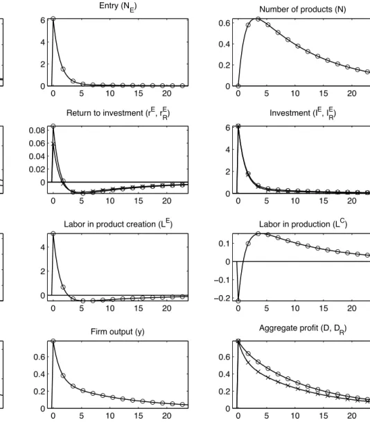
Figure 2 repeats the experiment of Figure 1 for the case of translog preferences. The qualitative behavior of several variables is similar to the C.E.S. case, but key di¤erences emerge. With translog preferences, varieties become closer substitutes as the increased product variety induces a crowding-out e¤ect in product space. These demand side changes, in turn, lead to lower markups. Relative to
1 8The welfare-consistent real wage w
t increase by more than productivity in all periods after impact, because a
higher number of …rms puts upward pressure on labor demand. With logarithmic utility from consumption, labor supply depends on wt=Ct = wR;t=CR;t. In other words, variety has no e¤ect on labor supply. This would no longer
C.E.S., the pro…t incentive for product creation is thus weaker, and is re‡ected in a muted response of entry. However, the hump-shape response for overall product variety is still very similar to the C.E.S. case, and this induces the countercyclical response of the markup, t, which declines over
time before settling on the path back to the steady state.19 The muted response of the relative price under translog preferences implies that individual …rm output does not drop below the steady state during the transition (as it did in the C.E.S. case): it is relatively more pro…table to keep producing old goods, since investing in new ones erodes pro…t margins and yields a smaller welfare gain to consumers. This is also evident in the dynamics of labor across sectors: the reallocation of labor from product creation back into the production of existing goods takes place faster than in the C.E.S. case.
Importantly, although markups are countercyclical, aggregate pro…ts (both welfare- and data-consistent) remain strongly pro-cyclical. It is notoriously di¢cult to generate both countercyclical markups and procyclical aggregate pro…ts in models with a constant number of producers/products (for instance, based on sticky prices). These models imply that pro…ts become countercyclical, in stark contrast with the data (see Rotemberg and Woodford, 1999). Our model naturally breaks this link between the responses of markups and aggregate pro…ts via the endogenous ‡uctuation in the number of products. Procyclical product entry pushes up aggregate pro…ts relative to the change in the product-level markup. We return to this issue when computing the second moments of our arti…cial economy below.20
Finally, we note that these responses di¤er from the e¢cient ones generated by solving the social planner’s problem for our economy. There is the standard markup distortion of the di¤erentiated goods relative to leisure (this is also a feature of models without endogenous entry). Moreover, an intertemporal distortion occurs when the markups on goods are not synchronized over time. Lastly, endogenous entry generates another distortion whenever the incentives for entry are not aligned with the welfare bene…t of product variety. The C.E.S. preferences introduced by Dixit and Stiglitz
1 9The ‡uctuations of the markup over time, also generate di¤erences relative to the C.E.S. responses for
data-consistent measures. For example, the data data-consistent value of a variety vR;t= fE= (Nt) increases with the markup,
since the latter implies a higher opportunity cost of foregone production.
2 0A discussion of the responses to a permanent increase in productivity can be found in Bilbiie, Ghironi, and Melitz
(2007), along with a discussion of the consequences of di¤erent values for the elasticity of labor supply. The most salient feature of the responses to a permanent shock is that, with C.E.S. preferences, GDP expansion takes place entirely at the intensive margin in the short run, while it is entirely driven by the extensive margin (with …rm-level output back at the initial steady state) in the long run. With translog preferences, extensive and intensive margin adjustments coexist in the long run.
(1977) represent a knife-edge case that eliminates those last two distortions. On the other hand, the translog case compounds all three distortions. See Bilbiie, Ghironi, and Melitz (2008a) for a detailed discussion of these distortions and the associated planner remedies.
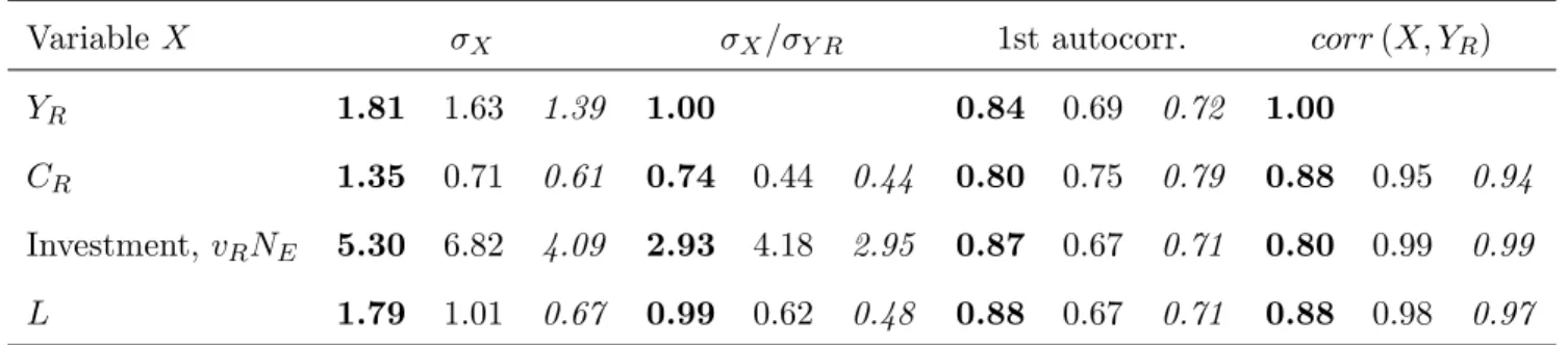
3.3 Second Moments
To further evaluate the properties of our baseline model, we compute the implied second moments of our arti…cial economy for some key macroeconomic variables and compare them to those of the data and those produced by the benchmark RBC model. While discussing the behavior of welfare-consistent variables was important to understand the impulse responses above, here we focus only on empirically relevant variables, as we compare the implications of the model to the data. Table 3 presents the results for our C.E.S. model.21 In each column, the …rst number (bold fonts) is the empirical moment implied by the U.S. data reported in King and Rebelo (1999), the second number (normal fonts) is the moment implied by our model, and the third number (italics) is the moment generated by King and Rebelo’s baseline RBC model. We compute model-implied second moments for HP-…ltered variables for consistency with data and standard RBC practice, and we measure investment in our model with the real value of household investment in new …rms (vRNE).
Remarkably, the performance of the simplest model with entry subject to sunk costs and con-stant markups is similar to that of the baseline RBC model in reproducing some key features of U.S. business cycles. Our model fares better insofar as reproducing the volatilities of output and hours. The ratio between model and data standard deviations of output is 0:90, compared to 0:77 for the standard RBC model; and the standard deviation of hours is 50 percent larger than that implied by the RBC model. On the other hand, investment is too volatile, and our baseline framework faces the same well-known di¢culties of the standard RBC model: Consumption is too smooth relative to output; there is not enough endogenous persistence (as indicated by the …rst-order autocorrelations); and all variables are too procyclical relative to the data.
Additionally, however, our model can jointly reproduce important facts about product creation and the dynamics of pro…ts and markups: procyclical entry (as reviewed in the Introduction), procyclical pro…ts, and, in the version with translog preferences, countercyclical markups. To
2 1The moments in Table 3 change only slightly under translog preferences, without a¤ecting the main conclusions.
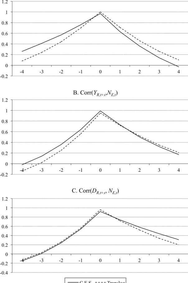
substantiate this point, Figure 3 plots model-generated cross-correlations of entry, aggregate real pro…ts, and GDP for C.E.S preferences and translog preferences. In both cases, entry and pro…ts are strongly procyclical, and the contemporaneous correlation of pro…ts and entry is positive.22 Figure 4 shows the model-generated correlation of the markup with GDP at various lags and leads under translog preferences, comparing it to that documented by Rotemberg and Woodford (1999). Our model almost perfectly reproduces the contemporaneous countercyclicality of the markup; furthermore, the time pro…le of its correlation with the business cycle also matches well with the empirical evidence.23 There is a straightforward intuition for this result, which follows from the
slow movement of the number of …rms in our model: When productivity increases, GDP increases on impact and then declines toward the steady state, while the number of …rms builds up gradually before returning to the steady state. Since the markup is a decreasing function of the number of …rms, it also falls gradually in response to a technology shocks. As a consequence, the markup is more negatively correlated with lags of GDP and positively correlated with its leads.
We view the performance of our model as a relative success. First, the model, although based on a di¤erent propagation mechanism from which traditional physical capital is absent, has second moment properties that are comparable to the RBC model concerning macroeconomic variables of which that model speaks; indeed, our model fares better insofar as generating output and hours volatility is concerned. Second, our model can explain (at least qualitatively) stylized facts about which the benchmark RBC model is silent. Third, to the best our knowledge, our model is the …rst that can account for all these additional facts simultaneously: Earlier models that address entry (such as those we discuss in Section 5) fail to account for the cyclicality of pro…ts (since they assume entry subject to a period-by-period zero pro…t condition), and models that generate procyclical pro…ts (due to monopolistic competition) abstract from changes in product space. Finally, we view the ability to generate procyclical pro…ts with a countercyclical markup and to reproduce the time
2 2In Bilbiie, Ghironi, and Melitz (2007), we show that the tent-shaped patterns in Figure 3 are not too distant from
reproducing the evidence for net …rm entry as measured by the di¤erence between new incorporations and failures.
2 3Of the various labor share-based empirical measures of the markup considered by Rotemberg and Woodford, the
one that is most closely related to the markup in our model is the version with overhead labor, whose cyclicality is reported in column 2 of their Table 2, page 1066, and reproduced in Figure 4. In our model, the inverse of the markup is equal to the share of production labor (labor net of workers in the “investment” sector who develop new products) in total consumption: 1= t = [wt(Lt LE;t)] =Ct. This also implies that the share of aggregate pro…ts
in consumption is the remaining share 1 (1= t). Countercyclical markups therefore entail a countercyclical pro…t
share and a procyclical labor share, as documented by Rotemberg and Woodford (1999). Those authors also measure shares in consumption rather than GDP. Since the share of consumption in GDP is relatively acyclical, this di¤erence in the use of denominators will not be consequential.
pattern of the markup’s correlation with the cycle in the simplest version of our model as major improvements relative to other (e.g., sticky-price-based) theories of cyclical markup variation.
4 The Role of Physical Capital
We now extend our model and incorporate physical capital as well as the capital embodied in the stock of available product lines. We explore this for two reasons. First, our benchmark model studies an extreme case in which all investment goes toward the creation of new production lines and their associated products. While this is useful to emphasize the new transmission mechanism provided by producer entry, it is certainly unrealistic: Part of observed investment is accounted for by the need to augment the capital stock used in production of existing goods. Second, the introduction of physical capital may improve the model’s performance in explaining observed macroeconomic ‡uctuations. Since inclusion of capital in the model does not represent a major modeling innovation, we relegate the presentation of the augmented setup to the Appendix, and limit ourselves to mentioning the main assumptions here.
We assume that households accumulate the stock of capital (Kt), and rent it to …rms producing
at time t in a competitive capital market. Investment in the physical capital stock (It) requires
the use of the same composite of all available varieties as the consumption basket. Physical capital obeys a standard law of motion with rate of depreciation K 2 (0; 1). For simplicity, we follow Grossman and Helpman (1991) and assume that the creation of new …rms does not require physical capital. Producing …rms then use capital and labor to produce goods according to the Cobb-Douglas production function yt(!) = Ztlt(!) kt(!)1 ,with 0 < < 1.
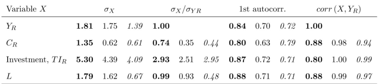
As with the baseline model, we use the model with physical capital to compute second moments of the simulated economy. Table 4 reports results for key macro aggregates, for C.E.S. preferences (normal fonts) compared again to data and moments of the baseline RBC model (bold and italic fonts respectively).24 All parameters take the same values as in Section 3; in addition, the labor
share parameter is set to = 0:67 and physical capital depreciation to K = 0:025; values that
are standard in the RBC literature (e.g. King and Rebelo, 1999). For comparison with investment
2 4To save space, we do not report impulse responses for the model with capital. These, as well as second moments
for the translog case (which are not signi…cantly di¤erent from those in Table 4 for the relevant variables) are available upon request.
data, we now measure investment with the real value of total investment in physical capital and new …rm creation, T IR;t vR;tNE;t+IR;t, where IR;tis real investment in physical capital accumulation.
Inclusion of physical capital alters some of the key second-moment properties of the model rel-ative to Table 3. In particular, the model with capital reproduces almost the entire data variability of output and hours worked, thus clearly outperforming both our baseline and the RBC model (the ratio between model and data standard deviations of output is 0:97, while the relative standard deviation of hours is twice as large as that implied by the RBC model). The volatility of invest-ment is also much closer to its data counterpart (whereas in our baseline model without physical capital investment was too volatile). On a more negative note, the model still generates too smooth consumption, fails to reproduce persistence, and overstates correlations; all these shortcomings are shared with the baseline RBC model and many of its extensions. Lastly, the correlations pertain-ing to entry, pro…ts, and markup are not signi…cantly a¤ected with respect to the baseline model without physical capital (results available upon request). In summary, we show that the incorpo-ration of physical capital signi…cantly a¤ects some of the business cycle properties of the model, in particular those pertaining to volatility of output, hours, and investment, bringing them closer to the data.
5 Discussion: Entry in Business Cycle Models
We argued that the introduction of endogenous producer entry and product variety is a promising avenue for business cycle research, for the ability of the mechanism to explain several features of evidence and improve upon the basic RBC setup. To be fair, ours is not the …rst paper that introduces producer entry in a business cycle framework. But our model di¤ers from earlier ones along important dimensions. In this section, we discuss the relation between our model and earlier models with producer entry, as well as some recent studies in the same vein.
Chatterjee and Cooper (1993) and Devereux, Head, and Lapham (1996a,b) documented the procyclical nature of entry and developed general equilibrium models with monopolistic competition to study the e¤ect of entry and exit on the dynamics of the business cycle. However, entry is frictionless in their models: There is no sunk entry cost, and …rms enter instantaneously in each period until all pro…t opportunities are exploited. A …xed period-by-period cost then serves to
bound the number of operating …rms. Free-entry implies zero pro…ts in all periods, and the number of producing …rms in each period is not a state variable. Thus, these models cannot jointly address the procyclicality of pro…ts and entry. In contrast, entry in our model is subject to a sunk entry cost and a time-to-build lag, and the free entry condition equates the expected present discounted value of pro…ts to the sunk cost.25 Thus, pro…ts are allowed to vary and the number of …rms is a state variable in our model, consistent with evidence and the widespread view that the number of producing …rms is …xed in the short run.26 Finally, our model exhibits a steady state in which: (i)
The share of pro…ts in capital is constant and (ii) the share of investment is positively correlated with the share of pro…ts. These are among the Kaldorian growth facts outlined in Cooley and Prescott (1995), which neither the standard RBC model nor the frictionless entry model can account for (the former because it is based on perfect competition, the latter because the share of pro…ts is zero).
Entry subject to sunk costs, with the implications that we stressed above, also distinguishes our model from more recent contributions such as Comin and Gertler (2006) and Jaimovich and Floetotto (2008), who also assume a period-by-period, zero-pro…t condition.27 Our model further di¤ers from Comin and Gertler’s along three dimensions: (i) We focus on a standard de…nition of the business cycle, whereas they focus on the innovative notion of “medium term” cycles; (ii) Our model generates countercyclical markups due to demand-side pricing complementarities, whereas Comin and Gertler, like Galí (1995), postulate a function for markups which is decreasing in the number of …rms; (iii) Our model features exogenous, RBC-type productivity shocks, whereas Comin and Gertler consider endogenous technology and use wage markup shocks as the source
2 5The pattern of product creation and destruction documented by Bernard, Redding, and Schott (2010) and Broda
and Weinstein (2010) is also most consistent with sunk product development costs subject to uncertainty – as featured in our model.
2 6In fact, our model features a …xed number of producing …rms within each period and a fully ‡exible number
of …rms in the long run. Ambler and Cardia (1998) and Cook (2001) take a …rst step in our direction. A period-by-period zero pro…t condition holds only in expectation in their models, allowing for ex post pro…t variation in response to unexpected shocks, and the number of …rms in each period is predetermined relative to shocks in that period. Benassy (1996) analyzes the persistence properties of a variant of the model developed by Devereux, Head, and Lapham (1996a,b).
2 7Sunk entry costs are a feature of Hopenhayn and Rogerson’s (1993) model, which is designed to analyze the
employment consequences of …rm entry and exit, and thus directly addresses the evidence in Davis, Haltiwanger, and Schuh (1996). However, Hopenhayn and Rogerson assume perfect competition in goods markets (as in Hopenhayn’s, 1992, seminal model) and abstract from aggregate dynamics by focusing on stationary equilibria in which prices, employment, output, and the number of …rms are all constant. Lewis (2006) builds on the framework of this paper and estimates VAR responses (including those of pro…ts and entry as measured by net business formation) to macroeconomic shocks, …nding support for the sunk-cost driven dynamics predicted by our model.