Constraining global methane emissions and uptake by ecosystems

HAL Id: hal-03203163

https://hal.archives-ouvertes.fr/hal-03203163

Submitted on 21 Apr 2021

HAL is a multi-disciplinary open access

archive for the deposit and dissemination of

sci-entific research documents, whether they are

pub-lished or not. The documents may come from

teaching and research institutions in France or

abroad, or from public or private research centers.

L’archive ouverte pluridisciplinaire HAL, est

destinée au dépôt et à la diffusion de documents

scientifiques de niveau recherche, publiés ou non,

émanant des établissements d’enseignement et de

recherche français ou étrangers, des laboratoires

publics ou privés.

ecosystems

R. Spahni, R. Wania, L. Neef, M. van Weele, I. Pison, P. Bousquet, C.

Frankenberg, P. Foster, F. Joos, I. Prentice, et al.

To cite this version:

R. Spahni, R. Wania, L. Neef, M. van Weele, I. Pison, et al.. Constraining global methane emissions

and uptake by ecosystems. Biogeosciences, European Geosciences Union, 2011, 8 (6), pp.1643-1665.

�10.5194/bg-8-1643-2011�. �hal-03203163�

www.biogeosciences.net/8/1643/2011/ doi:10.5194/bg-8-1643-2011

© Author(s) 2011. CC Attribution 3.0 License.

Biogeosciences

Constraining global methane emissions and uptake by ecosystems

1_{Climate and Environmental Physics, Physics Institute, and Oeschger Centre for Climate Change Research,}

University of Bern, Bern, Switzerland

2_{QUEST, Department of Earth Sciences, University of Bristol, Bristol, UK}

3_{School of Earth and Ocean Sciences, University of Victoria, Victoria, British Columbia, Canada}

4_{KNMI, Royal Netherlands Meteorological Institute, De Bilt, The Netherlands}

5_{Earth System modeling, Helmholtz Centre Potsdam, Potsdam, Germany}

6_{Laboratoire des Sciences du Climat et de l’Environnement (LSCE), Gif-sur-Yvette, France}

7_{Netherlands Institute for Space Research, Utrecht, The Netherlands}

8_{Department of Biological Sciences, Macquarie University, North Ryde, NSW 2109, Australia}

9_{Grantham Institute and Division of Biology, Imperial College, Ascot SL5 7PY, UK}

*_{now at: Jet Propulsion Laboratory, California Institute of Technology, Pasadena, USA}

Received: 28 October 2010 – Published in Biogeosciences Discuss.: 11 January 2011 Revised: 20 May 2011 – Accepted: 30 May 2011 – Published: 23 June 2011

Abstract. Natural methane (CH4) emissions from wet

ecosystems are an important part of today’s global CH4

bud-get. Climate affects the exchange of CH4between

ecosys-tems and the atmosphere by influencing CH4production,

ox-idation, and transport in the soil. The net CH4exchange de-pends on ecosystem hydrology, soil and vegetation charac-teristics. Here, the LPJ-WHyMe global dynamical

vegeta-tion model is used to simulate global net CH4emissions for

different ecosystems: northern peatlands (45◦–90◦N), natu-rally inundated wetlands (60◦S–45◦N), rice agriculture and wet mineral soils. Mineral soils are a potential CH4sink, but can also be a source with the direction of the net exchange de-pending on soil moisture content. The geographical and sea-sonal distributions are evaluated against multi-dimensional atmospheric inversions for 2003–2005, using two indepen-dent four-dimensional variational assimilation systems. The atmospheric inversions are constrained by the atmospheric

CH4 observations of the SCIAMACHY satellite instrument

and global surface networks. Compared to LPJ-WHyMe the inversions result in a significant reduction in the emissions from northern peatlands and suggest that LPJ-WHyMe max-imum annual emissions peak about one month late. The

Correspondence to: R. Spahni

([email protected])

inversions do not put strong constraints on the division of sources between inundated wetlands and wet mineral soils in the tropics. Based on the inversion results we diagnose model parameters in LPJ-WHyMe and simulate the surface

exchange of CH4over the period 1990–2008. Over the whole

period we infer an increase of global ecosystem CH4

emis-sions of +1.11 Tg CH4yr−1, not considering potential addi-tional changes in wetland extent. The increase in simulated CH4emissions is attributed to enhanced soil respiration re-sulting from the observed rise in land temperature and in at-mospheric carbon dioxide that were used as input. The

long-term decline of the atmospheric CH4growth rate from 1990

to 2006 cannot be fully explained with the simulated ecosys-tem emissions. However, these emissions show an

increas-ing trend of +3.62 Tg CH4yr−1over 2005–2008 which can

partly explain the renewed increase in atmospheric CH4

con-centration during recent years.

1 Introduction

1.1 General introduction

Anthropogenic methane (CH4) emissions contribute

signifi-cantly to global radiative forcing. Since pre-industrial times

a current forcing of 0.48 W m−2 _{(Denman et al., 2007).} This corresponds to ∼ 30 % of the radiative forcing from

CO2 (1.66 W m−2). In addition, present-day global

nat-ural CH4 emissions are estimated to be 145–260 Tg yr−1

(1 Tg yr−1=1012g CH4yr−1), which is ∼25–50 % of total

CH4emissions (∼503–610 Tg yr−1) (Denman et al., 2007).

The goal of this study is to identify trends and variability

of global net CH4 exchange from ecosystems over the last

two decades. We also make a first attempt to attribute the variability of CH4exchange to different categories of ecosys-tems on the global scale. In the existing literature,

biogeo-chemical processes leading to CH4exchanges are commonly

treated identically as emissions from “wetlands”. Here we try to assess these processes individually by modelling the biogeochemical cycle of the land biosphere, the atmospheric

chemistry and transport of emitted CH4, and the

uncertain-ties associated with these processes.

1.2 Uncertainties and variability

The uncertainty in total natural CH4 emissions is mainly

due to lack of knowledge of the geographical distribution

and interannual variability of CH4 emissions from

ecosys-tems, the largest natural source (Denman et al., 2007).

In-verse (“top-down”) modelling of atmospheric CH4emissions

suggests that interannual variability of wet ecosystem emis-sions is ± 12 Tg yr−1, which explains about 70 % of global emission anomalies over the period 1984–2003 (Bousquet

et al., 2006). Interannual variability in CH4 loss

addition-ally contributes to the uncertainty of the global CH4budget

and thereby the inferred emissions. In the free troposphere

CH4 molecules are photochemically destroyed by reaction

with hydroxyl radicals (OH). The tropospheric OH loss rep-resents the main global CH4sink (∼428–511 Tg yr−1) (Den-man et al., 2007). The largest loss and, thus, the shortest CH4life time is found in the tropical troposphere, where the

primary production of OH radicals from ozone (O3)

photol-ysis is most efficient because of the combination of strong ultraviolet radiation intensity and high humidity. Taking into

account a stratospheric sink of ∼40 Tg yr−1 and CH4

con-sumption in soils of ∼30 Tg yr−1, the present-day global

chemical CH4life time is estimated to be within the range

8.45 ± 0.38 yr (Stevenson et al., 2006). The debate on the interannual variability in OH-loss in recent decades (Forster et al., 2007; Prinn et al., 2005; Montzka et al., 2011) is still unresolved.

Atmospheric CH4 concentration remained roughly stable

during the late 1990s to 2006. This points to a

tempo-rary balance between sources and sinks. Atmospheric CH4

concentrations started to rise again from the year 2007 on-ward (Rigby et al., 2008; Dlugokencky et al., 2009). The renewed increase seems to reflect growing anthropogenic

emissions of CH4 (EC-JRC/PBL, 2009), while the

tempo-rary balance does not. The rapid rise in anthropogenic

pol-lution of atmospheric constituents like NOx, predominantly

at (sub-)tropical latitudes, may lead to enhanced ozone for-mation and therefore higher OH concentrations that reduce

the chemical lifetime of tropospheric CH4(Dalsøren et al.,

2009; van Weele and van Velthoven, 2010).

The period of stabilisation has been explained by decreas-ing anthropogenic emissions until 1999, followed by a de-cline in wetland emissions (Bousquet et al., 2006). How-ever, the ecological, biogeochemical, thermal and

hydrolog-ical processes governing CH4exchange between ecosystems

and the atmosphere are poorly constrained on the global scale. Thus, estimates of global emissions are often calcu-lated using simple parametrisations (e.g., Kaplan, 2002), but process based “bottom-up” emission models have become available in the last decade (e.g., Walter et al., 2001a,b; Ket-tunen, 2003; Zhuang et al., 2004; Wania et al., 2010a).

1.3 Approach description

Here we use the Lund-Potsdam-Jena dynamic global vegeta-tion model (DGVM) with Wetland Hydrology and Methane (LPJ-WHyMe), that includes permafrost dynamics, peatland hydrology and peatland vegetation (Wania et al., 2009a,b),

to simulate CH4 emissions from northern peatlands

(Wa-nia et al., 2010a). Global model output of LPJ-WHyMe is used to parametrise emissions from inundated wetlands

south of 45◦N, rice agriculture and wet mineral soils, and

to parametrise CH4uptake by soils.

We combine this “bottom-up” model approach with two “top-down” atmospheric inversions using the LMDz-SACS (Pison et al., 2009) and TM5-4Dvar (Bergamaschi et al., 2007; Meirink et al., 2008a,b) assimilation frameworks for

the years 2003–2005. The inversions are constrained by CH4

concentration observations from the SCIAMACHY satellite instrument (Frankenberg et al., 2008) and by the observations

of the global CH4ground-based networks

(GLOBALVIEW-CH4, 2009).

In an iterative approach, we separate and test emission dis-tributions that are based on detailed process modelling and parametrisations on a global scale. Net exchange fluxes from

LPJ-WHyMe are constrained by their spatial (1◦by 1◦grid)

and temporal (monthly) patterns, and their agreement with chemistry, transport and concentrations in the atmosphere. In Sect. 2 we describe the models used for the biogeochemical and the atmospheric inverse modelling. The separation into different source and sink categories based on the involved process schemes is explained in Sect. 3. Emission distribu-tions and climate-induced trends and budgets for the period 1990–2008 are presented in Sect. 4. Finally, the results are discussed (Sect. 5) and summarised (Sect. 6).

2 Modelling framework

2.1 Biogeochemical process modelling

For the “bottom-up” biogeochemical process modelling of

CH4emissions we apply LPJ-WHyMe v1.3 (hereafter LPJ)

for (i) high-northern-latitude peatlands (45◦–90◦N) and for (ii) global mineral soils.

(i) In high-northern-latitude peatlands (hereafter northern peatlands), LPJ simulates peatland vegetation (either the peatland specific plant functional types (PFTs) of flood tolerant C3 graminoids, and, Sphagnum mosses or any of the generic PFTs depending on the inunda-tion status), soil temperature (freezing and thawing), permafrost dynamics (active layer depth), peatland hy-drology (evapotranspiration, water table position) and snow cover (Wania et al., 2009a). Additionally, LPJ simulates the carbon balance of the peat, thus the soil carbon stock, carbon accumulation and decomposition rates (Wania et al., 2009b). The soil carbon serves as a substrate for methanogenesis parametrised as a frac-tion of soil heterotrophic respirafrac-tion (HR). CH4is trans-ported to the surface by plant mediated transport, by dif-fusion through the soil or by ebullition. CH4is oxidised under aerobic conditions in the soil layer and during transport (Wania et al., 2010b).

(ii) On mineral soils, LPJ simulates natural vegetation dy-namics of 10 PFTs, soil hydrology (evapotranspiration, soil moisture), soil temperatures (freezing and thaw-ing) and snow cover (Sitch et al., 2003; Gerten et al., 2004; Wania et al., 2009a) using non-peatland hydrol-ogy in the model. The use of peatland and non-peatland hydrology depends on the soil class, but can also be switched off completely. LPJ gives estimates for the land carbon pools and soil HR rates depending on tem-perature and soil moisture content (Wania et al., 2009b). Versions of LPJ have been applied to study the global carbon cycle in the past (e.g., Joos et al., 2004) and the

future (e.g., Sitch et al., 2008). CH4 soil fluxes from

mineral soils are estimated by using relationships

be-tween CH4 emissions and soil HR, soil moisture and

temperature simulated by LPJ as described in the next section.

The Climate Research Unit (CRU) TS 3.0 climate data set (Mitchell and Jones, 2005) is used to force LPJ. Monthly in-put data to LPJ are surface air temperature, total precipita-tion, fractional sunshine hours from cloud cover percentage, and number of wet days from the CRU climatology. Addi-tionally, the CRUNCEP data set was used to perform sim-ulations for the period 1990–2008 (Viovy and Ciais, 2009, personal communication). The model spin-up procedure and other input data are described in Wania et al. (2009a, 2010a).

2.2 Inverse atmospheric modelling using four-dimensional data assimilation

Inversions of trace gas emissions constrained by surface as well as satellite-borne observations are a powerful tool for the validation of emission distributions and their trends and variability. Inversions based in 4D variational data assimila-tion (4D-Var, Houweling et al., 1999; Meirink et al., 2008a,b; Pison et al., 2009), which use the adjoint of a chemistry transport model to correct fluxes such that the fit between observed and modelled concentration is improved, are espe-cially powerful.

Here we use two 4D-Var inversion systems: TM5-4Dvar (Bergamaschi et al., 2007, 2009; Meirink et al., 2008a,b) and LMDz-SACS (Pison et al., 2009). For the tracer-transport

model TM5, the 4D-Var inversion framework optimises CH4

flux per model-grid-box per emission category per month. Therefore, it is used to test in a diagnostic way the

biogeo-chemically modelled CH4 emissions per category by LPJ.

This inversion system has no interactive chemistry, with CH4 loss parametrised with a prescribed OH field (Bergamaschi et al., 2007). In contrast the LMDz-SACS inversion frame-work simultaneously inverts three chemical species (methane

– CH4, carbon monoxid – CO, hydrogen – H2) and has

in-teractive chemistry (Pison et al., 2009). While TM5-4Dvar solves for fluxes per category, LMDz-SACS solves for total

monthly CH4flux per model grid-box. The full description

of both inversion systems is given in Appendix B.

3 Methane source and sink categories

Among the natural sources of CH4we focus on biogenic soil

emissions and subdivide them by type of ecosystem. Many different global classifications categorise potentially CH4 -producing ecosystems by hydrology, geomorphology, salin-ity, soil composition, vegetation, biogeochemistry, or a com-bination of these (e.g., Matthews and Fung, 1987; Semeniuk and Semeniuk, 1997). Here we use a classification with re-spect to the processes relevant for the microbial production,

oxidation and transport of CH4 in natural soils. The

clas-sification is simplified to three types: peatlands, inundated wetlands (including rice agriculture), and mineral soils. In

addition, we simulate CH4uptake in mineral soils and

pre-scribe anthropogenic emissions from the EDGAR inventory

(EC-JRC/PBL, 2009) as well as some smaller natural CH4

sources (Sect. 3.4). In the following Sects. 3.1–3.3 we ex-plain the calculation and parametrisation of sources and sinks in more detail. We test two emission scenarios, SC1 and SC2 (summarised in Table 1 and discussed in Sect. 4) for their

consistency with the observed CH4concentrations.

3.1 Northern peatlands

Peatlands are important ecosystems in northern high

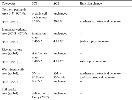
Table 1. Differences in model setup and modelled CH₄surface fluxes (global 1◦×1◦grid) between LPJ scenarios SC1 and SC2. Emission changes were achieved by changing source area or source strength in SC2 (column 3 and 4). The area assigned to the category wet mineral soils and their CH4emissions were considerably reduced in SC2 by raising the threshold of soil moisture (SM), expressed as fraction of the

water holding capacity (whc), above which CH4emissions can occur.

Categories SC1 SC2 Emission change Northern peatlands

Area (45◦–90◦N): organic soil unchanged – carbon map

rC[CH4]/C[CO2]: 25.0 % 20.0 % northern extra-tropical decrease Inundated wetlands

area (60◦S– 45◦N): inundation unchanged – map

rC[CH4]/C[CO2]: 2.40 %

∗ _{4.15 %}∗ _{(sub-)tropical increase}

Rice agriculture

area (global): rice fraction unchanged – map

rC[CH4]/C[CO2]: 2.40 %

∗

4.15 %∗ sub-tropical increase

Wet mineral soils

area (global): SM > SM > northern extra-tropical decrease 85 % whc 95 % whc and small tropical decrease

rC[CH4]/C[CO2]: 0.52 %

∗ _{unchanged –}

Soil uptake

area (global): defined as in Curry (2007)

unchanged –

∗_{Here, the carbon conversion factor also includes oxidation of CH}

4to CO2during transport to the surface and general flux tuning.

organic matter. Peat layer growth and decomposition de-pend principally on its composition and the water table po-sition, and to a lesser extent also on soil temperature (Rouse et al., 1997). Peatland formation in the arctic, boreal and alpine regions is spatially and temporally influenced by the occurrence of permafrost (Robinson and Moore, 2000). LPJ directly simulates these physical processes and in addition,

CH4 production, oxidation and transport to the atmosphere

(Wania et al., 2010b). The production term is calculated pro-portional to HR in the soil, where HR depends on the mass (Mi) of each individual LPJ carbon pool (CP) in g C and the

associated turnover rate ki (yr−1):

HR =X i∈CP ki·Mi= X i∈CP k10_i ·RT·Rmoist·Mi (1)

Turnover rates (k_i10) at 10◦_{C for the exudates, aboveground}

and below-ground litter carbon pools, and fast and slow soil carbon pools are given in (Wania et al., 2010b). The

turnover rates increase with temperature (RT) (Lloyd and

Taylor, 1994) and have normalised exponential dependency with soil water content (Rmoist) (Fang and Moncrieff, 1999) for mineral soils. For peatlands Rmoist is set to a constant of

0.35 (Wania et al., 2010a). CH4 emissions are sensitive to

the carbon ratio of CH4to CO2production (rC[CH4]/C[CO2]),

which is applied to anoxic conditions but weighted by the volumetric fraction of air if a layer is not completely anoxic (Wania et al., 2010b). Due to some uncertainty of this value, we test two different values for rC[CH₄]/C[CO2]based on

com-parisons with site data, namely 25 % (SC1) and 20 % (SC2) (Wania et al., 2010a). The latter resulting in a lower methane production in peatlands. In our classification peatlands in-clude bogs, fens and mires, and are found predominantly in the Northern Hemisphere with an estimated maximum area

of 2.99–3.20×106km−2 (Matthews and Fung, 1987;

Asel-mann and Crutzen, 1989). As detailed in Sect. 6 of Wania et al. (2010a) and Sect. 3 of Wania et al. (2009a), we calcu-late the fractional peatland cover for the circumpolar region

(45◦–90◦N) from organic soil carbon content derived from

the IGBP-DIS 50×50resolution map (Global Soil Data Task

Group, 2000). The assumption in this approach is that high organic soil carbon content indicates areas where peat has been or currently is accumulating. After a comparison with the wetland area derived from a multiple satellite approach (Prigent et al., 2007) the peatland fractions derived from the IGBP-DIS data were further downscaled by a factor of 0.38 (Wania et al., 2010a). The resulting fractional peatland area

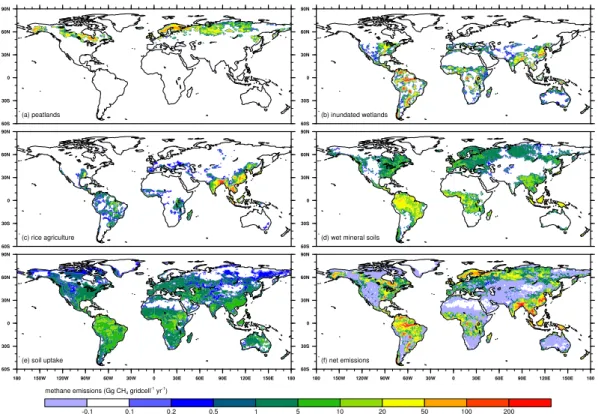
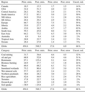
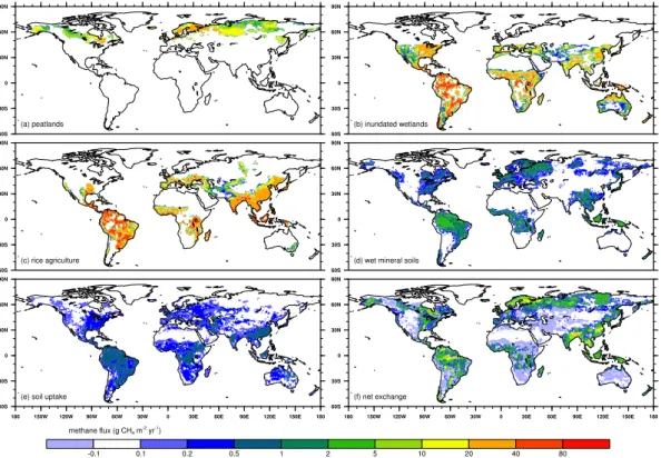
Fig. 1. CH4exchange by categories as simulated with LPJ for 2004 on a global grid (1◦×1◦) and with the settings of SC2: (a) Northern

extra-tropical peatlands based on a soil organic carbon map (Wania et al., 2010a), (b) inundated wetlands based on an inundation fraction map (Prigent et al., 2007), (c) rice agriculture based on a rice fraction map (Leff et al., 2004), (d) global wet mineral soils estimated using a threshold for soil moisture content in LPJ, (e) global soil uptake fluxes based on atmospheric surface concentrations (GLOBALVIEW-CH4,

2009) and the scheme by Curry (2007), and (f) net emissions from LPJ computed from the sum of all sources (a–d) minus soil uptake (e). Note the non-linear color scale in (a–f) and areas with negative numbers in (f), indicating an annual net CH4uptake.

(fpeat) between 45◦and 90◦N is about 2.05×106km−2. In addition, flux strengths are multiplied by a factor of 0.75 to take account of the micro-topographic heterogeneity found

in peatlands (Wania et al., 2010a). Total peatland

emis-sions for the circumpolar region are 51.1 Tg CH4(SC1) and

38.5 Tg CH4(SC2) for the year 2004 (Fig. 1a).

Tropical peatlands cover an area of ∼0.42×106km−2, pre-dominantly in South East (SE) Asia (Page et al., 2004). Thus, they represent ∼10–15 % of global peatland area. Tropical and boreal peatlands are, due to their climate regime, rather contrasting ecosystems in terms of hydrology, peat accumu-lation rate and inventory, and presumably sensitivities in CH4 emissions. Thus, we treat tropical peatlands separately from boreal peatlands: tropical peatlands are included in the class of inundated wetlands as described in the next section.

3.2 Naturally inundated wetlands and rice agriculture

Naturally inundated wetlands (60◦S to 45◦N) are

perma-nently flooded areas with a water table position close to the soil surface during the period of inundation. This category includes forest and non-forest swamps, marshes, peatlands and open water bodies in temporal, subtropical and tropical

regions. We use the inundation fraction data (0.25◦_×0.25◦

resolution) from a multi-satellite method (Prigent et al., 2007), and calculate the monthly mean fractional inunda-tion on the global 1◦×1◦ grid. A similar approach has re-cently been conducted for a global single wetland type source (Ringeval et al., 2010). The monthly fractional inundation data are available for the period 1993–2000. In this study we use the time-average mean fractional inundation for each month. In a sensitivity simulation, described in Sect. 4.3, the temporally varying data are prescribed for the period 1993– 2000 only.

Since satellite observations map all flooded areas, both naturally inundated and irrigated wetlands (i.e. fractional cover of rice agriculture) are included in the data set (Pri-gent et al., 2007). To separate naturally inundated wetlands from rice agriculture, we concatenate fractional inundation data with a map of fractional rice cover (Leff et al., 2004). Rice agricultural areas are concentrated in SE Asia and are an

important net source of atmospheric CH4of 31–112 Tg CH4

(Denman et al., 2007). However, more recent estimates

point to somewhat lower emissions of 14.8 to 41.7 Tg CH4

from rice agriculture (Yan et al., 2009). The fractional rice cover as given by Leff et al. (2004) is considered as an

annual maximum extent (fricemax). To get the monthly rice extent (frice), we truncate the fractional rice cover to the frac-tional inundation (finund) for each 1◦×1◦ grid cell (i) and each month (m). The remaining fractional area is then as-sumed to represent the fractional cover of naturally inundated wetlands (fnatwet):

frice,i,m=min(finund,i,m,fricemax,i,m) (2)

fnatwet,i,m=finund,i,m−frice,i,m (3)

With this separation it is possible to discriminate between

CH4 emissions from naturally inundated wetlands and

irri-gated rice agriculture. LPJ does not simulate CH4emissions

in a process-based way for temperate, sub-tropical and trop-ical ecosystems. Nevertheless, LPJ dynamtrop-ically simulates natural vegetation distribution (trees and grass), gross and net primary productivity, soil HR and related carbon pools (Sitch et al., 2003). Assuming that these natural soils develop anoxic conditions when being flooded, we expect that a frac-tion of carbon, respired in the soil, is released as CH4instead

of as CO2for the period of inundation. For CH4emissions

from naturally inundated wetlands and rice agriculture we directly modify the carbon conversion ratio rC[CH₄]/C[CO2]

to include CH4oxidation, transport and general flux tuning.

The modified ratio is thus lower than for peatland emissions, and set to 2.40 % (SC1) and 4.15 % (SC2) (see Appendix A) in agreement with previous estimates (Christensen et al., 1996). CH4emissions (einund) per m2and month (m) in grid cell i are then derived from soil HR as

einund,i,m=rC[CH4]/C[CO2]·HRi,m (4)

Enatwet,i,m=einund,i,m·fnatwet,i,m·Ai (5)

Erice,i,m=einund,i,m·frice,i,m·Ai (6)

where Enatwetand Ericeare total emissions from naturally in-undated wetlands and rice agriculture, respectively, per grid

cell with the area Ai (in m2). The global parametrisation

can be checked against regional emission inventories for rice agriculture in SE Asia (Fig. 2). The parametrised fluxes agree well with emission distributions and total estimates from the EDGAR data base (EC-JRC/PBL, 2009) with the exception that emissions in North-Western India along the Himalayan foothills are missing; this is due to a geographical mismatch of fractional rice cover (Leff et al., 2004) and precipitation input data, with low precipitation in the CRU input data

pre-venting vegetation growth and CH4production in LPJ in the

Indo-Gangetic Plain.

In summary, we simplify the classification of global wet ecosystems by latitude to prevent double counting of areas

and emissions. Wetlands north of 45◦N are considered to be

peatlands (fnatwet=0), whereas wetlands south of 45◦N are classified as inundated wetlands (fpeat=0). The reason for

the 45◦N cut-off line is that LPJ-WHyMe was specifically

Fig. 2. Methane emissions in Gg CH4from rice fields in SE Asia

for the year 2000. (a) Emissions are estimated from the

grid-ded distribution of fractional inundation (Prigent et al., 2007) and fractional rice cover (Leff et al., 2004) and assuming that 4.15 % of the heterotrophic respiration simulated by LPJ is converted to methane in inundated rice fields (scenario SC2). (b) Emissions from the EDGAR data (EC-JRC/PBL, 2009). Total emissions in SE Asia from rice cultivation are 36.4 and 36.6 Tg CH4from LPJ

and EDGAR, respectively. Resolution for both maps is 1◦×1◦.

developed for methane emissions from peatlands in cold ar-eas (either high latitude or high altitude), of which the

major-ity is found north of 45◦N. Since LPJ-WHyMe has not been

tested yet for wetlands other than this kind of peatland, we

chose to use the 45◦N cut-off as a boundary between

simu-lating CH4emissions within LPJ-WHyMe for northern

peat-lands and using a more generic correlation approach (Eqs. 4– 6) for the rest of the inundated areas. Additionally, seasonal rice agriculture is calculated from global fractional inunda-tion and global rice cover extent. The global distribuinunda-tion of these three sources are shown in Fig. 1a–c as fluxes per grid cell and additionally in Fig. A1a–c as fluxes per unit area.

Mineral soils that are not inundated can still be a net CH4 source. Soils with a low soil moisture content imply oxic

conditions which allow bacteria to consume CH4 (Curry,

2007, and refs. therein). Relatively high soil moisture con-tent however limits the availability of oxygen, a situation

suppresses CH4consumption. Above a certain soil moisture threshold, a part of CH4generated within the soil can diffuse through the soil layer into the atmosphere without being ox-idised. This has been observed during field experiments in different soil-vegetation systems (see references in Table A).

Therefore, we propose an additional global source of CH4

from wet mineral soils. We test two soil moisture thresholds

above which CH4emissions can occur: 85 % (SC1) and 95 %

(SC2) of water holding capacity (whc). These thresholds cor-respond to a fraction of 0.28 to 0.49 (SC1) and 0.31 to 0.55 (SC2) of water filled pore space (WFPth), depending on soil type, field capacity, permanent wilting point and porosity. In savannas, a switch from methane sink to methane source was

found at a WFPth of about 0.2 (Otter and Scholes, 2000).

The WFPth is fulfilled in LPJ for large areas in the boreal

and tropical region in SC1 and predominantly in the tropics in SC2 (Fig. 1d). The additional source could thus contribute

to the high CH4 emissions in the tropics as inferred from

satellite data (Frankenberg et al., 2008). The fractional area for wet mineral soils (fwetsoil) is given by:

fwetsoil,i,m=1 − fpeat,i,m−fnatwet,i,m−frice,i,m (7)

For each grid cell i and month m with soil moisture above the threshold the fraction of wet mineral soil is determined by subtracting the fraction of peatland, inundated wetland and rice agriculture to prevent double counting of emission areas. fwetsoilis set to zero when soil moisture is below the threshold. Net exchange in wet mineral soils is calculated similarly as for inundated wetlands. But since the oxidation in the partially oxic soils is higher than in inundated soils, we set the carbon conversion ratio rC[CH4]/C[CO2] to a value

of 0.52 % (see Appendix A). The CH4emission rates per unit

area (ewetsoil) and total emissions per grid cell (Ewetsoil) from wet mineral soils are calculated by:

ewetsoil,i,m=rC[CH4]/C[CO2]·HRi,m·(WFP − WFPth)i,m (8)

Ewetsoil,i,m=ewetsoil,i,m·fwetsoil,i,m·Ai (9)

where emissions scale with the difference of the actual tion of water filled pore space (WFP) to the threshold

frac-tion (WFPth). Maximum annual CH4emission rates range

from ∼1 g CH4m−2yr−1in Europe, North America, Africa

and SE Asia in agreement with field studies (e.g., Yan et al.,

2008) to ∼5 g CH4m−2yr−1in Northern South America and

Indonesia. Thus, CH4 emission rates per m2 and year are

at least an order of magnitude smaller than in naturally in-undated wetlands or peatlands (Fig. A1). Nevertheless, the large areas of wet mineral soils sum up to a globally signifi-cant source with total annual emissions of 93.0 Tg CH4yr−1 (SC1) and 57.8 Tg CH4yr−1(SC2) in 2004 (Fig. 1d).

3.3 Soil uptake

Atmospheric CH4is biologically consumed in near-surface

soils. Global soils account for 28 Tg CH4yr−1, or ∼5 %

of the total CH4 sink, whith an uncertainty range of 9–

47 Tg CH4yr−1(Curry, 2007). The soil consumption of CH4 occurs via oxidation by aerobic bacteria, or methanotrophs,

within 3–15 cm soil depth. The CH4consumption is

deter-mined by the microbial oxidation rate within the soil and the

transport of atmospheric CH4 into the soil. The two

pro-cesses themselves depend most importantly on soil moisture, but also on soil temperature and soil texture. Here we use the uptake scheme of Curry (2007) applied to LPJ output that

al-lows for a monthly estimate of the global CH4soil sink. In

this scheme the CH4uptake is parametrised for grid cell i

and month m as

Ji,m=g0·C0,i,m·rcult,i,m·rw,i,m·(Dsoil,i,m·ki,m)1/2 (10)

where g0=586.7 mg CH4ppmv−1s d−1m−2cm−1is a con-stant factor that converts the surface concentrations C0 ex-pressed in parts per million by volume (ppmv) into an up-take flux J (mg CH4m−2d−1) (Curry, 2007). We do not

ac-count for inhibition of CH4 uptake in cultivated lands and

thus leave this factor constant at rcult,i,m=1. However, we

do scale CH4 uptake by the fractional area not covered by

peatlands, naturally inundated wetlands and rice agriculture with

rw,i,m=1 − fpeat,i,m−fnatwet,i,m−frice,i,m (11)

This means that CH4 uptake and CH4 emissions from wet

mineral soils share the same fractional grid cell area. But re-sulting fluxes are mutually exclusive through the level of soil moisture, which is a key variable in the parametrisation of the CH4effective soil diffusion (Dsoil in cm2s−1) and the CH4 oxidation rate (k in s−1) as calibrated by Curry (2007). As an input for the parametrisation we use soil moisture and soil temperature directly calculated in LPJ at 10 cm soil depth. Annual fluxes multiplied with grid cell area are shown in Fig. 1e and fluxes per unit area are shown in Fig. A1e. The

total global soil uptake for 2004 is 38.1 Tg CH4, which is

within the range of previous estimates (Curry, 2007; Ridg-well et al., 1999).

3.4 Other sources and sinks

In order to close the global CH4 budget, we prescribe

ad-ditional CH4 sources. Included are emissions from coal

mining, oil and gas production and transport, ruminants, biomass burning (includes natural source), and waste de-posits, as given in the EDGAR emission data base (EC-JRC/PBL, 2009). Additionally, we prescribe small natural sources of oceanic (Lambert and Schmidt, 1993) and geo-logic (Etiope et al., 2008; Neef et al., 2010) origin, as well as emissions from termites (Sanderson, 1996). We used the same ocean/geological emission distribution as in

Bergam-aschi et al. (2007). The tropospheric and stratospheric CH4

sinks are either prescribed or directly calculated within the atmospheric chemistry transport models. The global total of

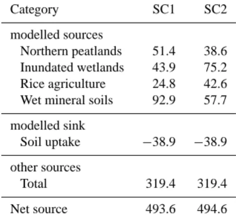
Table 2. Total global CH4 sources and sinks in 2004 (in

Tg CH4yr−1) simulated with LPJ for scenarios SC1 and SC2.

Other sources include anthropogenic emissions (EC-JRC/PBL, 2009), oceanic and geologic emissions (Lambert and Schmidt, 1993; Etiope et al., 2008; Neef et al., 2010) and emissions from termites (Sanderson, 1996). Category SC1 SC2 modelled sources Northern peatlands 51.4 38.6 Inundated wetlands 43.9 75.2 Rice agriculture 24.8 42.6 Wet mineral soils 92.9 57.7 modelled sink

Soil uptake −38.9 −38.9 other sources

Total 319.4 319.4 Net source 493.6 494.6

other sources is 319 Tg yr−1_{for the year 2004 for both} sce-narios (Table 2).

We did not include aerobic CH4 emissions from plants

(Keppler et al., 2006) in our study as they are likely to

con-tribute only 0.2–1.0 Tg CH4yr−1 to the global CH4 budget

(Bloom et al. (2010) and reply to comment by F. Keppler in Spahni et al., 2011). After the completion of our simulations,

another new source of CH4 emissions was found, namely

emissions from tank bromeliads in the canopy of tropical montane forests (Martinson et al., 2010), who estimated that about 1.2 Tg CH4yr−1are emitted from this source. In our opinion, this small source would have had no significant im-pact on the outcome of our study. We would like to note

that what is claimed to be a new source of CH4emissions by

Gauci et al. (2010) and Rice et al. (2010), is in fact implicitly included in our modelling approach of “naturally inundated wetlands” and “wet mineral soils”. Our modelling approach, as others before (e.g. Christensen et al., 1996) relate CH4 fluxes to heterotrophic respiration and soil moisture without

assuming any specific transport pathway; CH4may escape

via diffusion, ebullition or plant-mediated transport.

There-fore, we did not omit this potentially large source of CH4

emissions.

4 Results

Results of this study are twofold. First, we highlight the

re-sults of the biogeochemical modelling of natural net CH4

exchange using the LPJ dynamical global vegetation model. Second, we incorporate the natural net emissions together with estimates of anthropogenic emissions as prior fluxes into the atmospheric inversion systems TM5-4Dvar and

LMDz-SACS. The inversions provide corrections to the prior fluxes in time (both), space (both), and by category (TM5-4Dvar only). These corrections in turn help to validate and interpret the biogeochemical process model and constrain the two emission scenarios.

4.1 Biogeochemical process modelling

CH4emission strength as modelled by LPJ depends directly

on the global tuning parameter rC[CH₄]/C[CO2]for each wet

ecosystem type. While the soil HR is influenced by cli-mate and vegetation dynamics, rC[CH₄]/C[CO2]is assumed to

be constant over time and space. Setting rC[CH4]/C[CO2] for

the source types of peatlands, naturally inundated wetlands, rice agriculture and wet mineral soils, not only scales the CH4 fluxes per m2, but also impacts the latitudinal

distri-bution and global total of natural CH4emissions. Since the

attribution to different source types is quite ambiguous on a global scale, we propose two scenarios that satisfy regional

averages of local flux rates and the global CH4budget

(Ap-pendix A). These two criteria put a constraint on the param-eters rC[CH4]/C[CO2]for SC1 and SC2, which are given in

Ta-ble 1 and lead to global fluxes as given in TaTa-ble 2. SC1 is a scenario with large emissions from boreal peatlands and wet mineral soils. Emissions from naturally inundated wet-lands and rice agriculture are comparatively small.

North-ern peatland CH4emissions are calculated directly from an

initial version of Wania et al. (2010a). Soil uptake is calcu-lated directly from LPJ model output and the uptake scheme by (Curry, 2007). In SC2 emissions are dominated by natu-rally inundated wetlands (+70 % compared to SC1) and rice agriculture (+70 %) in the tropics and sub-tropics (Fig. 3). Peatland emissions (−25 %) and wet mineral soil emissions (−38 %) are substantially reduced in SC2. As a consequence the two scenarios mainly differ in latitudinal gradient of emissions and hence gradient of atmospheric concentration, but not as much in the seasonal cycle.

Highest net CH4exchange is simulated in the tropics (SE

Asia, Central Africa, South America) and the boreal regions (Siberia, Scandinavia, Eastern Canada, Alaska) as shown in Fig. 3. Beside these high-emission regions, the model

sug-gests large areas, where CH4 is emitted at a much smaller

rate (Fig. A1), predominantly at low latitudes. Figure 4a highlights the seasonality of emissions for different latitu-dinal bands. Highest net exchange on a global scale occurs from July until September, consistent with other studies (e.g., Chen and Prinn, 2006). The largest seasonal amplitudes are

simulated within the tropical bands of −30◦ _{to 0}◦ _{and 0}◦

to 30◦N. For these bands the emissions start increasing in

spring of each hemisphere. The total tropical emissions are largest for northern summer showing the dominance of the higher percentage of land area in the northern tropics. For the bands further north, the seasons start later, are shorter and contribute less to the global amplitude. This finding very much depends on the distribution of source areas that

Fig. 3. Net CH4emissions at 1◦×1◦resolution during (a) March

and (b) September 2004 in Gg CH4 per grid cell and month for

SC2. Net CH4 emissions are calculated as the sum of northern

peatlands, inundated wetlands, rice agriculture and wet mineral soil emissions minus soil uptake weighted by their grid cell fraction and area. Total global emissions from these sources and sinks in 2004 are 175.2 Tg CH₄.

are used in the calculation of total fluxes. As mentioned in Sect. 3, these areas are based on the organic soil carbon map for peatlands, the satellite data of inundated areas for naturally inundated wetlands and simulated soil moisture for wet mineral soil emissions and soil uptake. The impact of these distributions of both scenarios are shown in the bottom plot of Fig. 4b. Highest fluxes with ∼7 Tg CH4yr−1per de-gree latitude are found around the Equator. High fluxes over a broader latitudinal range are also found over the sub-tropics and the northern high latitudes. Both distributions modelled by LPJ are very similar to the latitudinal distribution jointly

estimated from SCIAMACHY CH4concentrations and

grav-ity space borne data by Bloom et al. (2010). The latitudinal

distribution of simulated CH4 fluxes (Fig. 4b) shows only

small year-to-year variability, which is understandable since in this study emissions from peatland and inundated wet-land areas only vary seasonally and not interannually. It has

been shown that both emissions per m2and emission areas

may vary independently, and total CH4emission variability

in space and time is regulated by both (Ringeval et al., 2010). A remarkable deviation from the latitudinal distrubtion es-timated by Bloom et al. (2010) is found at high latitudes,

where LPJ emissions peak between 50–60◦N and 60–70◦N;

the latter peak can not be constrained by the SCIAMACHY observations due to the instrument’s limited viewing geome-try. Large peatland areas existing north of 60◦N in Alaska, Scandinavia and the Western Siberian Lowlands (WSL alone

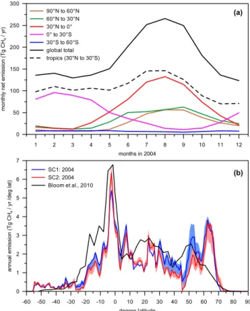
SC1: 2004 SC2: 2004 Bloom et al., 2010 -60 -50 -40 -30 -20 -10 0 10 20 30 40 50 60 70 80 90 degree latitude 0 1 2 3 4 5 6 7 an nu al e m is si on ( T g C H4 / yr /d eg la t) 1 2 3 4 5 6 7 8 9 10 11 12 months in 2004 0 50 100 150 200 250 300 m on th ly n et e m is si on ( T g C H4 / yr ) 90°N to 60°N 60°N to 30°N 30°N to 0° 0° to 30°S 30°S to 60°S global total tropics (30°N to 30°S) (a) (b)

Fig. 4. (a) Zonally integrated monthly net CH4emissions of 6

lati-tudinal bands and the global total for SC2 in the year 2004. Net CH4

emissions are calculated as the sum of northern peatlands, inundated wetlands, rice agriculture, and wet mineral soil emissions minus soil uptake weighted by their grid cell fraction and area. (b) Latitudinal distribution of annual net CH₄emissions for SC1 and SC2 in 2004, in comparison with methane emissions estimated from methane and gravity spaceborne data for the 2003–2005 average (Bloom et al., 2010). The colour shaded areas represent the 2 σ band of the inter-annual variability over the last two decades for the corresponding scenario.

is ∼592 440 km−2; Sheng et al., 2004) seem to contribute

to high latitude CH4emissions in LPJ. The atmospheric

in-versions presented in the next section show that these high-latitude peatland emissions are not in disagreement with

at-mospheric CH4 concentration data, though the inversions

suggest a reduction in their overall size.

4.2 Atmospheric inversion modelling

We apply the LMDz-SACS and TM5-4Dvar atmospheric in-version systems constrained by the observed atmospheric

CH4concentrations over the years 2003–2005 with an

em-phasis on the analysis for the year 2004. Since only the

TM5-4DVar system optimises CH4 fluxes by individual source

types, we use this system first to evaluate the two emission scenarios SC1 and SC2 (simulated by LPJ for the year 2004) against the observations. The prior differences between the

SC1 SC2

Fig. 5. Global CH4 budget prior (inner circles) and posterior

(outer circles) optimisation by the atmospheric concentration in-version using TM5-4Dvar. Emissions by category are given as rounded percentages of total emissions for SC1 and SC2 in the year 2004. The optimisation increased total gross emissions from 533 to 574 Tg CH4yr−1. Global sinks are not included in the diagrams.

two scenarios, in terms of individual sources and sinks, are

outlined in Table 1. The prior and posterior (optimised)

relative contributions per source type are shown in Fig. 5 for both scenarios. During the optimisation global gross emis-sions increase from 533 to 574 Tg CH4yr−1, and the relative source contributions change as well.

In Fig. 5 it can be seen that the relative strength of anthro-pogenic (∼55 %; coal mining, oil & gas, ruminants, biomass burning, waste and rice) to natural emissions (∼45 %; inun-dated wetlands, wet mineral soils, northern peatlands, ter-mites, and ocean and geologic) is not strongly affected by the optimisation. However, the source distribution within these large categories changes under optimisation. For

an-thropogenic sources, e.g., CH4 emissions are shifted from

oil and gas (−4 %) to increased emissions from ruminants (+6 %) and waste (+1 % to +2 %). Table 3 shows that the changes for the individual categories are substantial in ab-solute values. The optimisation also considerably reduces the associated error by 51 % and 29 % for oil and gas and ruminants, respectively. The transfer of emissions from oil and gas to domestic ruminants seems to be largely due to the difference in where these sources are on the planet: oil and gas emissions are heavily located in the Northern Hemi-sphere (e.g. Russia / Siberia), while domestic ruminant emis-sions are strong in South America. Focusing only on anthro-pogenic categories, the shift from oil and gas to ruminants largely reflects the increase in tropical / southern hemisphere emissions required by the inversion.

In regard to the natural sources, the optimisation affects

mainly northern peatlands. Peatland CH4emissions are

re-duced from 10 % to 5 % in SC1 and from 7 % to 5 % in

SC2. The opposite is true for CH4emissions from wet

min-eral soils and inundated wetlands (including rice agriculture). Although the relative contribution of emissions from these source types differ substantially between SC1 and SC2, the difference is preserved in the optimisation. This means that the inversion can not clearly differentiate between emissions from wet mineral soils or inundated wetlands. Emissions

Table 3. Regional total (anthropogenic+natural) emission changes

following the optimisation of the LPJ (SC2) scenario using TM5-4Dvar for the year 2004 at a 1◦×1◦resolution. Given are prior and posterior total fluxes by region (top) and category (bottom) in Tg CH4yr−1, their associated error and the estimated

uncer-tainty reduction. The 13 land regions are given as defined in the TRANSCOM3 model intercomparison experiment (Gurney et al., 2002), while the 14th region, referred to as “Oceans”, combines the 10 oceanic regions of TRANSCOM3.

Region Prior. emis. Post. emis. Prior. error Post. error Uncert. red.

Canada 18.3 13.3 1.7 1.5 14 % USA 32.4 51.3 4.0 2.2 46 % Central America 26.2 36.2 2.4 2.1 13 % South America 57.2 83.1 5.0 2.5 50 % NH Africa 36.9 55.0 3.1 2.8 12 % SH Africa 20.4 29.2 4.9 2.1 58 % Europe 66.7 52.4 7.5 3.1 59 % Siberia 35.0 27.7 4.9 2.2 56 % Arabia 12.0 10.2 4.7 1.7 63 % South Asia 59.3 45.8 8.0 3.2 60 % East Asia 64.2 73.2 6.3 3.0 51 % Australia 6.9 9.4 1.0 1.0 2 % Tropical Asia 30.8 33.7 2.4 2.2 9 % Oceans 28.4 27.8 1.4 1.3 5 % Globe 494.6 548.3 17.6 6.0 66 %

Category Prior. emis. Post. emis. Prior. error Post. error Uncert. red.

Coal mining 31.7 36.6 6.6 4.5 32 %

oil and gas 68.8 52.8 9.4 4.6 51 %

Ruminants 97.1 135.4 9.1 6.4 29 %

Biomass burning 26.9 27.7 3.3 1.8 44 %

Waste 60.4 68.2 6.1 5.2 15 %

Inundated wetlands 75.2 80.4 3.5 3.0 12 % Wet mineral soils 57.7 63.2 2.4 2.3 5 % Northern peatlands 38.6 28.2 3.0 2.2 28 % Rice agriculture 42.6 44.0 3.1 2.6 17 %

Termites 17.8 22.7 1.6 1.5 2 %

Ocean & geo 16.7 14.9 1.0 1.0 2 %

Soil uptake −38.9 −25.8 2.7 2.6 4 %

Globe 494.6 548.3 17.6 6.0 66 %

from these two categories have a large spatial overlap, such that after transport in the atmosphere, surface concentrations and satellite measurements can not help to distinguish be-tween them.

However, the inversion produces additional information on the spatial pattern for the LPJ simulated net exchange.

Fig-ure 6 shows the change in CH4emissions and uptake,

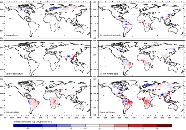
follow-ing optimisation, at grid cell resolution. Fluxes from north-ern peatlands are reduced in Scandinavia, Canada and Alaska (Fig. 6a), and tropical emissions (inundated wetlands, rice agriculture, wet mineral soils) are greatly reduced in Western South America, Bangladesh-India and Indonesia (Fig. 6b– d). On the other hand, the optimisation suggests a net in-crease in Eastern South American and Central African emis-sions. The latter is partly achieved by a reduction in soil uptake (from 39 to 26 Tg CH4yr−1globally, Fig. 6e). Emis-sion changes for the optimisation of SC2 are given in Ta-ble 3 for each category and for each geographical region, as defined in the TRANSCOM3 model intercomparison ex-periment (Gurney et al., 2002). It can be seen from

Fig. 6. Map of emission difference (Gg CH4gridcell−1yr−1) of fluxes before and after optimisation for the LPJ scenario SC2 in 2004

using TM5-4Dvar. Fluxes represent changes in the net exchange of the LPJ categories: (a) northern extra-tropical peatlands, (b) naturally inundated wetlands, (c) rice agriculture, (d) wet mineral soils, (e) soil uptake (positive numbers indicate a smaller uptake) and (f) sum of all fluxes (compare to Fig. 1).

relatively spread out over various regions, but with strong re-ductions/increases in particular regions. Regions with a large relative increase are the North American temperate and the North African region, while emissions from the Eurasian bo-real region are strongly decreased. Note that the regional

adjustments in Table 3 are for the total CH4 emissions per

region and thus also include substantial changes in anthro-pogenic sources (Fig. 5). As mentioned above, most impor-tant are increased emissions from ruminants (+40 %), mostly confined to North-and South America and decreased emis-sions from oil and gas industry (−23 %) mostly confined to Eurasia. Regional changes in anthropogenic emissions as de-rived from TM5-4Dvar inversions using surface and

SCIA-MACHY CH4observations have recently been presented by

Bergamaschi et al. (2009). Table 3 also shows the globally integrated uncertainty reduction of the inversion per emis-sion category. Although, the overall reduction in uncertainty is considerable (66 %), the atmospheric inversions can only give us estimates of how the LPJ fluxes should be corrected. The observations on its own are not a strong enough con-straint to distinguish between all sources, because they have significant spatial overlap. As a result from the inversion both scenario seem to be consistent with the observational constraint.

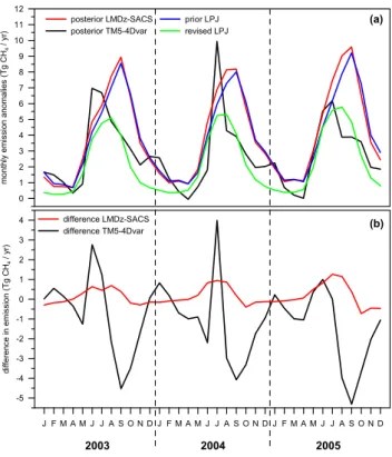
In summary, the strongest constraint imposed by the obser-vations on the LPJ-derived source and sink fluxes is the con-sistent reduction on northern peatland emissions in both sce-narios, SC1 and SC2, to about 5 % of total emissions (Fig. 5). Therefore, we evaluate the temporal evolution of northern peatlands over the years 2003–2005, using TM5-4Dvar and additionally using the LMDz-SACS inversion system. The evolution of monthly peatland emission anomalies over this time is shown for the prior, and the two posterior, emission estimates (resulting from the two inversions) in Fig. 7. The two inversions show quite large differences in the seasonality of posterior CH4fluxes, both being consistent with the atmo-spheric concentrations. While the LMDz-SACS-optimised posterior emissions have a similar seasonal duration to the prior fluxes, the TM5-4Dvar-optimised posterior emission season is considerably shorter. The difference between the inversion systems is inherent to their set-up. Temporal cor-relations in TM5-4Dvar are category-dependent and are not being applied to seasonally varying emissions such as from the peatlands at high northern latitudes. In LMDz-SACS the total of all sources is constrained over eight-day periods, with no time correlation between these periods. The discrepancy in the results clearly show how uncertain seasonal fluxes by inversions are. On the other hand, both inversion re-sults have a maximum correction in July and reductions in

J F M A M J J A S O N D J F M A M J J A S O N D J F M A M J J A S O N D -5 -4 -3 -2 -1 0 1 2 3 4 di ffe re nc e in e m is si on ( T g C H4 / yr ) difference LMDz-SACS difference TM5-4Dvar posterior LMDz-SACS posterior TM5-4Dvar prior LPJ revised LPJ 0 1 2 3 4 5 6 7 8 9 10 11 12 m on th ly e m is si on a no m al ie s (T g C H4 / yr ) 2003 2004 2005 (a) (b)

Fig. 7. Simulated CH4emissions from northern extra-tropical (45–

90◦N) peatlands for the years 2003–2005. Shown are priori emis-sions as calculated in LPJ and posterior emisemis-sions that have been optimised by atmospheric inversions with LMDz-SACS and TM5-4Dvar. Emissions are shown as absolute values (a) and as the differ-ence of inverison results to the prior (b). The revised LPJ CH4

emis-sions are obtained after including a more sophisticated parametrisa-tion of the CH4ebullition transport in the LPJ model (Wania et al.,

2010b).

August–October (Fig. 7b). This suggests that northern peat-land emissions apparently reach their maximum about one month earlier than simulated by LPJ.

The reasons for this disagreement between LPJ and the emissions inferred from observation by inversion lies in the separation of the three different pathways for CH4to escape

to the atmosphere. In LPJ, CH4 fluxes from plant

medi-ated transport and diffusion are highest in July, while ebul-lition fluxes from peatlands peak late in the season,

caus-ing the overall CH4 emissions to wrongly peak in

Septem-ber/October. In a revised version of LPJ we change the

parametrisation of the ebullition, such that all excess CH4

is emitted immediately and at a lower threshold, leading

to higher ebullition during summer. In the final version

of the model (Wania et al., 2010b), simulated CH4 fluxes

were recalibrated against site data using this new ebullition parametrisation. The recalibration results in slightly different model parameters, among which rC[CH4]/C[CO2] is reduced

from 20 % (SC2) to 10 % (Wania et al., 2010b). As a

conse-quence peatland CH4emissions are strongly reduced (from

38.6 to 25.6 Tg yr−1) and the new ebullition parametrisation

leads to a shift in seasonality. The revised LPJ seasonal emis-sions now have an improved time correlation with the TM5-4Dvar inversion results, where as before it was closer to the LMDz-SACS inversion results (Fig. 7). It is expected, that new inversions of the revised LPJ peatland emissions would lead to the same results.

4.3 Interannual variability

For the analysis of the interannual variabilty we set up an LPJ simulation using the new ebullition parametrisation and force it with the CRUNCEP reanalysis data set over the ex-tended period 1990–2008. Due to the new model setup an-nual fluxes differ from values in SC1 and SC2. Therefore,

we directly impose an agreement of the simulated CH4

ex-change with the TM5-4Dvar inversion budget in 2004 (Ta-ble 3) by scaling LPJ parameters and thus linearly scal-ing emission patterns for each category: northern peatlands

(from 25.6 to 28.2 Tg yr−1_{in 2004; ×1.10), inundated}

wet-lands and rice (98.9 to 124.4 Tg yr−1_{; ×1.26), wet mineral} soils (48.7 to 63.2 Tg yr−1_{; ×1.30) and soil uptake (−32.6} to −25.8 Tg yr−1; ×0.79). The scaling is explained for e.g. inundated wetlands and wet mineral soils by a change in parameter rC[CH4]/C[CO2] (Table 1) to values of 5.37 % and

0.67 %, respectively. Although, the individual source and sink attribution changes with the scaling, the impact on the interannual variability of simulated LPJ emissions is compa-rably small (see online replies to Spahni et al., 2011).

Using the LPJ emissions calibrated for 2004 we assess the

interannual variability in the simulated CH4 exchange due

to variations in the CRUNCEP climate input data. In Fig. 8

the LPJ-simulated CH4fluxes in natural ecosystems

(includ-ing rice agriculture) for the period 1990–2008 are compared to long term atmospheric synthesis inversions (updated from Bousquet et al., 2006), climate input variables and other LPJ output. Two apparent features are emerging. First, LPJ based natural ecosystem CH4emissions (including rice agriculture) increase over the 1990s and beyond (Fig. 8a). This partially agrees with the trends derived from atmospheric synthesis in-versions for global wetlands, with either constant or variable OH fields (updated from Bousquet et al., 2006). Second, the calculated anomaly (12 month running mean) of CH4

exchange of LPJ is smaller (± 7.1 Tg CH4yr−1) than the

inversion estimate (± 10.6 Tg CH4yr−1 with constant and

±11.5 Tg CH4yr−1 with variable OH). The LPJ emission

variability mainly reflects the variability of local fluxes due to climate variability and does not incorporate the variability of source area. Including this variability for naturally inundated wetlands for the years 1993–2000 (Prigent et al., 2007), the largest natural source of the LPJ categories, leads to a signif-icantly different evolution of interannual emissions (Fig. 8a). Its variability is larger and the trend is negligible. This result confirms the finding of Ringeval et al. (2010) who show that the source area variability and flux variability for inundated

CRUNCEP temperature (T) CRUNCEP precipitation (P) CRUNCEP 0.3._{T+ 0.7}._P 1990 1992 1994 1996 1998 2000 2002 2004 2006 2008 years -100 -80 -60 -40 -20 0 20 40 60 80 100 no rm al is ed in de x LPJ soil moisture LPJ heterotrophic respiration LPJ CH4 emissions -18 -15 -12 -9 -6 -3 0 3 6 9 12 15 18 an nu al e m is si on a no m al ie s (T g C H4 / yr )

LPJ inundated wetlands and rice agriculture LPJ wet mineral soils

LPJ northern peatlands LPJ soil uptake LPJ total -30 -25 -20 -15 -10 -5 0 5 10 15 20 25 an nu al e m is si on a no m al ie s (T g C H4 / yr ) LPJ

LPJ variable source area

update of Bousquet et al., 2006 (variable OH) update of Bousquet et al., 2006 (constant OH)

(a)

(b)

(c)

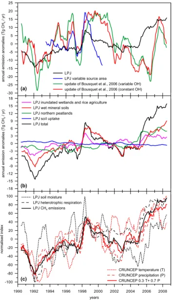
Fig. 8. Interannual variability in methane emissions. A centered

12-month running mean filter has been applied to smooth 12-monthly out-put. (a) Global CH₄emission anomalies simulated by LPJ (natural ecosystems and rice agriculture) for scenario SC2 are compared to synthetic inversion results for global wetlands updated from Bous-quet et al. (2006). “LPJ variable source area” denotes emission anomalies for 1993–2000 calculated by using the observed monthly inundated area (Prigent et al., 2007). (b) Simulated methane emis-sions by categories. The negative trend in soil uptake fluxes means more uptake with time. (c) Trends and variability in normalised en-vironmental variables. Shown are soil moisture and heterotrophic soil respiration simulated by LPJ, CRUNCEP temperature and pre-cipitation averaged over land and a linear combination of the latter.

wetlands are not necessary linearly related, and both are im-portant for CH4emission variability.

In our approach the LPJ emission variability is composed of the different source and sink categories (Fig. 8b). Emis-sions from northern peatlands and naturally inundated

wet-lands have a similar, but anti-correlated contribution to total source variability. Emissions from wet mineral soils show a larger variability and explain most of the total interannual variability. This can be partly explained by the soil moisture content. Its variability not only affects the CH4fluxes, but also the source area of wet mineral soils. However, areas of northern peatlands and inundated wetlands are not directly related to soil moisture availability in our study. Soil uptake has a comparably small variability, but is steadily increas-ing and thus slightly compensatincreas-ing the trend in emissions.

The main reason for the increase in total CH4emissions is

an increase in LPJ heterotrophic respiration. HR and CH4

emissions are highly correlated (R2=0.91). CH4emissions

go along with increasing temperature (R2=0.55) and

pre-cipitation (R2=0.83) over land as shown in Fig. 8c. Soil

moisture content alone is not well correlated to CH4

emis-sions (R2=0.22). A good predictor for the simulated global

CH4emissions is a normalised index that combines global

mean surface temperature (30 %) and global mean

precipita-tion (70 %) over land, favouring high CH4 emissions under

warm and wet conditions (R2=0.94).

5 Discussion

5.1 LPJ scenarios and budgets

Constraining natural CH4 emissions on a global scale has

several main components. Observational data on the

lo-cal slo-cale (flux measurements) and large slo-cale (global net-works, satellite data and mapping) in our analysis provide

the boundary conditions necessary to model CH4 fluxes at

intermediate scales. LPJ further constrains emissions by

simulating the biogeochemical processes. The inversion

systems then constrain emissions by calculation of

atmo-spheric transport and CH4 loss from the observed

atmo-spheric CH4concentration distribution. Despite these

vari-ous observational and modelling constraints, there remains more than one solution for the global source and sink dis-tribution. Finding “the optimal solution” certainly takes a

lot of effort at all scales. In this study we present two

LPJ emission scenarios, SC1 and SC2 (Table 1, Table 2, Fig. 5) that are evaluated. Northern peatland emissions for both scenarios are within the range of earlier estimates of

31 to 106 Tg CH4yr−1 (Zhuang et al., 2004). Yet, our

at-mospheric inversion results suggest northern peatland emis-sions being even lower than SC2 (39 Tg CH4yr−1) in 2004, at about 28 Tg CH4yr−1. This is in line with an earlier inver-sion study (Chen and Prinn, 2006), in which a prior estimate

of 43 ± 65 Tg yr−1for Northern Hemisphere emissions was

reduced to 33 ± 18 Tg CH4yr−1. This study also estimated

223 Tg yr−1 for remaining wet ecosystem methane sources

(including rice agriculture), which is more or less in line with our estimate of 204 Tg yr−1.

A decreased northern source asks for a compensation in other sources. Tropical sources have already been increased

from SC1 to SC2 by a 70 % larger carbon conversion rate rC[CH4]/C[CO2](tuning parameter) for natural inundated

wetlands and rice agriculture. Since the two categories

use the same parametrisation, an additional increase in

rC[CH4]/C[CO2], as suggested by the TM5-4Dvar inversion,

leads to slightly larger CH4 emission from rice agriculture

(Fig. 2). This limits CH4 emissions from inundated

wet-lands from 45◦N to 60◦S to ∼80 Tg yr−1. Additionally, wet mineral soils contribute ∼50 Tg CH4yr−1summing to a total of ∼130 Tg CH4yr−1in this latitudinal band. A separation of these two source categories by the inversion results has proven to be difficult. Overall, the reduced northern peatland source in SC2 compared to SC1 and the good agreement with emissions from rice agriculture, suggests that SC2 is a more plausible scenario than SC1.

Total natural ecosystem sources (171.5 Tg CH4yr−1) and the soil sink (38.9 Tg CH4yr−1) of SC2 in 2004 result in a prior estimated net soil source of 132.6 Tg CH4yr−1 (no rice agriculture). Using optimised fluxes from the TM5-4Dvar inversion based on SC2 (Table 3), net emissions yield

145 Tg CH4yr−1in 2004. Both estimates are in agreement

with the 145 ± 25 Tg CH4yr−1estimated by Chen and Prinn

(2006) for the years 1996–2001 and 137 ± 15 Tg CH4yr−1

estimated by Bousquet et al. (2006) for the years 1984– 2003. The “bottom-up” estimate for LPJ emissions scaled to 2004 inversion results (Fig. 8b) yields an average of 147 Tg CH4yr−1and a variability of ± 7 Tg CH4yr−1 over the years 1990–2008.

5.2 LPJ trends

All natural LPJ flux categories show an increase over the

years 1990–2008 (Fig. 8b) that becomes +1.03 Tg CH4yr−1

without rice emissions and +1.11 Tg CH4yr−1 when rice

emissions are included. The increase in simulated CH4

emis-sions is attributed to enhanced soil respiration resulting from the observed rise in land temperature and in atmospheric carbon dioxide that were used as input. With a conversion

factor of 2.78 Tg CH4ppbv−1and no change in atmospheric

loss this implies an atmospheric CH4 increase of 0.37 and

0.4 ppbv yr−1, respectively, which is very small and about the observed atmospheric growth rate for 2000–2006 (Dlu-gokencky et al., 2009). This trend does not support the hy-pothesis that natural wet ecosystem sources are fully respon-sible for the decline in the atmospheric growth rate since 1990. However, the increase in global emission fluxes could have been modulated or compensated by a decrease in global wetland area (Prigent et al., 2007; Ringeval et al., 2010). An alternative explanation of the limited growth in

atmo-spheric CH4despite rising anthropogenic and natural

emis-sions could be an increase in the tropospheric OH loss over this time period in relation to changing atmospheric chem-istry following increases in air pollution (Dalsøren et al., 2009; van Weele and van Velthoven, 2010).

The last decade shows a clear temporal division in the CH4 emission trends simulated by LPJ. The period 1999–2004

shows a small decrease (−1.03 Tg CH4yr−1) in agreement

with atmospheric synthesis inversions (Fig. 8a) and conclu-sions by Bousquet et al. (2006), while the period 2005–

2008 shows a considerable increase (+3.62 Tg CH4yr−1,

Fig. 8a,b). This increase contributes to the observed maxi-mum in atmospheric growth rate in 2007 (Dlugokencky et al., 2009). The biggest contribution of the 2008–2004 difference

in simulated CH4emissions (17.33 Tg CH4) comes from wet

mineral soils (56.6 %). Northern peatland emissions (24.3 %) and emissions from inundated wetlands including rice agri-culture (20.5 %) contributed similarly, but less, to the rise in CH4. The LPJ run also suggests that only post 2005 are the inter-annual emission anomalies of peatlands and inundated wetlands not anti-correlated (Fig. 8b). The compensation of emissions through an increased soil sink is small (−1.4 %).

This source attribution agrees with the finding of Dlugo-kencky et al. (2009), namely that despite the emission in-crease at Arctic latitudes, the largest inin-crease in atmospheric

CH4concentrations in 2007 happened in the tropics. This

is represented in the simulation by the dominant contribution in 2006/2007 from the low-latitude sources wet mineral soils, inundated wetlands and rice agriculture (Fig. 8b). Emission fluxes could be modulated by variations in global wetland area, which is partly considered by the change in emission area of wet mineral soils that seem to play an important role

for the inter-annual CH4variability. The inclusion of a

hy-drological module in a DGVM, that calculates wetland area in addition to wetland fluxes, as well as more observational constraints are needed to properly address questions on long

term trends in global CH4emissions.

6 Summary and conclusions

In a multiple model approach we derive estimates for global

CH4emissions and uptake in organic and mineral soils that

are in agreement with atmospheric observations. We show

that the global CH4 source category usually summarised in

the literature as “wetlands” can be usefully broken down into process-defined subcategories: northern peatlands, naturally inundated wetlands, rice agriculture and mineral soils. Min-eral soils are mostly treated in the literature as a potential

CH4sink, but unsaturated mineral soils are also a potential

CH4source. Even if most of the produced CH4is oxidised

and fluxes per m2are relatively small, areas with moderately high soil moisture are very extensive and result according to our calculations, in gobal emissions of ∼60 Tg CH4yr−1. Natural CH4fluxes simulated by LPJ are scaled to global to-tals using fractional source area maps (Prigent et al., 2007; Global Soil Data Task Group, 2000; Leff et al., 2004). With

this global approach we find CH4emissions from rice

agri-culture in SE Asia in agreement with recent EDGAR inven-tory estimates (EC-JRC/PBL, 2009). The resulting global CH4emission distribution by latitude for the LPJ categories