Sedimentation of self-propelled Janus colloids: polarization and pressure

HAL Id: hal-02178326

https://hal.archives-ouvertes.fr/hal-02178326

Submitted on 9 Jul 2019

HAL is a multi-disciplinary open access

archive for the deposit and dissemination of

sci-entific research documents, whether they are

pub-lished or not. The documents may come from

teaching and research institutions in France or

abroad, or from public or private research centers.

L’archive ouverte pluridisciplinaire HAL, est

destinée au dépôt et à la diffusion de documents

scientifiques de niveau recherche, publiés ou non,

émanant des établissements d’enseignement et de

recherche français ou étrangers, des laboratoires

publics ou privés.

polarization and pressure

Félix Ginot, Alexandre Solon, Yariv Kafri, Christophe Ybert, Julien Tailleur,

Cécile Cottin-Bizonne

To cite this version:

Félix Ginot, Alexandre Solon, Yariv Kafri, Christophe Ybert, Julien Tailleur, et al.. Sedimentation of

self-propelled Janus colloids: polarization and pressure. New Journal of Physics, Institute of Physics:

Open Access Journals, 2018, 20 (11), pp.115001. �10.1088/1367-2630/aae732�. �hal-02178326�

Univ. Lyon, Université Claude Bernard Lyon 1, CNRS,UMR 5306, Institut Lumière Matière, F-69622, Villeurbanne, France 3 _{Department of Physics, Massachusetts Institute of Technology, Cambridge, MA 02139, United States of America} 4 _{Department of Physics, Technion, Haifa, 32000, Israel}

5 _{Université Paris Diderot, Sorbonne Paris Cité, MSC, UMR 7057 CNRS, F-75205, Paris, France} E-mail:cecile.cottin-bizonne@univ-lyon1.fr

Keywords: sedimentation, self-propelled colloids, polarization

Abstract

We study experimentally—using Janus colloids—and theoretically—using Active Brownian Particles

—the sedimentation of dilute active colloids. We first confirm the existence of an exponential density

profile. We show experimentally the emergence of a polarized steady state outside the effective

equilibrium regime, i.e. when the sedimentation speed v

s

is not much smaller than the propulsion

speed v

0

. The experimental distribution of polarization is very well described by the theoretical

prediction with no

fitting parameter. We then discuss and compare three expressions which have been

proposed to measure the pressure of sedimenting particles: the weight of particles above a given

height, the

flux of momentum and active impulse, and the force density measured by pressure gauges.

1. Introduction

The sedimentation of active particles has recently attracted a lot of interest, both experimentally[1,2] and

theoretically[3–10]. In the simplest of limits in which the interactions between particles can be neglected and

their sedimentation speed vsis much smaller than their self-propulsion speed v0, the system behaves as an

equilibrium one, leading to an exponential density profile

r( )z µexp(-mgz kTeff). ( )1 The effective temperature is then given by a Stokes–Einstein relation kTeff≡D/μ, with D and μ the diffusivity

and the mobility of the particles. This regime was observed experimentally for self-diffusiophoretic Janus colloids[2]. The impact of interactions between particles on the above small vs/v0regime was recently explored

experimentally and numerically in[1].

In this article, we consider experimentally and theoretically the fate of dilute active sedimenting systems when the sedimentation speed cannot be neglected, i.e. beyond the effective equilibrium regime. We use self-propelled Janus colloids in 2D as a model experimental active system, and model them using non-interacting Active Brownian Particles(ABPs, see section2). We first consider the distribution of particles in the

sedimentation profile (section3). Our experiments show that the gravity field leads to a polarized steady state in

agreement with earlier theoretical predictions[3,5,11]. Furthermore, the distribution of orientations of the

particles within the exponential sedimentation profile agrees quantitatively, without any fitting parameter, with the one predicted analytically for sedimenting ABPs[5].

The pressure of active particles has attracted a lot of interest recently[12–25]. We discuss the expression of

pressure for sedimenting active particles[1] (section4). For our ABP model, we give a clear interpretation of a

bulk pressure, defined as the weight exerted on the system above a certain height [1,26–30], in terms of

momentum transfer. We give a complete characterisation of the latter in terms of correlators measured in the bulk of the system and a recently introduced active impulse[14]. Excellent agreement is shown between

10 October 2018

PUBLISHED

6 November 2018

Original content from this work may be used under the terms of theCreative Commons Attribution 3.0 licence.

Any further distribution of this work must maintain attribution to the author(s) and the title of the work, journal citation and DOI.

experimental measurements of the pressure and these bulk observables. Finally, we discuss whether such an expression of pressure can be related to force densities exerted on pressure gauges.

2. Experimental setup and theoretical model

When immersed in a hydrogen peroxide(H2O2) bath, gold Janus colloids of radius a=1.1±0.1 μm half

coated with Platinum become active and propel themselves with a force f3_pDby self-diffusiophoresis[31]. Their

density being very high aroundρ=11 g cm−3, the colloids immediately sediment onto theflat bottom of an experimental cell to form a bi-dimensional layer of particles. Due to the huge reservoir of peroxide, activity can be considered as constant during each experiment. For each experiment we record movies of 5000 images @ 20 fps, for a total duration of 250 s. This experimental set-up, sketched infigure1, was previously used to study the cluster phase[32] and the weak sedimentation limit [1] of active Janus colloids.

Here, using a piezoelectric module, we tilt the experimental cell with an angleα to create a reduced gravity fieldg sina, leading to a controllable sedimentation velocity vs, that we take along the z-axis: -v es z. We start

with an angleα as small as possible, and we increase vsby increasingα, until all the gas collapses into the dense

phase. In the following we denotev u0 ( )q the 2D propulsion velocity of a colloid in the(x, z) plane (see figure1). Note that, experimentally, we measure the velocity of a particle at positionr:r˙=v0u( )q -vs ze . For each

experiment we measure v0, which is found around 4±0.2 μm s−1, and vs(see appendicesAandBfor details). In

the following, we will present experimental results for different realisations corresponding to values of the ratio vs/v0from∼0.08 to ∼0.28.

To account for our experimental results, we model the colloids as ABPs[33] that are self-propelled at a

constant velocity v0along their internal direction of motion u and subject to rotational diffusion. As in the

experiments, the motion of the particles is restricted to the 2D plane parallel to the bottom plate and subject to a sedimentation velocity -v es zdownward along the z-axis. Furthermore, we will assume that the orientation

vectors u of the particles are also restricted to this 2D plane. This is not the case experimentally since the propulsion force f3D_{p can point in any direction in 3D. However, we do not have experimental access to the 3D}

statistics of f3Dp and we show in appendixBthat allowing rotational diffusion in 3D for the ABPs leads only to

quantitatively similar results with small corrections, so that our experimental data are not able to distinguish between the two situations. For simplicity, we thus consider a propulsion velocity offixed norm v0and 2D

orientation vectoru( )q = -( sin , cosq q), subject to rotational diffusion with diffusion coefficient Dr. The

overdamped dynamics of a particle at positionrand with a sedimentation speed vsthen follows the Langevin

equation

q q x

= - =

˙ v ( ) v ˙ D ( )

r 0u s ze ; 2 r , 2

whereξ is a Gaussian white noise with zero mean and unit variance x xá ( ) ( )t t¢ ñ =d(t- ¢t . The persistence) timet ºp Dr-1and lengthlpºv D0 r-1provide natural time and length units. Numerically, we integrate

equation(2) using Euler time-stepping with time step dt=0.1τp.

Equation(2) does not include interactions between particles and thus only attempts to describe the dilute

gaseous phase of the experiments. It would be interesting to ultimately describe interacting particle systems, to be able to resolve the full sedimentation profile. This would require adding short-range pairwise forces to the dynamics in(2). It could also be interesting to study the role of inter-particle torques, even if nothing indicates

that these play an important role in our experimental setup. Then, the externalfield could induce external

Figure 1. Left: illustration of the experimental setup. Janus particles are immersed in a hydrogen peroxide bath and sediment towards the bottom of the experimental cell. They then form a monolayer where each particle moves with 2D velocityr˙resulting from both self-propulsion and sedimentation. Using a piezoelectric device we tilt the experimental cell by an angleα which leads to a reduced gravity_fieldg sin . Right: 2D scheme of a Janus particle under sedimentation. The particle moves forward with a mean velocity va 0and

torques on the particles, a topic which has been studied recently in[34]. Note finally that equation (2) does not

include thefluid which surrounds the colloids. The latter indeed rest on a tilted surface which acts as a local momentum sink, which legitimates neglecting the role of hydrodynamics in this setup6.

3. Sedimentation profile and polarization

The steady state distribution of sedimenting ABPs described by equation(2) is an exponential density profile

[3,5,6,11]. Indeed, the Fokker–Planck equation for the probability (r, ,q t)tofind a particle at positionr

with orientationθ at time t reads

  

¶t = -· [(v0u-vs ze ) ]+Dr¶_q2 , ( )3 and by symmetry (r,q)=(z,q). As shown in[5], equation (3) can be solved by separation of variables.

Writing P(z, θ)=f (θ)ρ(z) in equation (3), ρ and f satisfy in steady state

r¢( )z = -r( )z l, ( )4 q l q q ( )= - ( - ) ( )= ( ) f D v v f 1 cos 0. 5 r s 0

The density profile is thus of the form ρ(z)∝e−z/λ, with a sedimentation lengthλ. The solutions of equation(5) are Mathieu functions. The periodicity of f (θ) then implies [5]-4vs (lDr)=a0(-2v0 (lDr)) where a0is thefirst characteristic value of the Mathieu equation (see [35] for properties of the solutions of

equation(5)). Expanding a0for small vs/v0[35], one gets the sedimentation length λ as l = ⎡ - + ⎣ ⎢ ⎢ ⎛ ⎝ ⎜ ⎞ ⎠ ⎟ ⎛ ⎝ ⎜⎜⎛_⎝⎜ ⎞ ⎠ ⎟⎞ ⎠ ⎟⎟⎤ ⎦ ⎥ ⎥ ( ) v D v v v O v v 2 1 7 4 . 6 r s s s 02 0 2 0 4

At the same order in vs/v0, one gets for the orientation distribution: p q = + q+ q+ ⎛ ⎝ ⎜⎜⎛_⎝⎜ ⎞ ⎠ ⎟⎞ ⎠ ⎟⎟ ( ) ( ) f v v v v O v v 2 1 2 cos 2 cos 2 . 7 s s s 0 2 02 0 3 3.1. Density profile

Wefirst measure experimentally the density profile r( )z . To do so, we use a coarse graining operation(5.1 μm

height slices) and both a spatial average over the x-axis and a time average over the experiment duration. In figure2the resulting experimental sedimentation profiles are shown for several values of vs/v0. The density

profiles indeed exhibit an exponential decay in the dilute phase—which corresponds to a linear dependence in our semi-log plot—with a sedimentation length λ.

Figure 2. Left:ρ(z) for vs/v0=0.09, 0.13, 0.18, 0.29. We observe an exponential decay in the dilute gas phase, where particle

interactions become negligible. Note that for a better display the origin of z is arbitrary. The plain lines correspond to a joint_{fit of all} data sets with one free parameter, Dr, which is found to be Dr=0.08±0.003 s−1. Right: picture of the experimental system for

vs/v0=0.29. Blurry particles at the top are due to the defocus induced by the tilt of the sample.

6

The theoretical expression for the sedimentation length equation(6) depends only on parameters that

should be accessible experimentally. However, measuring precisely the rotational diffusion coefficient Drof the

active colloids is difficult. The statistics of the velocity autocorrelation in the dilute gas region is indeed too limited to accurately measure Dr. Therefore, we use Dras a free parameter andfit the density profiles shown in

figure2with equation(6). This leads toDr=0.080.003 s-1. Note that this value is compatible with the Brownian estimate Dr=0.12±0.04 s−1(the significant errorbar is due to 10% polydispersity). Our slightly

smaller measurement could be due to the proximity of the bottom surface. 3.2. Polarization

A remarkable feature of the sedimentation profile of active particles is the existence of a non-vanishing mean polarization. Afirst visualisation of this polarization can be obtained from the distribution of velocities in the sedimentation profile. We measure the instantaneous velocities of free particlesr˙—positions are smoothed with

a Gaussian average over s1 , particles are considered free if they have no neighbour in a radius of 5.1μm—and build the corresponding 2D probability distribution function(see figure3). Note thatr˙corresponds to the observed velocity, which includes both the propulsion velocity v0u(θ) and the sedimentation velocity −vsez.

As expected, when the sedimentationfield is negligible, for example when vs/v0∼ 0.09, the distribution of

velocities has an isotropic‘ringlike’ shape, with a radius∼v0. On the contrary, when the sedimentation speed

increases, a striking behaviour emerges as the microswimmers polarise against the gravityfield: the distribution of velocities is no longer isotropic and colloids are most likely oriented upwards, leading to a strong peak of probability at the top of the ringlike distribution. Note that, due to the sedimentation velocity, there is also a downward shift of the centre of the ring, which is clearly visible when vs/v0is large enough.

To compare with theoretical predictions based on the ABP model(2), we extract the orientation

distribution f( )q from the experimental 2D probability distribution of˙r(see appendixA). We plot the

orientation distribution 2πf (θ) in figure4(symbols) against the theoretical prediction from equation (7) (solid

lines). Note that the agreement between experiments and theory is remarkable, without any fitting parameter. Modelling our self-propelled Janus colloids as ABPs thus allows us to quantitatively account for their

sedimentation profile.

4. Pressures in sedimentation pro

files

Studying the pressure of active systems is a fascinating challenge for at least two reasons:first as the out-of-equilibrium fate of a thermodynamic state variable that controls phase equilibria andflows in passive systems.

Figure 3. Probability distribution of the measured velocities˙r. The colour code corresponds to a normalised distributionP x z( ˙ ˙), . The polarization becomes more apparent as vs/v0increases. The downward offset of the distribution gives access to the sedimentation

Then as a measurement of the force that active particles collectively exert on their environment. Since active particles exchange momentum with the environment, their momentum does not satisfy a conservation equation so that pressure cannot be unambiguously defined from their momentum flux. In particular, such a bulk expression is not, in general, equivalent to the force density exerted by active particles on a confining boundary [20].

There are notable exceptions to this lack of equation of state, such as non-interacting ABPs[17,21,23,25].

For such models, a homogeneous isotropic system exerts a force density on a container that can be expressed as observables measured in the bulk of the system, despite wall-dependent boundary layers. The question as to whether this extends to our polarized sedimentation profile is completely open. (See [34] for the case of weak

sedimentation where the polarization can be neglected.) In section4.1, wefirst show that a pressure defined as the weight exerted on the active system above a certain height can be related to momentum transfer in the bulk of the system, as suggested in[1]. Nevertheless, we show in section4.2that this bulk pressure cannot be related to the force density measured by a confining interface: it cannot be read with a pressure gauge. The difference between such a mechanical measurement and our bulk pressure however vanishes as vs/v0→0, provided the

pressure gauge is oriented orthogonally to the gravityfield. 4.1. Pressure as momentumflux: the active impulse

In equilibrium, the equation of state relating the osmotic pressure to bulk properties of a system can be directly measured using a sedimentation profile [26,28], within a local density approximation. The underlying idea is

that the total weight exerted on the particles above a given height z is balanced by the osmotic pressure at this height so that the pressure can be measured as:

ò

r

P ( )z = ¥ mg ( )z¢ d ,z¢ ( )8

z

w eff

where mgeffis the effective weight of the particles. Within the local density approximation, one then infers

Πw(ρ(z)) from Πw(z). Equation (8) can be seen as a consequence of momentum conservation above a height z:

the incoming momentumflux, which we write Πm(z), is balanced by the total external force (density) applied

above a plane z,Πw(z), which is the only external source of momentum.

It is natural to ask whether this construction also applies to active systems, as recently proposed[1]. Indeed,

each active particle injects momentum into the activefluid so that momentum is not conserved. This injection of momentum can be quantified using the active impulse Dpa_{[14]. For particle i, at position r}

iand orientationθi,

Dp_ia_{measures the total momentum the particle will receive on average from the environment in the future:}

ò

Dp_i( )t = ¥ dsf ( )s , ( )9

t i

a p

wheref_ip=fpu( )qi is the propulsion force of the particle and the overbar represents an average over future

histories, forfixed ri(t) and θi(t). Interestingly, it was recently shown that a class of active systems, to which our

ABP model(2) belongs, admits a generalised conservation law: the sum of the particles’ momenta and of their

active impulses[14] form a conserved quantity. In such cases, one can show [14] that the active impulse

corresponds in steady-state to the swim pressure introduced in[23,25]. We now show that, in this context,

Figure 4. Distribution of particle orientations for increasing vs/v0=0.09, 0.13, 0.18, 0.29. Symbols correspond to experiments and

Πw(z), defined in equation (8), can be related to the flux of momentum and active impulse through an interface

at height z.

We consider particles evolving under the dynamics(2). The dynamics of the microscopic density field

rˆ = å_id(r-ri)is given by r = -ˆ˙ · ˆJ (10)

å

r q d º - + -ˆ _{v ˆ v ( ) ( ) ( )} J s ze u r r . 11 i i i 0

In a sedimentation profile, the steady state is flux-free leading to a vanishing mean current º á ñ =_J ˆ_{J 0, so that}

å

r( ) = á ( ) (q d - )ñ ( ) vs r ez v u r r , 12 i i i 0

where the angular brackets are steady-state averages and we have introducedrº á ñrˆ . Equation(12) simply states

that the downward contribution to the density current due to the sedimentation of the particles is opposed by an average upward bias of their active force orientations as already shown in the study of the polarization in section3. For non-interacting ABPs, the rhs of equation(12) can be rewritten as the flux of active impulse (see [14] and appendixD)

å

q d

å

m d á v u( ) (r-r)ñ = - á· r˙ Dp (r-r .)ñ i i i i i _i i 0 a

Integrating equation(12) from z to¥, projecting along ez, and dividing byμ then leads to

ò

r

å

d P ( )z = ¥ mg ( )z = á z˙Dp (r-r)ñ º P ( )z (13) z _i i z i i w eff , a m

whereΠm(z) is the upward flux of active impulse. Note that, here and thereafter, we retain the x-dependence in d(r-ri)for dimensionality reasons, even though the result solely depends on z. Equation(13) balances the total force exerted on the system above z, given by the lhs, with theflux of active impulse through the horizontal plane at height z. If we were to include a diffusive contribution to the dynamics(2), this balance would become

ò

¥ mg r( )z = á

å

z˙Dp d(r-r)ñ +rkT- ¶ áD

å

Dp d(r-r ,)ñ (14)

z eff _i i z i, i z _i z i i

a

, a

where the last two terms come from the diffusivefluxes of momentum and active impulse, respectively. The central result(13) shows that, rather surprisingly in this momentum non-conserving system, the total force density

applied above a height z,Πw(z), is balanced, as in equilibrium, by an upward effective momentum flux, Πm(z).

To make connection with our experimental system, we note that, for ABPs, the active impulse(9) can be

readily computed as[14] q D = f ( ( )) ( ) D t p pu . 15 r a

Rewriting(13) then leads to

å

å

m q d m q d P ( )z = v á ( ) ( - )ñ - á ( ) ( - )ñ ( ) D v v D r r r r cos cos . 16 r i i i s r i i i m 0 2 2 0

Introducing the orientation and nematicfields

å

q d = á - ñ ( ) ( ) ( ) ( ) m rz cos r r 17 i i i

å

q d = á - ñ ( ) ( ) ( ) ( ) Qzz r cos 2 r r , 18 i i i

which solely depend on z in the steady state, equation(16) can be rewritten as

m r m P ( )z = v [ ( )+ ( )]- ( ) ( ) D z Q z v v D m z 2 r . 19 zz s r z m 0 2 0

Equation(19) shows that, unlike in equilibrium, Πm(z) measured in a sedimentation profile, and thus Πw(z),

do not give access to the pressure of a bulk homogeneous system of densityρ0=ρ(z). Indeed, the latter would be

given by = _mv r

D

2 r 0

02

. The difference is due to the non-isotropic orientation of the active particles in the

sedimentation profile. Note that the local density approximation of the equilibrium case is here generalised into a new local approximation involving mzand Qzz, and not onlyρ(z). The fact that these two new fields are

different in sedimenting and homogeneous isotropic active systems is the reason why the EOS of the latter cannot be directly read from sedimentation experiments; it can however be reconstructed from the joint measurement ofΠw, mzand Qzz(provided v0, vs,μ and Drare known). Note that the difference between Πm(z)

andvanishes in the limit vs/v0→0, as expected in this effective equilibrium regime in which active particles

Using f(θ) computed in section3, one can rewrite mzand Qzzas r r = + ⎜⎛ ⎟ = + ⎜ ⎟ ⎝ ⎞⎠ ⎛ ⎝ ⎜⎛_⎝ ⎞_⎠⎞ ⎠ ⎟ ( ) ( ) ( ) ( ) ( ) m z z v v o v v Q z z v v o v v ; 4 20 z s s zz s s 0 2 02 2

so thatΠm(z) can be rewritten as:

m r P = ⎛ - + ⎜ ⎟ ⎝ ⎜ ⎛ ⎝ ⎜⎛_⎝ ⎞_⎠⎞ ⎠ ⎟⎞ ⎠ ⎟ ( )z v ( ) ( ) D z v v o v v 2 1 7 4 . 21 r s s m 0 2 2 02 2

For the experimental system described in section2we measure:

ò

mP ( )z =vs dzr( )z + Pm , (22) z w L out

where L corresponds to the top of the experimental observation box and

ò

mPout =vs ¥ dzr( )z . (23)

L

We extractμΠoutby plotting equation(22) against equation (21) for all accessible values of z (see appendixC).

We could equivalently use equation(19) but the measurements of Qzz(z) and mz(z) are noisier and the

corresponding estimate ofΠoutslightly less reliable. As shown infigure5, the agreement between the

experimental measurements ofΠw(z) and our theoretical predictions for Πm(z) is very good. This agreement is

quantified in figure6using a parametric plot. Finally, note that, in our experiments, the ratio vs/v0is large

enough to lead to a clear polarization of the sedimentation profile, as shown in section3. The correction to pressure due to polarization however scales as(vs/v0)2so that, although measurable, the impact of polarization

on the pressure measurement is limited(see figure6).

4.2. Connection to mechanical forces

In equilibrium, the relation between momentumflux and force densities exerted on confining interfaces is well understood. In particular the mechanical pressure, defined as the force density on a confining vessel, is equal to the hydrodynamic pressure defined from a bulk stress tensor so that the former satisfies an equation of state: it does not depend on the details of the confining potential. In active matter, on the other hand, the mechanical pressure is generically not given by an equation of state, except in exceptional cases to which our ABP model(2) belongs. It is

thus natural to wonder whether these results, obtained for bulk homogeneous systems, extend to the case of sedimenting profiles. Note that a complementary approach based on continuum mechanics can be found in [34].

To answer this question, we compare the‘bulk’ pressuresP ( )w z , defined inequation (8), and its expression

as an effective momentumflux, Πm, computed as equation(19), to the mechanical pressure felt by

(semi-permeable) pressure gauges. We first consider a pressure gauge modelled as a confining potential starting at height zw, invariant by translation along x, and confining the particles from above (see figure7). We thus

measure a force density along the ˆz axis, that we call Pz. We then turn to the complementary problem of a vertical

confining potential starting at xwand compute the corresponding force density Px(see figure7).

Figure 5. Pressure pro_{files for}v vs 0 = 0.29. In black, the pressureΠw(z) measured experimentally by integrating the density above

a height z, following equation(22). In blue, the effective momentum flux Πm(z) predicted by equation (19) and, in green, its

approximation equation₍21_{). Note that the curves for Π}mcorrespond to local measurements whereasΠw(z) results from an

Taking into account the confining potential Vw, the dynamics of the system becomes

q m

= - - 

˙ v ( ) v V ( ) ( )

r 0u s ze w r . 24

The mechanical pressure exerted by the particles on the confining gauge boundary can be computed as

ò

r

= ¥ ¶

( ) ( ) ( ) ( )

P zz w z V z d ,z 25

zb z w

where zbis any height in the bulk of the system, withzbzw. Note that the formula(25) is completely generic and

holds for any confining potential. It does not depend on the choice of zbsince Vwvanishes forzzw. Furthermore,

the convergence of the integral asz ¥is ensured by the fact that the density of particle vanishes in the wall. Using standard methods[20] detailed in appendixE, one gets that

m r m + = + -( ) ( ) [ ( ) ( )] ( ) ( ) P z W z v D z Q z v v D m z 2 , 26 z w w r w zz w s r z w 02 0

where we have introduced the weightW z( )=

ò

¥ mg r( )z dz

z eff of active particles above a given height z in the

presence of the confining boundary.

Crucially, comparing(19) with(26) shows that measuring the weight Πw(zw) of active particles above a

given height zwin an unbounded sedimentation profile (or the effective momentum flux Πm(zw) at this height) is

Figure 6. Parametric plot ofμΠm(z), equation (19), versus μΠw(z), equation (22), for vs/v0=0.29 (blue symbols). The black dotted

line y= x is a guide for the eye that corresponds to our theoretical predictions. A best affine fit y = ax + b gives a=1.04 and b=0.003. The role of polarization for this value of vs/v0can be visualised usingm= r( )z

v D 2 r

02 _{instead ofΠ}

m(red symbols), which

leads to a=1.16 and b = 0.001. The 1.16 prefactor corresponds to the prediction(21): -

(

1 v

)

1.17 v 7 4 1 s2 02

. Inset, parametric plot of the approximation(21) of μΠm(z) versus μΠw(z), which leads to a=0.99 and b=0.

Figure 7. Illustration of the measurements of the mechanical pressure defined as a force density exerted on a pressure gauge. Left: upon inserting a horizontal pressure gauge, the particles are confined from above. They start experiencing a repulsive potential when reaching a height zw. Right: the pressure gauge is now oriented along gravity. Particles start experiencing a repulsive potential when

which the free energy is extensive, which is not the case for sedimenting systems. That said, the weight(density) of passive particles interacting with the pressure gauge is of the order ofρmgσ, where σ is the interaction range of the confining potential; for non-interacting sedimenting particles, it has to be compared with a pressure ρkT so that the violation of the equation of state is measured byσmg/kT. This is the ratio between the range of the confining potential and the sedimentation height; for sedimenting colloidal particles, this would be completely negligible. On the contrary, for an active system, there is afinite boundary layer of particles that accumulate at the wall, which makes this contribution non-vanishing even whenσ → 0. Using standard results on the accumulation of active particles at confining boundaries [36], we find this contribution to be of the order of vs/v0

7

.

Let us now look at what happens for a confining boundary oriented normal to the ˆx direction (see figure7).

The exact same computation as above leads to

r m r = + + ( ) ( ) [ ( ) ( )] ( ) P z kT x z v D x z Q x z , 2 , , , 27 x b r b xx b 02

where(xb, z) corresponds to a point in the bulk of the system. Interestingly, this z-dependent force density

satisfies an equation of state, and will not depend on the details of the confining boundary. It is entirely predicted by bulk properties of thefluid, but, again, these properties are not measured by Πw(z), since(27) differs

from(19) because the fluid is anisotropic. Note that for weakly sedimenting systems, however, equation (21)

shows the difference between Px(z) and Πw(z) to vanish so that a pressure gauge could be used, in principle, to

accessΠw(z) or Πm(z) when the self-propulsion speed is much larger than the sedimentation velocity.

5. Conclusion

In this paper we have used active Janus colloids and ABPs to study sedimenting active particles. We have shown experimentally that when the sedimentation speed is comparable to the propulsion speed, a net polarization of the active colloids develops in the bulk of the system. The theoretical predictions for the distribution of orientations of the particles agree very well with the experimental results without any free parameter. We then discussed different expressions of pressure for sedimenting active particles. Using our ABP model, we have shown that the bulk pressure defined as the weight exerted on the system above a certain height can be interpreted in terms of local momentum transfer. This is verified to a very good approximation in our experiments. Finally we discussed when such bulk expressions of pressure can be related to local force densities exerted on pressure gauges.

Acknowledgments

YK is supported by an I-CORE Program of the Planning and Budgeting Committee of the Israel Science Foundation and an Israel Science Foundation grant. JT is funded by ANR Baccterns. JT & YK acknowledge support from a joint CNRS-MOST grant and the hospitality of MLB Center for Theoretical Physics.

Appendix A. Measuring

v

s

and maximum

v v

s 0

ratio

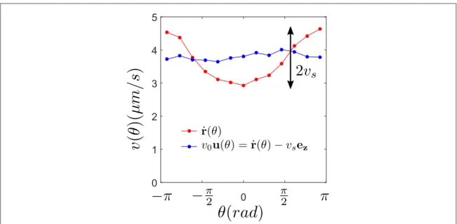
A.1. vsmeasurement

Getting a precise measure of vsis essential as we do not have direct access tov u0 ( )q but tor˙=v0u( )q -vs ze .

While we measure the tilt of the experimental chamber with the resultingα angle, and could apriori compute vs,

7

the resulting error bars are too large for a quantitative study. We thus decided to measure it aposteriori using the 2D probability density function, and the fact thatr˙ ( )0 -r˙ ( )p =2vs. This gives much more precise

measurement of vsand indirectly v0and f(θ). We verify in figureA1thatr˙ ( )q is not isotropic due to vs

contribution(red), but that as expectedv0u( )q = -r˙ vs ze becomes isotropic when we remove vs

contribution(blue).

A.2. Maximum v vs 0ratio

In the experiments the ratio vs/v0varies from∼0.09 to ∼0.29. Higher ratios are experimentally difficult to access

quantitatively as the gas phase is so sparse that there is not enough consistent data. Another difficulty arises from the fact that we are tilting solely the experimental chamber, and not the full microscope. This induces strong defocus for the highest vs/v0ratio, which limits the effective size of observation. While it would be possible to tilt

the full experiment, including the microscope, the control and precision would then be much more difficult than with a piezoelectric device.

Appendix B. Projected 3D

In the main text, we modelled the experimental Janus colloids as ABPs living in the two dimensions of the bottom plate. However, in practice, the orientation of the colloids is not constrained to the 2D plane and can venture in the third dimension. We show in this appendix that taking into account the 3D orientation of the particles leads to very small corrections to the predictions of the 2D model, so that the two cannot be distinguished by the experiments.

In 3D, the Active Brownian dynamics of equation(2) now read

x

= - = ´

˙ v v ˙ D ( )

r 0u s ze ; u u 2 r , B.1

wherexis a 3D vector of Gaussian white noises with zero mean and unit variance xá _i( ) ( )t x_j t¢ ñ =d dij (t - ¢t ), i and j being Cartesian coordinates.(Equation (B.1) uses Stratonovich convention.) Contrary to ABPs in 2D, we

do not have an exact solution for this model and thus resort to simulations.

The orientation u can be parametrized in 3D by two anglesθ and f. We take θ as before in the (x–z)-plane withθ=0 along the z-axis so that, once integrated over f we can compare the angular distributionsf_3d( )q measured in simulations of equation(B.1) and the analytical result forf_2d( )q . The two are compared infigureB1

for the values of v vs 2dcorresponding to the experiments, taking into account that, for the 3D model, the speed

v0appearing in equation(B.1) is related to the speed measured in the 2D bottom plane by a geometric factor p

= ( )

v2d 4 v0. The difference between the distributions predicted by the 2D and 3D models is smaller than 5%

and the experiments thus cannot discriminate between the two.

Figure A1. Red,r˙( )q is not isotropic due to vscontribution. We measure vsusingr˙( )0 -r˙( )p =2vs. Blue, as expected

q =

-( ) ˙

Appendix C. Measuring

mP

out

We discuss how to measure in experiments the pressure at height z, defined as the weight above this position:

ò

mP ( )z =vs ¥ dzr( )z . (C.1)

z

w

In theory, for an open system, the density profile follows an exponential decay, and should only vanish at = +¥

z . In the experiment, however, we can only integrate the density profile up to a height L, because we lose particles that are out of the experimental window, or due to the defocus of the microscope. We call the missing contributionΠoutand write

ò

m(P ( )z - P )=vs dzr( )z (C.2) z w out L

ò

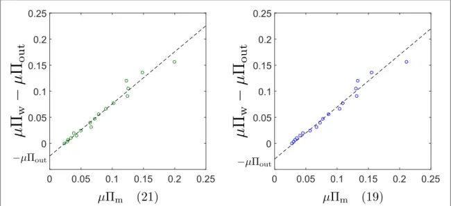
mPout =vs ¥ dzr( )z . (C.3) L

We extractμ Πoutusing a parametric plot of equation(C.2) against equation (21) for all accessible values of z.

We obtain an affine relationship (see figureC1, left). We then measure −μΠoutat the intersect between the affine

fit and the y-axis, and find μΠout=0. 024±0.004 s−1. Note that we could equivalently use equation(19)

(see figureC1, right) but the measurements of Qzz(z) and mz(z) are noisier (figureC2) and the corresponding

estimate ofΠout=0.03±0.005 s−1slightly less reliable.

Appendix D. Sedimentation and active impulse

For the sake of generality, we derive in this appendix the relationship between the bulk pressureΠw(z), as defined

in(8), and momentum and active impulse transfers in the bulk of the active system, in the presence of

translational diffusion. We consider particles evolving with the dynamics h

q

= - +

˙ v ( ) v D ( )

r 0u s ze . D.1

Using Itō calculus, the dynamics of the exact microscopic density field rˆ = å_id(r-ri)is given by[21,37]

r = -ˆ˙ · ˆJ (D.2)

å

r r r q d º -  + L - + -ˆ _{D ˆ Dˆ v ˆ v ( ) ( ) ( )} J 2 s ze u r r , D.3 i i i 0

whereL(r,t)is aδ-correlated Gaussian white noise field of zero mean and unit variance. In a sedimentation profile, the steady state is flux-free leading to a vanishing mean current º á ñ =_J ˆ_{J 0, so that}

Figure B1. Exact angular distribution for 2D ABPs_{(plain lines) and angular distribution for 3D ABPs measured in simulations of} equation(B.1) (symbols).

å

r( )= á q d( - )ñ - ¶r( ) ( ) vs z v cos r r D z , D.4 i i i z 0

where we have introducedrº á ñrˆ and we have used that the system is invariant by translation along ˆx to replace  by∂zand to drop any useless dependence on x. Equation(D.4) simply states that the downward

contribution to the density current due to the sedimentation of the active particles is opposed both by the average upward motion of the particles and by the upward diffusiveflux. For non-interacting ABPs, the first term of the rhs of equation(D.4) can be rewritten as the flux of active impulse [14]. Using Itō calculus, one writes

q d q d q d q d ¶ á - ñ = -á - ñ + Dá - ñ - á - ñ ( ) ˙ ( ) ( ) ( ) ( ) D D r r r r r r r r r

cos cos cos

cos D.5

t i i i i i i i

r i i

so that, in steady state,

q d q d q d

á ( - )ñ = ¶ áD ( - )ñ - ¶ á ˙ ( - )ñ ( )

D D

r r r r z r r

cos i i zz cos cos . D.6

r i i z i r i i Figure C1.mP - Pw m out=vs_òz dzr( )z L

versusμΠm(21) (left) and (19) (right) for experiment with vs/v0=0.29. We use this plot

to measureμΠoutby looking at the intersect between the affine fit y=x+b and the y-axis. We find μΠout=0. 03±0.005 s−1for

(19), and μΠout=0. 024±0.004 s−1for(21).

Figure C2. Blue circles: experimental measurements for mz(left) and Qzz(right) versus z, using equations (17) and(18). Black circles

which is equation(14) of the main text.

We note that the same result can also be obtained, more in line with[14], by considering an underdamped

system and taking the overdamped limit at the end.

Appendix E. Force density exerted by ABPs in a sedimentation profile

In this appendix we detail the computation of the force density exerted by an active system on a confining interface located at height zw:

ò

r

= ¥ ¶

( ) ( ) ( ) ( )

P zz w r V r d .z E.1

zb z w

As before, we compute the dynamics of r ( )r andfind, in the steady state

r˙ ( )r = = -¶0 z zJ( )r , (E.2) where Jzis the mean density current along ˆz, which vanishes in the steady state:

r r m

= = - - ¶ +

( ) ( ) ( ) ( ) ( )

Jz r 0 vs r r z wV v m0 z r. E.3 This allows us to write the mechanical pressure as

ò

ò

m r m = - ¥ + ¥ ( ) ( ) ( ) ( ) P zz w vs dz r v m r d .z E.4 z z z 0 b b

Using Itō calculus, we now compute the dynamics of mz, defined in(17), which yields in the steady-state

å

q d = = -¶ á - ñ -˙ ˙ ( ) ( ) mz 0 z cos z r r D m. E.5 i i i i r z

Together with equation(24), one gets

r m = -¶[ + - - ¶ ] ( ) m v Q D v D m Dm V 2 . E.6 z z zz r s r z r z z w 0

Therefore, the mechanical pressure felt by the boundary is given by

ò

m r m r m = - ¥ ( )+ [ ( )+ ( )]- ( ) ( ) P v z v D Q v v D m r r r r d 2 . E.7 z s z r b zz b s r z b 02 0 b

This expression is valid for anyzbzw. In particular, for zb=zwwe recover equation(26) of the main text.

ORCID iDs

Felix Ginot https://orcid.org/0000-0001-9585-8613 Alexandre Solon https://orcid.org/0000-0002-0222-1347 Julien Tailleur https://orcid.org/0000-0001-6847-3304

Cecile Cottin-Bizonne https://orcid.org/0000-0001-5807-9215

References

[1] Ginot F, Theurkauff I, Levis D, Ybert C, Bocquet L, Berthier L and Cottin-bizonne C 2015 Nonequilibrium equation of state in suspensions of active colloids Phys. Rev. X011004 1_–8

[2] Palacci J, Cottin-Bizonne C, Ybert C and Bocquet L 2010 Sedimentation and effective temperature of active colloidal suspensions Phys. Rev. Lett.105 088304

[3] Enculescu M and Stark H 2011 Active colloidal suspensions exhibit polar order under gravity Phys. Rev. Lett.107 58301

[4] Nash R W, Adhikari R, Tailleur J and Cates M E 2010 Run-and-tumble particles with hydrodynamics: sedimentation, trapping, and upstream swimming Phys. Rev. Lett.104 258101–4

[5] Solon A P, Cates M E and Tailleur J 2015 Active Brownian particles and run-and-tumble particles: a comparative study Eur. Phys. J.: Spec. Top.224 1231–62

[6] Stark H 2016 Swimming in external fields Eur. Phys. J. Spec. Top.225 2369–87

[7] Szamel G 2014 Self-propelled particle in an external potential: existence of an effective temperature Phys. Rev. E90 2704–7

[8] Tailleur J and Cates M E 2009 Sedimentation, trapping, and rectification of dilute bacteria Europhys. Lett.86 60002

[9] Vachier J and Mazza M G 2017 Sedimentation of active particles arXiv:1709.07488

[10] Wolff K, Hahn A M and Stark H 2013 Sedimentation and polar order of active bottom-heavy particles Eur. Phys. J. E36 43

[11] Wagner C G, Hagan M F and Baskaran A 2017 Steady-state distributions of ideal active Brownian particles under confinement and forcing J. Stat. Mech.: Theory Exp.2017 043203

[12] Basu U, Maes C and Netočny` K 2015 How statistical forces depend on the thermodynamics and kinetics of driven media Phys. Rev. Lett.114 250601

[13] Falasco G, Baldovin F, Kroy K and Baiesi M 2016 Mesoscopic virial equation for nonequilibrium statistical mechanics New J. Phys.18 093043

[14] Fily Y, Kafri Y, Solon A P, Tailleur J and Turner A 2018 Mechanical pressure and momentum conservation in dry active matter J. Phys. A: Math. Theor.51 044003

[15] Joyeux M and Bertin E 2016 Pressure of a gas of underdamped active dumbbells Phys. Rev. E93 032605

[16] Junot G, Briand G, Ledesma-Alonso R and Dauchot O 2017 Active versus passive hard disks against a membrane: mechanical pressure and instability Phys. Rev. Lett.119 028002

[17] Mallory S A, Šarić A, Valeriani C and Cacciuto A 2014 Anomalous thermomechanical properties of a self-propelled colloidal fluid Phys. Rev. E89 052303

[18] Razin N, Voituriez R, Elgeti J and Gov N S 2017 Generalized archimedes’ principle in active fluids Phys. Rev. E96 032606

[19] Smallenburg F and Löwen H 2015 Swim pressure on walls with curves and corners Phys. Rev. E92 032304

[20] Solon A P, Fily Y, Baskaran A, Cates M E, Kafri Y, Kardar M and Tailleur J 2015 Pressure is not a state function for generic active fluids Nat. Phys.11 673–8

[21] Solon A P, Stenhammar J, Wittkowski R, Kardar M, Kafri Y, Cates M E and Tailleur J 2015 Pressure and phase equilibria in interacting active Brownian spheres Phys. Rev. Lett.114 1–6

[22] Speck T and Jack R L 2016 Ideal bulk pressure of active Brownian particles Phys. Rev. E93 062605

[23] Takatori S C, Yan W and Brady J F 2014 Swim pressure: stress generation in active matter Phys. Rev. Lett.113 028103

[24] Winkler R G, Wysocki A and Gompper G 2015 Virial pressure in systems of spherical active Brownian particles Soft Matter11 6680–91

[25] Yang X, Manning M L and Marchetti M C 2014 Aggregation and segregation of confined active particles Soft Matter10 6477–84

[26] Barrat J-L, Biben T and Hansen J-P 1992 Barometric equilibrium as a probe of the equation of state of colloidal suspensions J. Phys.-Condens. Matter4 L11–4

[27] Biben T, Hansen J-P and Barrat J-L 1993 Density profiles of concentrated colloidal suspensions in sedimentation equilibrium J. Chem. Phys.98 7330_–44

[28] Buzzaccaro S, Rusconi R and Piazza R 2007 Sticky hard spheres: equation of state, phase diagram, and metastable gels Phys. Rev. Lett.99 098301

[29] Piazza R, Bellini T and Degiorgio V 1993 Equilibrium sedimentation profiles of screened charged colloids: a test of the hard-sphere equation of state Phys. Rev. Lett.71 4267

[30] Piazza R, Buzzaccaro S and Secchi E 2012 The unbearable heaviness of colloids: facts, surprises, and puzzles in sedimentation J. Phys.-Condens. Matter24 284109

[31] Paxton W F, Kistler K C, Olmeda C C, Sen A, St Angelo S K, Cao Y, Mallouk T E, Lammert P E and Crespi V H 2004 Catalytic nanomotors: autonomous movement of striped nanorods J. Am. Chem. Soc.126 13424–31

[32] Ginot F, Theurkauff I, Detcheverry F, Ybert C and Cottin-bizonne C 2018 Aggregation-fragmentation and individual dynamics of active clusters Nat. Commun.9 696

[33] Fily Y and Marchetti M C 2012 Athermal phase separation of self-propelled particles with no alignment Phys. Rev. Lett.108 235702

[34] Yan W and Brady J F 2015 The swim force as a body force Soft Matter11 6234–44

[35] Alhargan F A 1996 A complete method for the computations of Mathieu characteristic numbers of integer orders SIAM Rev.38 239–55

[36] Elgeti J and Gompper G 2015 Run-and-tumble dynamics of self-propelled particles in confinement Europhys. Lett.109 58003–7