HAL Id: hal-00304906
https://hal.archives-ouvertes.fr/hal-00304906
Submitted on 1 Jan 2003HAL is a multi-disciplinary open access archive for the deposit and dissemination of sci-entific research documents, whether they are pub-lished or not. The documents may come from teaching and research institutions in France or abroad, or from public or private research centers.
L’archive ouverte pluridisciplinaire HAL, est destinée au dépôt et à la diffusion de documents scientifiques de niveau recherche, publiés ou non, émanant des établissements d’enseignement et de recherche français ou étrangers, des laboratoires publics ou privés.
Norwegian lakes: relationships with sulphur deposition
and climate indices
P. J. Dillon, B. L. Skjelkvåle, K. M. Somers, K. Tørseth
To cite this version:
P. J. Dillon, B. L. Skjelkvåle, K. M. Somers, K. Tørseth. Coherent responses of sulphate concentration in Norwegian lakes: relationships with sulphur deposition and climate indices. Hydrology and Earth System Sciences Discussions, European Geosciences Union, 2003, 7 (4), pp.596-608. �hal-00304906�
Coherent responses of sulphate concentration in Norwegian
lakes: relationships with sulphur deposition and climate indices
P.J. Dillon
1, B.L. Skjelkvåle
2, K.M. Somers
3and K. Tørseth
41Environmental and Resource Studies, Trent University, Peterborough, Ontario, Canada, K9J 7B8
2Norwegian Institute for Water Research (NIVA), P.O. Box 173, Kjelsaas, N-0411 Oslo, Norway
3Ontario Ministry of the Environment, Dorset Research Centre, P.O. Box 39, Dorset, Ontario, Canada, P0A 1E0
4Norwegian Institute for Air Research (NILU) P.O. Box 100, N-2027 Kjeller, Norway
Email for corresponding author: [email protected]
Abstract
The coherence or synchrony in the trends in SO42 concentration in a set of 100 lakes in Norway that have a long-term chemical record was
evaluated. Using a statistical technique that compares patterns or trends that are not uni-directional, the lakes were grouped into 18 subsets or clusters, each with between 2 and 11 lakes that had similar trends. These temporal trends were strongly correlated with several climate indices, notably the Arctic Oscillation Index (AOI) measured in the autumn, and the annual North Atlantic Oscillation Index (NAOI). Because these clusters of lakes were spatially dispersed, they could not be compared directly with trends in wet S deposition, because S deposition varied substantially between lakes within each cluster. However, the average trend in SO42 concentration was evaluated in each of 10 regions
of Norway that were defined previously on the basis of pollution load, meteorological variables and biogeography. Although these regions did not match the statistically-selected clusters of lakes with equal trends very closely, there were similar, strong correlations between climate indices (the AOI and NAOI) and the 10 average SO42 trends, although there were even stronger relationships with average wet S
deposition in the regions. When subsets of lakes with coherent SO42 trends were selected from within each of the 10 regions, both wet S
deposition and the climate indices were strongly correlated with those SO42 trends. Hence, lakes in Norway respond to changes in wet S
deposition and are influenced by large-scale, i.e. global, climate signals. Future evaluation of recovery of lakes affected by acid deposition must therefore consider the confounding effects of climate and potential climate change.
Keywords: recovery, acid deposition, coherence, sulphate, climate change
Introduction
Since the1980s, enormous scientific effort has been directed towards elucidating whether national and international programmes, implemented to reduce global SO2 emissions and deposition, have been effective in improving chemical and biological conditions in surface waters. Data summarising results of recovery from surface water acidification in Europe and North America due to reductions in S-emission are in Stoddard et al. (1999), Evans et
al.(2001), Stoddard et al. (2003), Jeffries et al. (2003) and
Skjelkvåle et al. (2003).
Although reductions in S deposition in both Europe and North America have led to some recovery of aquatic systems, including decreased SO42 concentrations in many lakes, recovery in many places has been substantially less than initially anticipated, particularly when lake pH and/or acid
neutralising capacity (ANC) are considered. Several factors may contribute to delay or counteract the expected response in surface waters. These include: (1) re-oxidation of reduced S (Dillon and LaZerte, 1992; Schindler et al., 1996; Dillon and Evans, 2001), desorption of previously adsorbed SO42 (Alewell, 2001; Cosby et al., 1986), or mineralisation and oxidation of organically bound S from the catchment (Mitchell et al., 2001); (2) reductions in lake- or stream water base cation (BC) concentrations as a result of either reduced atmospheric BC deposition (Hedin et al., 1987; Gimeno et
al., 2001) or decreased BC leaching from the exchange pool
in the soil (Stoddard et al., 1999); (3) increases in NO3 concentrations in stream- and lake waters due to increase in N-deposition or increased N-leaching (Wright et al., 2001); (4) increases in DOC which may contribute to natural organic acidity of the surface waters and potentially offset
recovery (Ek and Korsman, 2001; Stoddard et al., 2003). Superimposed on any long-term changes that might have occurred in the chemistry of the soils, precipitation and surface waters as a result of decreasing SO2 emissions is the influence of natural year-to-year and between-season variations and cycles in climate parameters, particularly temperature and precipitation. For example, temperature and soil moisture influence mineralisation/decomposition processes, thus affecting cycling of S, N, C and other elements in lakes and catchments. These fluctuations induce variability in surface water chemistry and thus obscure the detection of trends that might be expected as a result of reductions in anthropogenically-related acidic deposition.
The intra- and inter-annual fluctuations in weather are further complicated by the effects of longer-term weather patterns i.e. climate and climate change. Climate as an external factor that has a controlling influence on the behaviour of lake and catchment biogeochemistry has long been recognized (Magnuson et al., 1997). In recent years, several studies of the temporal coherence of lakes, i.e., the degree to which lakes within a given region behave similarly through time, (Magnuson et al., 1990; Soranno et al., 1999), have demonstrated that, for lakes within certain regions, climate often has a greater influence on the physical, chemical and biological properties of the lakes than other external factors, in-lake processes, catchment characteristics, landscape position, etc. In addition, experimental manipulations at the ecosystem scale, e.g. the RAIN and CLIMEX projects (Wright and Jenkins, 2001), have shown clearly that climate is a confounding factor in recovery from acidification. In these studies, increased mineralisation during periods of warmer temperature resulted in increased NO3 leaching.
However, few have addressed the impact of known large-scale climatic patterns or events on surface waters. This may partly be due to lack of long-term, high quality data series necessary for such analysis. Recently, Monteith et al. (2000) related acidification episodes in rivers on the Norwegian west coast to frequency and intensity of sea-salt-episodes and the North Atlantic Oscillation index (NAOI). High positive index values were associated with large amounts of sea-salt deposition, high salt concentrations in the rivers (Cl and Na+) and mobilisation of potentially toxic H+ and aluminium. Strong correlations were found between the NAOI, sea-salt deposition and river data, pointing at the importance of North Atlantic climate variability on acidification. Evans et al. (2001) linked fluctuations in marine ion (Cl, Na+, Mg2+) concentrations to the NAO; an inverse relationship between concentrations of non-marine SO42 and Cl at five lake sites in Great Britain suggested that soil retention and release of SO42 also may be a
sea-salt related process, that would have repercussions for the detection of long term trends in lake recovery. In North America, Dillon et al. (1997) and Dillon and Evans (2001) reported a connection between SO42 redox reactions and El Niño Southern Oscillation (ENSO) episodes; elevated stream SO42- concentrations and export rates in south-central Ontario occurred in the autumn of years with prolonged severe drought and this drought occurred in the years following strong El Niño events, i.e. when the SOI (the Southern Oscillation Index which is used as a measure of the strength of the El Niños), was strongly negative. A climatic link between precipitation patterns in the Great Lakes basin and the two extreme phases of the SOI, i.e. El Niño and La Nica, was established by Shabbar et al. (1997) who reported a distinct pattern of negative precipitation anomalies in the region during the first winter following the onset of El Niño events.
In this paper, the temporal coherence in SO42 concentration has been examined in a set of 100 lakes located in Norway that have experienced significant reductions in SO42 deposition over the past two decades. SO42 has been chosen as a simple indicator of the lakes response to acid deposition. The relationship has been evaluated between patterns in SO42 concentration in the lakes and several large-scale climate indices, including the NAOI, the SOI and the Arctic Oscillation Index (AOI). The AOI has been included because the lakes investigated here are situated at northern latitudes which are influenced by Arctic air masses. The purpose was to evaluate the importance of variations in these climate indices as well as long-term changes in S deposition as factors controlling changes in SO42- concentration in lakes.
Study area
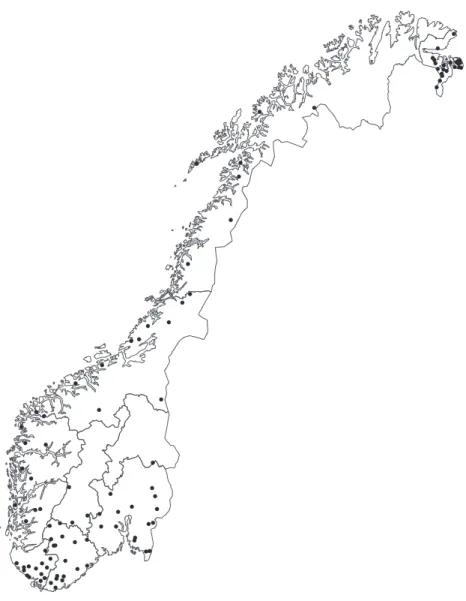
The data used in this work are from the Norwegian national monitoring programme on long-range transboundary air pollution (Skjelkvåle et al., 2001). In the Norwegian monitoring programme (Skjelkvåle et al., 2001), Norway has been divided into 10 regions (Fig. 1) based on empirical knowledge of pollution load (S and N deposition), meteorological variables and biogeography, with each of the ten regions having different water chemistry characteristics (Table 1). All of the regions lakes are acid-sensitive, headwater lakes on granitic or gneissic bedrock without any local pollution sources. All have low ionic strength water containing low base cation and alkalinity concentrations, and SO42 concentrations above background levels (typically 510 µeqL1) found in remote areas with little or no anthropogenic S deposition. The 100 lakes are situated throughout the country, although rather more are in the southern regions.
Fig. 1. Location of the 100 study lakes and the 10 pre-defined regions.
Methods
(I) SAMPLING METHODS
Precipitation samples (bulk) were collected daily or weekly at 30 sites (Fig. 2) and analysed for major solutes at the Norwegian Institute for Air Research (NILU) by standard methods (Skjelkvåle et al., 2001). Concentrations of gases and aerosols were also measured, but are not included in this analysis. The deposition data were averaged for all stations within each of the 10 regions to obtain an average regional value for wet S deposition.
Lake water samples from the subset of the 1000-lake survey of 1986 (Henriksen et al., 1989) were collected annually at the outlet of the lakes after the autumn circulation period. Samples were analysed at the Norwegian Institute of Water Research (NIVA) by standard methods (Skjelkvåle
and Henriksen, 1995). Only lakes with 14 years or more of data were used in this analysis.
Non-marine fractions of SO42 and base cations in lake water were calculated on the assumption that all Cl in lakes is of marine origin (sea-salt) and is accompanied by other ions in the same proportions as in seawater. Thus, the non-marine fraction was equivalent to measured SO42 0.103*Cl-, with parameters expressed on an equivalent basis.
(II) CLIMATE INDICES
Although the effects of climate and climate change on lake or stream chemistry most likely result from changes in precipitation, temperature, radiation, wind speed, etc. on biogeochemical processes in lakes and their catchments, climate indices rather than individual climate parameters
! ( !( ! ( ! ( ! ( ! ( ! ( ! ( ! ( ! ( ! ( ! ( ! ( ! ( ! ( ! ( ! ( ! ( ! ( ! (!( ! ( ! ( !( ! ( ! ( ! ( ! ( ! ( ! ( ! ( ! ( ! ( ! ( ! ( ! ( ! ( !( ! ( ! ( ! ( ! ( ! ( ! ( ! ( ! ( ! ( ! ( ! ( ! ( ! ( ! ( ! ( ! ( ! ( ! ( ! ( ! (!( ! ( ! ( ! ( ! ( ! ( ! ( ! ( ! ( ! ( ! ( ! ( ! ( ! ( ! ( ! ( ! ( ! ( ! ( ! ( !( ! ( ! ( ! ( ! ( ! ( ! ( ! ( !( ! ( ! ( ! ( ! ( ! ( ! ( ! ( ! ( ! ( ! (!!(( ! (
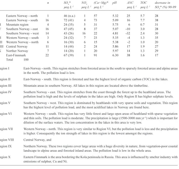
Table 1. Chemical characteristics of lakes in the 10 regions. Mean water chemistry data are for all samples collected from 1990-1999
(one sample for each lake per year, sampled after autumn circulation in the lake). n indicates the number of lakes in each region. For SO42- , number in brackets is the coefficient of variation (%). % decrease in SO42- is based on linear regression. * denotes non-marine fraction.
n SO4* NO3 (Ca+Mg)* pH ANC TOC decrease in
µeq L1 µeq L1 µeq L1 µeq L1 µeq L1 SO
4* (%) 90-99
I Eastern Norway - north 1 46 (n.a.) 1 57 5.32 25 5.7 28 II Eastern Norway - south 16 72 (41) 4 73 5.09 16 7.7 38 III Mountain region 4 24 (35) 5 31 5.75 6 0.7 31 IV Southern Norway - east 16 47 (45) 8 37 5.07 -10 3.0 28 V Southern Norway - west 14 43 (26) 16 22 4.81 -32 2.4 30 VI Western Norway - south 3 24 (32) 7 23 5.35 -4 1.3 35 VII Western Norway - north 6 16 (30) 6 15 5.38 -2 1.0 20 VIII Central Norway 11 14 (44) 2 24 5.86 17 1.9 27 IX Norther Norway 7 14 (20) 1 20 5.97 14 1.3 29
X East-Finnmark 22 67 (39) 1 91 6.30 38 1.6 17
Total 100
Region I East-Norway - north. This region stretches from forested areas in the south to sparsely forested areas and alpine areas in the north. The pollution load is low.
Region II East-Norway - south. This region is forested and has the highest level of organic carbon (TOC) in the lakes. Region III Mountain areas in southern Norway. All lakes in this region are located above the timberline.
Region IV Southern Norway - east. This region stretches from the coast through the forest up to the heathland areas. The pollution load is high and the levels of sulphate in the lakes are high. Only Region II has higher sulphate levels. Region V Southern Norway - west. This region is dominated by heathlands with very sparse soils and vegetation. This region
has the highest level of pollution load, and the most acidified lakes in Norway are found here.
Region VI Western Norway - south. This region has very little forest and large open areas of heathland with sparse vegetation and thin soils. The pollution load is moderate. The precipitation is large (1500-3000 mm yr1) which is important for dilution of the surface waters. The ion concentration in the lakes in this area is very low.
Region VII Western Norway - north. This region is very similar to Region VI, but the pollution load is less and the precipitation is higher. Consequently the ion strength of lakes in this region is the lowest amongst the regions.
Region VIII Central Norway, and
Region IX Northern Norway. These two regions cover large areas with a huge diversity in nature, from vegetation-poor coastal landscape to alpine areas and forested inland areas. The pollution load is low in the whole area.
Region X Eastern Finnmark is the area bordering the Kola peninsula in Russia. This area is influenced by smelter industry with emissions of sulphur, Cu and Ni.
were used in this study. This was done in the absence of any
a priori knowledge of which of the many climate parameters
control these processes, and no complete record of many of them is available all over the country.
Indices describing the North Atlantic Oscillation (NAO), the El Niño Southern Oscillation (ENSO), and the Arctic Oscillation (AO) were used in the statistical analyses to determine if these global-scale phenomena were related to observed changes in the chemistry of the study lakes. The Southern Oscillation Index (SOI) is a standardised measure
of the concurrent differences in atmospheric pressure across the South Pacific Ocean. The occurrence of El Niño is indicated by a negative SOI value for several consecutive months (NOAA, http://www.cpc.noaa.gov/data/indices/soi). The North Atlantic Oscillation Index (NAOI) is a comparable index related to conditions over the Atlantic Ocean, and is calculated using sea level atmospheric pressure differences between Iceland and Gibraltar or the Azores. Similarly, the Arctic Oscillation Index (AOI) relates to Arctic air masses and pressure differentials across that
Fig. 2. Location of the 30 deposition monitoring stations. Wet S deposition (g S m-2 yr1) isopleths are shown.
region. In addition to the annual values for these indices (the sum of the reported monthly values), annual data lagged by one and two years were used because earlier evidence indicated that droughts induced by the El Niño followed the onset of negative SOIs by half a year or more. In addition, seasonal values of the indices were used (each three-month period, with the summer and autumn seasons being those from the previous year), and a seven-month period from September to March, as this window best captured the majority of El Niño events. In this way, each climate phenomenon was used to create eight summary indices.
(III) STATISTICAL METHODS
To evaluate of the effects of S deposition and of climate indices on lake SO42 concentrations, the lakes were grouped in two ways. Firstly, lakes were grouped by the pre-defined ten regions and standardised (z-scored) concentrations were used for each lake in the region to obtain a standardised trend or pattern for that region. These, in turn, were used by region to evaluate relationships with wet S deposition and climate indices. Secondly, coherence analysis was used to select subsets of lakes with statistically similar patterns in SO42 concentration from the complete 100-lake set. In this case, the relationships between standardised concentrations
" " " " " " """ " " " " " " " " " " " " " " " " " " " "" 0.8 0.6 0.2 0.1 0.2
in each of these subsets were evaluated with climate indices only. Finally, coherent or synchronous subsets of lakes were selected from each of the pre-defined ten regions (if there was more than one such subset) for similar analysis, using both deposition and climate indices.
Although Pearson product-moment correlations have been used to evaluate temporal coherence among lakes by comparing time series for all-possible pairs of lakes (Magnuson et al., 1990), temporal coherence in SO42 concentrations between lakes was estimated using the intraclass correlation from a repeated-measures (or randomised block) analysis of variance (ANOVA; Donner, 1986; Somers et al., 1996). The ANOVA was a two-way model without replication, with year as one factor incorporating the repeated-measures nature of the data, and the pair of lakes as the second factor. The two-way interaction term in the ANOVA represents variation between lakes over years (i.e. interaction plus error given no replication). Here, lake is a blocking factor (i.e., this variation is factored out) such that differences in the overall means for each lake are partitioned from the year-to-year variation and ignored. Since this blocking does not control differences in variances that are often correlated with the mean value, the variances for each time series were standardised to unity. The standardisation ensures that the intraclass and Pearson correlations provide the same values, being analogous to using z-scored time series in either approach but with slightly different degrees of freedom (Cronbach and Gleser, 1953). Both the Pearson and intraclass correlations measure the parallel or synchronous nature of the two time series. But, relative to the Pearson correlation, the intraclass correlation is a more general type of correlation that is not restricted to pair-wise comparisons, is better suited when the variables are responses (i.e. measured with error), and it can accommodate missing data.
As in Magnuson et al. (1990), individual correlations summarise temporal coherence among pairs of lakes. Here, time series for 100 lake basins result in 4950 correlations among all-possible pairs of lakes. Evaluating each of these correlations for significance presents a variety of statistical problems (Magnuson et al., 1990); alternatively, an overall test of the entire matrix of between-lake correlations (Brien
et al., 1984) can be used to determine: (1) if the matrix of
between-lake correlations is homogeneous (i.e. all pair-wise correlations are equal and hence, all of the time series are synchronous); and (2) if the average between-lake correlation differs significantly from zero. When, as expected, the full matrix of correlations failed the test of homogeneity (i.e. all of the time series were not synchronous), Rusak et al. (1999) was followed and Briens test used as an exploratory tool to identify homogeneous
subsets of lakes by sequentially examining groups of lakes, an approach akin to cluster analysis.
Subsequently, multiple regression determined which summary climate indices best predicted the SO42 time series. For each climate index, simple correlation and multiple regression identified the seasonal and annual (including lagged data, i.e. annual data offset by one and two years) summaries that best explained the variance in the SO42 patterns (P< 0.10). Because the various seasonal summaries are inter-correlated to varying degrees (i.e. redundant or multi-collinear; Rencher and Pun, 1987), the resultant r, F and P values (and associated partial correlation statistics) were used to identify the best subsets of predictors for each of the SO42 patterns. In the final assessment, the best predictors for each of the climate indices were included in forward- and backwards- selection stepwise multiple regressions to determine which indices accounted for the greatest amount of the between-year variation in multi-lake SO42 concentrations. Again, among-predictor redundancies were minimised to reduce problems with multi-collinearity in the multiple regressions.
Results and discussion
(I) LAKE GROUPINGS
Firstly, the intraclass correlation coefficients (in a 100 × 100 correlation matrix) and Briens test of equal correlations evaluated whether all 100 lakes had coherent or synchronous trends in SO42 concentration. This test indicated that the correlations were not all equivalent, i.e. that the trends were not the same in all lakes, a result that was expected because of the wide range of wet S deposition and measured lake SO42 concentrations found across the country, and because of the large differences in the extent which S deposition has changed between regions of Norway. For example, the wet S deposition has dropped by more than 50% in the southern regions (II-VII in Fig. 1), while the change was much less in the northern portion of the country. In addition, lake chemistry is influenced by the geological setting, and, to a lesser extent, by biological factors. Hence, lake chemistry changes are likely to be non-uniform spatially.
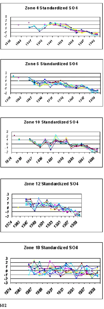
Lakes were then grouped into subsets by picking the mostly strongly correlated pair and adding additional lakes one by one until the next addition resulted in a non-coherent subset. This was done without replacement, i.e. each lake was added to only one group. In this way, the 100 lakes were grouped into 18 subsets of lakes (called clusters in the subsequent discussion), each with a statistically similar trend or pattern in SO42 concentration over time. Five of the 18 clusters are shown in Fig. 3. The degree of similarity
Fig. 3. Standardised SO42- concentration (z-scored, i.e. expressed as the value minus the mean for that series divided by the standard deviation) in lakes in 5 of the 18 clusters that had synchronous or similar patterns. Each line represents data for an individual lake. Cluster 18 includes lakes in the northern-most part of the country, and indicates that long-term trends in lake SO42- are much less here.
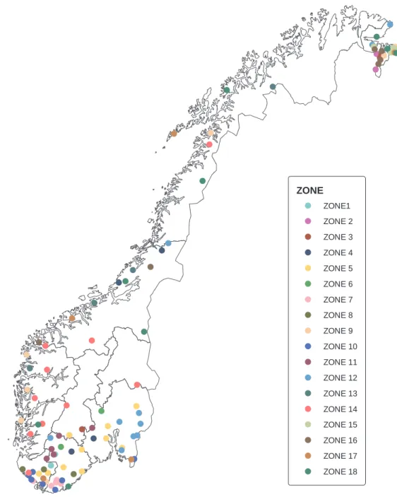
between lakes trends within a cluster clearly varies from one cluster to another; nevertheless, each cluster represents a subset of lakes with statistically similar trends. The z-scored SO42 concentrations for each synchronous cluster or subset of lakes were averaged for each year to produce 18 summary time series, one for each subset of lakes. Based on these summary trends, the lake SO42 concentrations declined in many of the clusters over the course of this study. This was particularly apparent in the southern regions, while changes in the northern areas were much less pronounced. The lake subsets or clusters selected using the statistical method are shown in Fig. 4, along with the ten pre-defined regions. It is clear that the 18 subsets defining clusters of similar trends do not each fall within defined regions; rather, each cluster overlaps with several regions. Conversely, each pre-defined region had several subsets or clusters included, i.e. had lakes with different trends in SO42 concentration.
The alternative scheme evaluated for grouping lakes was the use of the ten regions of Norway that were pre-defined by physiography, meteorology, etc. The advantage of this eco-region approach is that SO42 deposition data are available for one or more stations assigned to each region, and average values for the appropriate parameters can be calculated by region for use in the subsequent analyses. The disadvantage of using this grouping methodology is that the trends or patterns within each region are not necessarily coherent, as evidenced by the statistical analysis producing more (18) lake groups than the number of regions (10), and by the groups of lakes with common trends in no case falling within single regions. On the other hand, the coherence analysis method results in lake groups that each include only those lakes that have similar trends; that is, are recovering or changing at the same rate, making it possible to define each subset or cluster by a single trend line. However, these groupings are not spatially separated or discrete, making it more difficult to assign S deposition measurements or meteorological information to these statistically-defined clusters.
For these reasons, in a third grouping strategy, coherent subsets of lakes within each of the 10 pre-defined regions were defined by carrying out Briens test on lakes that were first grouped into the 10 regional subsets (Fig. 1). In this way, each region had a small number of coherent subsets, although cases such as region one with only two lakes in total cannot be evaluated in this way.
In the subsequent model development, trends in lake SO42 were used in 18 clusters, 10 pre-defined regions, and in coherent subsets of the 10 regions with similar trends.
(II) RELATIONSHIPS WITH CLIMATE INDICES AND WET S DEPOSITION
The factors affecting the average trends in SO42 concentration in lakes grouped into the 18 clusters or subsets of lakes with synchronous trends in SO42 concentration were evaluated first. These clusters, each of which represents a group of lakes with similar SO42 concentration trends,
included between 2 and 11 lakes. When the trends in SO42 concentration were correlated with the climate indices, in 11 of 18 cases statistically significant relationships (p < 0.05) resulted, plus an additional two cases with significance levels between 0.05 and 0.1. The best models, based on stepwise multiple regression analysis where those climate index parameters with significant correlations with lake SO42 were included as possible independent variables, are shown in Table 2. In seven cases, the best model employed the Arctic Oscillation Index (AOI), while three used the North Atlantic Oscillation Index (NAOI), one used both the AOI and the NAOI and two used the Southern Oscillation Index (SOI). Fig. 4. Location of lakes within each of 18 coherent subsets or clusters of lakes with similar SO42- concentration.
!! ! !!! ! ! ! ! ! ! ! ! ! ! ! ! ! ! ! ! ! ! ! !!!!! ! ! ! ! ! ! ! ! ! ! ! ! !! ! ! ! ! ! ! ! ! ! ! ! ! ! ! ! !! ! ! ! ! ! ! ! ! ! ! ! ! ! ! ! ! !!! ! ! !! ! ! ! ! ! ! ! ! ! ! ! ! ! ! ! ! ZONE ! ZONE1 ! ZONE 2 ! ZONE 3 ! ZONE 4 ! ZONE 5 ! ZONE 6 ! ZONE 7 ! ZONE 8 ! ZONE 9 ! ZONE 10 ! ZONE 11 ! ZONE 12 ! ZONE 13 ! ZONE 14 ! ZONE 15 ! ZONE 16 ! ZONE 17 ! ZONE 18
Three of the five clusters with no significant model had the majority of their lakes in the northern part of the country, where there has been relatively little change in either S deposition or lake SO42 concentration. In most instances of significant relationships, seasonal indices rather than annual indices were chosen. In every case where the AOI was selected, the autumn value was chosen, while, in the case of the NAOI, either the spring or annual values were adopted.
The climate indices explained between 25 and 50% of the variability in lake SO42 in the 13 regions with significant relationships. Previously, Monteith et al. (2000) have reported that the NAOI was related to lake chemistry in Norway through its apparent influence on sea-salt episodes, particularly in coastal regions. High positive values of the NAOI generally cause strong westerly winds, frontal precipitation and higher temperatures, which are consistent with positive correlations with lake SO42 concentration. The data presented here provide the first indication that the Arctic Oscillation is also an important climate parameter with respect to lake chemistry, although the mechanism through
which it influences chemistry is unclear. Unlike North America (Dillon et al., 1997; Dillon and Evans, 2001), the SOI was the least important index for Norwegian lakes, a result that is not surprising given that the SOI relates to meteorological conditions in the Pacific Ocean.
While it would be useful to compare the strength of the relationships between trends in S deposition and trends in SO42 concentration in lakes in each cluster with the relationships based on climate indices, it was not possible to assign unique wet S deposition values to each cluster. This is a result of the fact that amalgamation of lakes into subsets with synchronous trends in SO42 concentration yielded subsets that were somewhat scattered spatially.
To evaluate the relative role of changes in S deposition and climate indices, the average standardised trends in lake chemistry measured in each of the 10 pre-defined regions were used. The relationships with climate indices alone were first evaluated using the standardised average lake SO42 trend for all lakes in each region ; the best models based on stepwise multiple regression are shown in Table 3. When this was done, it was found that there were significant
Table 2. Relationships (based on stepwise regression analysis) between long-term trend in z-scored SO4 2-concentration in the 18 clusters or subsets of lakes each consisting of lakes with similar trends and various climate indices. The data record is 14 years in each case. n is the number of lakes in each cluster. For region 4, the model includes 2 independent parameters, while all other models include only 1 parameter, likely because the climate index parameters are strongly correlated with each other.
Cluster n model r2 intercept coefficient P
1 2 AOI (fall) 0.27 0.023 0.37 0.05
2 2 no model
3 3 AOI (fall) 0.31 0.012 0.42 0.037
4 5 NAOI (annlag0) 0.58 0.023
and AOI (fall) 0.64 0.150 0.42 0.008
5 10 AOI (fall) 0.32 0.116 0.38 0.035 6 2 AOI (fall) 0.37 0.081 0.40 0.022 7 5 AOI (fall) 0.46 0.702 0.21 0.007 8 3 SOI (winter) 0.24 0.139 0.12 0.074 9 7 NAOI (annlag1) 0.26 0.075 0.06 0.063 10 7 SOI (winter) 0.39 0.259 0.14 0.017 11 5 no model 12 11 AOI (fall) 0.48 0.059 0.47 0.005 13 4 NAOI (annlag0) 0.40 0.144 0.07 0.015 14 10 no model 15 4 AOI (fall) 0.31 0.023 0.36 0.037 16 6 no model 17 5 NAO (spring) 0.30 0.166 0.16 0.042 18 9 no model
fall = average for Sept-Nov; winter = average for Dec-Feb; spring = average for Mar-May; summer = average for Jun-Aug; annlag0 = annual average for same year; annlag1 = average value for preceding year; annlag2 = annual average 2 years prior
relationships for seven of the 10 regions, the exceptions being region 10 (Fig. 1), the northern-most region where there was very little measured change in lake SO42, and regions 5 and 6 on the south-west coast of the country. There is a considerable number of lakes in the latter two regions, and the coherence analysis discussed previously demonstrated that these lakes grouped into a relatively large number of subsets or clusters (10) with each subset consisting of lakes with similar trends in SO42 concentration. This may reflect different sensitivities to acid deposition of lakes in these regions because of, e.g. variable geology, or more likely may reflect strong gradients in climate-related parameters, e.g. amount of precipitation. This, in turn, could lead to varying response to the climate indices. As was the case with the relationships between climate indices and lake chemistry trends in the 18 clusters (Table 2), the strongest relationships for the 7 regions were with either the AOI (four cases) or the NAOI (two cases) or both (one case). In these region-based models, 30 to 60% of the variability in lake SO42 was explained by these indices, again demonstrating the importance of climate in the trends. In all cases when an AOI parameter was chosen, it was the fall value, while the NAOI parameter selected was either the annual or spring value. The choices of these particular seasonal indices are entirely consistent with the selections made independently for the models describing lake trends by coherent clusters. However, it is somewhat surprising that SO42 in the southern regions (I-IV), although not the southern coastal regions (V-VII), was most strongly correlated with the AOI, while
the northern regions appeared to be influenced most by the NAOI rather than the AOI.
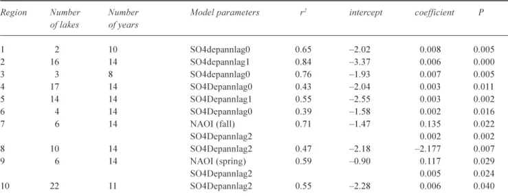
To evaluate the relative importance of both S deposition and the climate indices to the trends in SO42 concentration within each of the 10 regions, the analysis was repeated with both the same climate indices and the average standardised wet S deposition by region as possible independent variables. When this was done (Table 4), the best relationships were with S deposition parameters in most cases, although in two regions (7 and 9), the NAOI was also important. These models explained between 40 and 85% of the variability, significantly more than climate indices alone. However, this approach suffers from the fact that the pre-defined 10 regions do not represent sets of lakes that behave coherently, i.e. have the same trends. They are grouped on the basis of pollution load (S and N deposition), meteorology and biogeography, rather than on the basis of parameters that might be expected to have the most impact on their response to changes in S (and N) deposition, e.g. geology, initial lake chemistry, etc.
To address this, coherence analysis was used to define synchronous subsets within each of the 10 regions rather than by selecting from the entire 100-lake set. The result was that regions with larger numbers of lakes had multiple coherent subsets with similar trends in SO42 concentration, for example, region 5 with 14 lakes had three discrete subsets, while region 10 with 22 lakes had six subsets. In all, 25 coherent subsets were formed from the 10 regions. When we carried out multiple regression analysis, first with
Table 3. Results of stepwise regression analysis of average (z-scored) trend in SO42- concentration of all lakes in each of the pre-defined 10 regions with the various climate indices. Only models that were significant at the p<0.05 level are shown.
Region Number Number Model parameters r2 intercept coefficient P
of lakes of years 1 2 14 AOI (fall) 0.40 0.052 0.40 0.015 2 16 14 AOI (fall) 0.40 0.083 0.43 0.015 3 3 14 AOI (fall) 0.33 0.086 0.42 0.031 4 17 14 AOI (fall) 0.31 0.120 0.32 0.038 5 14 14 no model 6 4 14 no model 7 6 14 NAOI (spring) 0.53 0.212 0.15 0.032 NAOI (fall) 0.17 0.021 8 10 14 NAOI (annlag0) 0.58 0.146 0.05 0.024 AOI (fall) 0.27 0.029 9 6 14 NAOI (spring) 0.33 0.110 0.14 0.030 10 22 14 no model
fall = average for Sept-Nov; winter = average for Dec-Feb; spring = average for Mar-May; summer = average for Jun-Aug; annlag0 = annual average for same year; annlag1 = average value for preceding year; annlag2 = annual average 2 years prior
climate indices alone, 19 of the 25 coherent subsets had significant models, explaining between 21 and 86% of the variability in SO42- trend. In Table 5, the relative frequency of selection of each climate index chosen for any model is shown. Eleven of the 19 models were based on, or included, the AOI, while four utilised the NAOI and four the SOI. As in the earlier analyses, the fall AOI was the most frequently selected parameter. When we included S deposition as well as the climate indices as potential independent variables, 24 of the 25 subsets produced significant models, with between 38 and 99% of the variance in SO42 trend explained. The frequency of variable selection is summarized in Table 5; again, S deposition was most commonly selected, but the AOI, NAOI and on occasion, the SOI were also correlated significantly in many regions. In all instances where the AOI was important, the subsets of lakes were located in regions 8 to 10, i.e. in the northern half of the country. Conversely, the models for subsets of lakes in the southern part of Norway, where deposition changes have been greatest, relied much more heavily on S deposition than the climate indices.
In future, it would be useful to try to determine how the climate indices affect lake chemistry, i.e. which meteorological variables are influenced or correlated with the indices, particularly the AOI and the NAOI. It has been pointed out that the NAOI governs inter-annual variability in precipitation over northern Europe (Monteith et al., 2000), and since precipitation amount determines runoff and lake water replenishment rate, it is not surprising that the NAO
Table 4. Results of stepwise regression analysis of average (z-scored) trend in SO42- concentration of all lakes in each of the pre-defined 10 regions with the various climate indices and wet S deposition in that region (standardised average of all deposition stations within that region). Only models that were significant at the p<0.05 level are shown.
Region Number Number Model parameters r2 intercept coefficient P
of lakes of years 1 2 10 SO4depannlag0 0.65 2.02 0.008 0.005 2 16 14 SO4depannlag1 0.84 3.37 0.006 0.000 3 3 8 SO4depannlag0 0.76 1.93 0.007 0.005 4 17 14 SO4Depannlag0 0.43 2.04 0.003 0.011 5 14 14 SO4Depannlag1 0.55 2.55 0.003 0.002 6 4 14 SO4Depannlag0 0.39 1.58 0.002 0.016 7 6 14 NAOI (fall) 0.71 1.47 0.135 0.022 SO4Depannlag2 0.002 0.002 8 10 14 SO4Depannlag2 0.47 2.18 2.177 0.007 9 6 14 NAOI (spring) 0.59 0.90 0.117 0.029 SO4Depannlag2 0.005 0.024 10 22 11 SO4Depannlag2 0.55 2.28 0.006 0.040
fall = average for Sept-Nov; winter = average for Dec-Feb; spring = average for Mar-May; summer = average for Jun-Aug; annlag0 = annual average for same year; annlag1 = average value for preceding year; annlag2 = annual average 2 years prior
Table 5. Frequency of selection of variables in the multiple
regression analysis based on coherent subsets of lakes from within each of the 10 regions. There were a total of 25 such subsets. Frequency A refers to models that used only climate indices, while Frequency B refers to models that could choose both wet S deposition parameters and climate indices. Most models selected only one parameter from each general group, e.g. only one AOI parameter, because the method used takes colinearity into account.
Parameter Frequency A Frequency B
AOI (fall) 10 4
AOI (winter) 1 3
AOI (annual) 1 2
AOI (annual lag1) 1
-AOI (spring) - 1
NAOI (spring) 2 1
NAOI (fall) 1 1
NAOI (annual) 2 3
NAOI (annual lag1)
SOI (winter) 3 2
SOI (annual) 2 2
S dep (annual) 8
S dep (annual lag1) 8 S dep (annual lag 2) 6
is important. The mechanism whereby the AO affects lake chemistry is less clear but, as the AOI was even more strongly related to trends in SO42 than the NAOI, it is important to evaluate this further.
Summary
The decline in wet S deposition in Norway, which varies in a gradient from south to north, has altered lake chemistry, particularly in the south. Lake SO42 has decreased wherever there has been an appreciable decrease in S deposition. Using coherence analysis, lakes were grouped according to those with similar trend or pattern. A set of 100 lakes with long-term data, located throughout the country, were grouped into 18 separate subsets or clusters, each consisting of lakes with statistically similar SO42 concentration trends. These clusters differed somewhat from the 10 regions defined on the basis of ecosystem characteristics alone, in that the clusters generally included lakes in two or more regions, and in a few cases, spanned a large portion of the country. When correlations between the trends in SO42 concentration within the clusters and three climate indices (the North Atlantic Oscillation, Arctic Oscillation and Southern Oscillation indices) were investigated, in almost all cases, significant models that explained 2550% of the variance in SO42 resulted. The AOI, especially the autumn value, and the annual NAOI were the indices most often and most strongly correlated with the SO42 trends. The relative importance of S deposition could not be assessed because the clusters defining coherent subsets of lakes were, in some cases, spread over relatively large portions of the country. This precluded assigning S deposition values or trends to each cluster.
When average SO42 concentration trends in lake water in the 10 pre-defined regions were related to climate indices, the AOI and NAOI were again dominant, producing strong relationships in almost every region. When average wet S deposition in each region was also included as an independent variable, it provided stronger individual models, but a combination of S deposition and the NAOI sometimes gave the best relationship. When coherent or synchronous subsets of lakes within each region were evaluated, S deposition and climate indices together always yielded the best models.
These results prove that lakes in Norway respond to both changes in S deposition and to large-scale, i.e. global, climate signals, and future evaluation of recovery of lakes affected by acid deposition must consider the confounding effects of climate and potential climate change. This implies that catchment processes such as redox cycles and mineralisation, that are influenced by climate variables including precipitation and temperature, which in turn, affect hydrology, are certain to be important in assessing recovery of aquatic systems.
Acknowledgments
Thanks are due to J. Findeis for assistance with the data analysis, to H. Evans for providing a literature review and to the Ontario Ministry of the Environment for logistical support for this work. This work was funded by grants from Ontario Power Generation Inc. and the Natural Sciences and Engineering Research Council of Canada to PJD. This work was conducted as part of a collaborative research programme between Trent University and the Commission of European Communities RECOVER: 2010 project (EKVI-CT-1999-00018).
References
Alewell, C., 2001. Predicting reversibility of acidification: The European sulfur story. Water Air Soil Pollut., 130, 12711276. Brien, C.J., Venables, W.N., James, A.T. and Mayo, O., 1984. An analysis of correlation matrices: equal correlations. Biometrika,
71, 545554.
Cosby, B.J., Hornberger, G.M., Wright, R.F. and Galloway, J.N., 1986. Modelling the effects of acid deposition: control of long-term sulfate dynamics by soil sulfate adsorption. Water Resour.
Res., 22, 12831291.
Cronbach, L.J. and Gleser, G.C., 1953. Assessing similarity between profiles. Psychol. Bull., 50, 456473.
Dillon, P.J. and LaZerte, B.D., 1992. Response of the Plastic Lake catchment, Ontario to reduced sulphur deposition. Environ.
Pollut., 77, 211217.
Dillon, P.J. and Evans, H.E., 2001. Long-term changes in the chemistry of a soft-water lake under changing acidic deposition rates and climate fluctuations. Verh. Internat. Verein. Limnol.,
27, 26152619.
Dillon, P.J., Molot, L.A. and Futter, M., 1997. The effect of El-Niño-related drought on the recovery of acidified lakes. Environ.
Monitor. Assess., 46, 105111.
Donner, A., 1986. A review of inference procedures for the intraclass correlation coefficient in the one-way random effects model. Int. Statist. Rev., 54, 6782.
Ek, A.S. and Korsman, T., 2001. A paleolimnological assessment of the effects of post-1970 reduction of sulfur deposition in Sweden. Can. J. Fisheries Aquat. Sci., 58, 16921700. Evans, C.D., Cullen, J., Alewell, C., Kopácek, J., Marchetto, A.,
Moldan, F., Prechtel, A., Rogora, M., Veselý, J. and Wright, R.F., 2001. Recovery from acidification in European surface waters. Hydrol. Earth Syst. Sci., 5, 283298.
Gimeno, L., Marin, E., Del Teso, T. and Bourhim, S., 2001. How effective has been the reduction of SO2 emissions of the effect of acid rain on ecosystems? Sci. Total Environ., 275, 6370. Hedin, L.O., Likens, G.E. and Bormann, F.H., 1987. Decrease in
precipitation acidity resulting from decreased SO4 2-concentration. Nature, 325, 244246.
Henriksen, A., Lien, L., Rosseland, B.O., Traaen, T.S. and Sevaldrud, I., 1989. Lake acidification in Norway - present and predicted fish status. Ambio, 18, 314321.
Jeffries, D.S., Clair, T.A., Couture, S., Dillon, P.J., Dupont, J., Keller, W., McNicol, D.K., Turner, M.A. and Weeber, R., 2003. Assessing the recovery of lakes in Southeastern Canada from the effects of acid deposition. Ambio, 32, 176182.
Magnuson, J.J., Benson, B.J. and Kratz, T.K., 1990. Temporal coherence in the limnology of a suite of lakes in Wisconsin, U.S.A. Freshwater Biol., 23, 145159.
Magnuson, J.J., Webster, K.E., Assel, R.A., Bowser, C.J., Dillon, P.J., Eaton, J.G., Evans, H.E., Fee, E.J., Hall, R.I., Mortsch, L.R., Schindler, D.W. and Quinn, F.H., 1997. Potential effects of climate changes on aquatic systems: Laurentian Great Lakes and Precambrian shield region. Hydrol. Process., 11, 825871. Mitchell, M.J., Mayer, B., Bailey, S.W., Hornbeck, J.W., Alewell, C, Driscoll, C.T. and Likens, G.E., 2001. Use of stable isotope ratios for evaluating sulphur sources and losses at the Hubbard Brook Experimental Forest. Water Air Soil Pollut., 130, 7586. Monteith, D.T., Evans, C.D. and Reynolds, B., 2000. Are temporal variations in the nitrate content of UK upland freshwaters linked to the North Atlantic Oscillation? Hydrol. Process., 14, 1745 1749.
Rencher, A.C. and Pun, F.C., 1987. Inflation of R2 in best subset regression. Technometrics, 22, 4953.
Rusak, J.A., Yan, N.D., Somers, K.M. and McQueen, D.J., 1999. The temporal coherence of zooplankton population abundances in neighboring north-temperate lakes. Amer. Naturalist, 153, 4658.
Schindler, D.W., Bayley, S.E., Parker, B.R., Beaty, K.G., Cruikshank, D.R., Fee, E.J., Schindler, E.U. and Stainton, M.P., 1996. The effects of climatic warming on the properties of boreal lakes and streams at the Experimental Lakes Area, northwestern Ontario. Limnol. Oceanogr., 41, 10041017.
Shabbar, A., Bonsal, B. and Khandekar, M., 1997. Canadian precipitation patterns associated with the Southern Oscillation.
J. Climate, 10, 30163027.
Skjelkvåle, B.L. and Henriksen, A., 1995. Acidification in Norway - status and trends. Surface and ground water. Water Air Soil
Pollut., 85, 629634.
Skjelkvåle, B.L., Tørseth, K., Aas, W. and Andersen, T., 2001. Decrease in acid deposition-recovery in Norwegian surface waters. Water Air Soil Pollut., 130, 14331438.
Skjelkvåle, B.L., Evans, C.D., Larssen, T., Hindar, A. and Raddum, G.G., 2003. Recovery from acidification in European surface waters: A view to the future. Ambio, 32, 170175.
Somers, K.M., Reid, R.A., David, S.M. and Ingram, R., 1996. Are the relative abundances of orconectid crayfish better indicators of water-quality changes than cambarid abundances?
Freshwater Crayfish, 11, 249265.
Soranno, P.A., Webster, K.E., Riera, J.L. Kratz, T.K., Baron, J.S., Bukaveckas, P.A., Kling, G.W., White, D.S., Caine, N., Lathrop, R.C. and Leavitt. P.R., 1999. Variation among lakes within landscapes: Ecological organization along lake chains.
Ecosystems, 2, 395410.
Stoddard, J.L., Jeffries, D S., Lükewille, A., Clair, T.A., Dillon, P.J., Driscoll, C.T., Forsius, M., Johannessen, M., Kahl, J.S., Kellogg, J.H., Kemp, A., Mannio, J., Monteith, D., Murdoch, P.S., Patrick, S., Rebsdorf, A., Skjelkvåle, B.L., Stainton, M.P., Traaen, T.S., van Dam, H., Webster, K.E., Wieting, J. and Wilander, A., 1999. Regional trends in aquatic recovery from acidification in North America and Europe 1980-95. Nature,
401, 575578.
Stoddard, J.L., Kahl, J.S., Deviny, F.A, DeWalle, D.R, Driscoll, C.T., Herlihy, A.T., Kellogg, J.H., Murdoch, P.S. and Webster, K.E., 2003. Responses of Surface Water Chemistry to the Clean
Air Act Amendments of 1990. EPA 620/R-03/001, EPA United
States Environmental Protection Agency, 78 pp.
Wright, R.F. and Jenkins, A., 2001. Climate change as a confounding factor in reversibility of acidification: RAIN and CLIMEX projects. Hydrol. Earth Syst. Sci., 5, 477486. Wright, R.F., Alewell, C., Cullen, J., Evans, C.D., Marchetto, A.,
Moldan, F., Prechtel, A. and Rogora, M., 2001. Trends in nitrogen deposition and leaching in acid-sensitive streams in Europe. Hydrol. Earth Syst. Sci., 5, 299310.