A case study carried out with two different NWP systems

HAL Id: hal-00299361

https://hal.archives-ouvertes.fr/hal-00299361

Submitted on 4 Sep 2006

HAL is a multi-disciplinary open access

archive for the deposit and dissemination of

sci-entific research documents, whether they are

pub-lished or not. The documents may come from

teaching and research institutions in France or

abroad, or from public or private research centers.

L’archive ouverte pluridisciplinaire HAL, est

destinée au dépôt et à la diffusion de documents

scientifiques de niveau recherche, publiés ou non,

émanant des établissements d’enseignement et de

recherche français ou étrangers, des laboratoires

publics ou privés.

A case study carried out with two different NWP

systems

P. Kållberg, A. Montani

To cite this version:

P. Kållberg, A. Montani. A case study carried out with two different NWP systems. Natural Hazards

and Earth System Science, Copernicus Publications on behalf of the European Geosciences Union,

2006, 6 (5), pp.755-760. �hal-00299361�

www.nat-hazards-earth-syst-sci.net/6/755/2006/ © Author(s) 2006. This work is licensed under a Creative Commons License.

and Earth

System Sciences

A case study carried out with two different NWP systems

1_{SMHI, S-601 76 Norrköping, Sweden}

2_{ARPA-SIM, Viale Silvani 6, 40122 Bologna, Italy}

Received: 25 October 2005 – Revised: 16 May 2006 – Accepted: 16 May 2006 – Published: 4 September 2006

Abstract. A model intercomparison between two atmo-spheric models, the non–hydrostatic Lokal Modell (LM) and the hydrostatic HIgh Resolution Limited Area Model (HIRLAM) is carried out for a one-week period, including a case of cyclogeneis leading to heavy precipitation over Northern Italy. The two models, very different in terms of data-assimilation and numerics, provide different results in terms of forecasts of surface fields. Opposite diurnal biases for the two models are found in terms of screen level temper-atures. HIRLAM wind speed forecasts are too strong, while LM precipitation forecasts have larger extremes. The inter-comparison exercise identifies some systematic differences in the weather products generated by the two systems and sheds some light on the biases of the two numerical weather prediction systems.

1 Introduction

Limited area data assimilation and forecast experiments with different numerical weather prediction (NWP) systems us-ing identical resolutions and applied to the same observa-tional database are of considerable interest. In particular can the differences between the resulting analyses and forecasts identify systematic errors (“biases") in the systems. Such an experiment has been carried out with two participating sys-tems jointly at ARPA–SIM in Bologna and at SMHI in Nor-rköping, as a part of the research project Carpe Diem sup-ported by the European Commission under the 5th Frame-work Programme (official web site: http://carpediem.ub.es/ home/). At ARPA–SIM a version of the DWD Lokal Modell (hereafter, LM) was used (Steppeler et al., 2002), while ver-sion 6.1 of the HIgh Resolution Limited Area Model (here-Correspondence to: P. Kållberg

(per.kallberg@smhi.se)

after, HIRLAM) system was used at SMHI (Undén et al., 2002).

A synoptic situation from November 1999 with a north-westerly flow across the Alps leading to an intense cycloge-nesis over the Gulf of Genoa was selected. This event pro-duced copious precipitation over northern Italy and was of special interest for the Carpe Diem project. November 1999 was also within the Mesoscale Alpine Programme (hereafter, MAP; Bougeault et al., 2001) with an enhanced observa-tional coverage over continental Europe.

For this case study, LM and HIRLAM were run both se-lecting the same integration domain, which covered conti-nental Europe, and using the same horizontal resolution of

0.1◦on a rotated latitude/longitude grid. In addition to this,

the same sets of observations and lateral boundary conditions were taken from the ECMWF observational archive and op-erational analyses so as to drive the limited area integrations. For both models, data assimilation cycles and sets of fore-casts (starting at 00:00 UTC and 12:00 UTC and ranging up to 48 h) were run from 3 to 9 November 1999, thus covering the MAP IOPs (Intensive Observation Periods) 14 and 15. Here, the attention is focused on the sub-period between 5 and 8 November 1999 (MAP IOP 15), when the cyclogene-sis took place.

2 Description of the NWP systems

As previously described, LM and HIRLAM present a num-ber of common features, as summarised in Table 1. Despite these similarities, it is immediately worth pointing out that basic differences exist between the two forecast systems: for example, the LM forecast model is non-hydrostatic (that is, vertical velocities are a prognostic variable of the model) and the data assimilation is performed with a nudging technique (Davies and Turner, 1977). On the other hand, HIRLAM is hydrostatic (vertical velocities are diagnosed from other

756 P. Kållberg and A. Montani: Case study with different NWP systems

Table 1. Main common features in LM and HIRLAM integrations.

horizontal resolution 0.1◦ grid point_x 224 grid point_y 202

vertical resolution 40 model levels vertical coordinate hybrid pressure–based initial conditions ECMWF analyses boundary conditions 3-hourly ECMWF analyses

model variables) and the data assimilation is done with 3D-Var, a three-dimensional variational technique (Gustafsson et al., 2001; Lindskog et al., 2001). The two models also have different orographies and a different distribution of the ver-tical levels (although the total number of levels is 40 in both NWP systems), this having a possible impact on the genera-tion of post-processed surface variables like mean-sea-level pressure (as shown in Sect. 3). These, and the other model differences existing in terms of numerical and physical ap-proximations, act in such a way that the same observations and lateral boundary conditions, once ingested in the mod-els, may provide rather different forecasts. In the next two subsections, the two limited–area models are described in greater detail, so as to emphasise the main features of each forecasting system.

2.1 The ARPA-SIM system

The COnsortium for Small-scale MOdelling (COSMO) is a joint development formed in October 1998 and has as members the national meteorological services of Germany, Greece, Poland and Switzerland (for further details, the official COSMO web-site can be found at: http://www. cosmo-model.org). In addition to this, the regional weather service ARPA-SIM (Italy) and the military service AWGeo-phys (Germany) within the member states are participating in the project. The general goal of COSMO is to develop, improve and maintain the non-hydrostatic limited-area atmo-spheric model LM (Steppeler et al., 2003), used for both op-erational and research applications by the COSMO members. The model equations of LM are solved numerically using the Eulerian finite difference method. By defaults, second-order centred finite difference operators for both horizontal and vertical differencing are used, although other options are present. A hybrid sigma-type (with respect to base-state pressure) vertical coordinate is used. The time integration method used in LM is a leapfrog scheme (horizontally ex-plicit, vertically implicit), including the extensions proposed by Skamarock and Klemp (1992). Lateral boundary condi-tions are provided using the relaxation technique of Davies and Turner (1977). The parameterisation of physical pro-cesses include grid-scale cloud and precipitation, subgrib-scale clouds, moist convection, radiation, vertical diffusion,

surface layer and soil processes. The data-assimilation is done using a nudging-based assimilation scheme, where the model prognostic variables are relaxed towards direct obser-vations within a predetermined time window (Davies and Turner, 1977). Currently, only conventional observations are used, namely from TEMP, PILOT, AIRCRAFT, SYNOP, SHIP and DRIBU. For these experiments, LM was used with 40 vertical hybrid coordinate levels. The ARPA-SIM experi-ment will be identified as “ARP” from now on.

2.2 The SMHI system

HIRLAM (Undén et al., 2002) is a joint development by sev-eral European countries of an operational data-assimilation and short-range forecast system for their National Weather

Services. The numerical approximation of HIRLAM

in-cludes both a gridpoint version and a spectral version, with either Eulerian or semi–Lagrangian time integration. Lat-eral boundary conditions are prescribed with the boundary relaxation technique (Davies and Turner, 1977). The physi-cal parameterisation includes turbulence closure with turbu-lent kinetic energy as a prediction parameter (Cuxart et al., 2000), long and short-wave radiation with cloud interaction (Savijarvi, 1989), and stratiform and convective precipita-tion according to the STRACO scheme (Sass et al, 1999). The semi-Lagrangian gridpoint configuration of HIRLAM was used with 40 vertical hybrid coordinate levels. The data assimilation was done with a three-dimensional variational technique, 3D-Var (Gustafsson et al., 2001; Lindskog et al., 2001), using so called “conventional" observations from the MAP period as collected at ECMWF. The 3D-Var assimi-lation was run with six hour cycling and the “FGAT" (First Guess at Appropriate Times) approach. Five different exper-iments were made with the SMHI system, but in this paper we will only cover the control experiment, from here called “CDC”, which is directly comparable with ARP. A crucial component of the variational analysis process is the assump-tion made on the errors of the background forecast, in this case a 6-h forecast. The original structure functions used in CDC were originally developed for the SMHI operations which were run with considerably lower horizontal tion. A revised set, recently determined for higher resolu-tion operaresolu-tions, was used in an experiment which is not fur-ther described here; suffice it here to note that it did produce somewhat finer structures in the analyses and forecasts.

3 Comparisons with own analyses

Although the forecast experiments were “technically” run up to a range of 48 h, here the attention is focused over a shorter prediction range (namely, 24 h). It is thought that longer-term limited area forecasts over a small domain (like the one used in these experiments) are primarily just a down-scaling of the ECMWF forecasts and not very interesting in

-1 -6 -4 0 0 -2 -4 7 4 3 -3 4 6 -7 -5 9 -9 6 3 -8 3 8 7 -1 4 8 -15 10 -4 11 10 0 2 8 2 2 -2 5 -2 0 2 -25 -10 -7 -4 -2 -1 1 2 4 7 10

and the +24h for

1000 1000 1010 1010 1020 1020 1020 1020 1030 1030 1032 1021 1029 1009 1018 1024 1012 994 1031 1032 1030 1028 1024 1021 1018 1021 1016 ___and the +24h forecast difference to it. ___Pmsl analysis

Sun 7 Nov 1999 00Z +00h - Sat 06 Nov 1999 00Z +24h

valid Sun 7 Nov 1999 00Z ARPASIM 11 km.

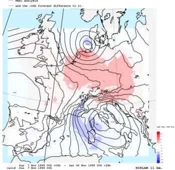
Fig. 1. ARP analysis valid at 00:00 UTC, 7 November in terms of

mean-sea-level pressure (in hPa, solid contours), together with the forecast error in the 24-h forecast valid at this time (in hPa, shaded areas: red positive, blue negative).

our kind of study. Therefore, the most interesting 24-h fore-casts for the Genoa cyclone development were those starting at 00:00 UTC and 12:00 UTC on 6 November. Figures 1 and 2 show the mean sea level pressure analyses at 00:00 UTC on 7 November (contours), together with the deviation (er-ror) of the corresponding 24-h forecast (shaded). The anal-ysed mean sea level pressure is extrapolated from the sur-face pressure at the model’s orography, and we can note that this extrapolation introduces some noise in the ARP analyses over high terrain, e.g. the Alps and the Pyrenees. The CDC analyses exhibit some kinks in the boundary relaxation zone. Disregarding these minor cosmetic differences, the two anal-yses are very similar.

Both systems capture the development well, but we can note that the ARP forecast errors are noisier and with some-what larger amplitudes. Both systems predict too high sures over central Europe north of the Alps and too low pres-sures near and west from Corsica/Sardinia, i.e. the cyclone is slightly too far west.

4 Comparisons with observations

Rather than making too many comparisons with own analy-ses, we will compare the analyses and the 24-h forecasts from ARP and CDC directly with the synoptic observations. The ARP analyses and forecasts at/from 12:00 UTC, 5 November were not available for this verification. In Table 2, the

-1 -1 -1 0 -1 0 -3 2 2 1 -1 -2 -1 -1 1 -4 1 1 2 -1 0 0 3 -1 -2 -4 2 -4 2 5 4 2 1 4 4 -1 2 2 1 1 -25 -10 -7 -4 -2 -1 1 2 4 7 10

and the +24h for

1000 1000 1010 1010 1020 1020 1028 1008 1024 999 1000 1002 1027 1030 1030 1029 1021 1017 1014 1027 1014 1003

___and the +24h forecast difference to it. ___Pmsl analysis

Sun 7 Nov 1999 00Z +00h - Sat 06 Nov 1999 00Z +24h

valid Sun 7 Nov 1999 00Z HIRLAM 11 km.

Fig. 2. The same as Fig. 1, but for CDC analysis and 24-h forecast.

Table 2. Mean sea level pressure standard deviation (in hPa) of

analyses and 24-h forecasts against SYNOP/SHIP observations in the full area.

initial st. dev. ana st. dev. ana st. dev. fc st. dev. fc

time (ARP) (CDC) (ARP) (CDC)

5 Nov 00Z 1.27 0.81 1.19 1.02 6 Nov 00Z 1.31 0.92 1.74 1.58 6 Nov 12Z 1.18 0.84 1.16 0.99 7 Nov 00Z 1.00 0.73 0.89 0.99 7 Nov 12Z 0.95 0.77 1.14 0.95 Mean 1.14 0.81 1.22 1.11

dard deviation of analyses and 24-h forecasts versus all avail-able SYNOP and SHIP observations of the mean sea level

pressure are summarised. Observations obviously wrong

were removed by a crude filter. A better procedure would certainly have been to verify against only those observations accepted by the analysis procedures themselves, but this in-formation was not available from both experiments. Again we can note somewhat lower scores for ARP, possibly re-lated to the post-processing of the mean sea level pressure.

Tables 3 and 4 show the mean biases and standard devi-ations of the screen level temperatures. It is interesting to note the opposing biases in the two analyses; ARP is biased cool at daytime and warm at nighttime, while CDC is warm at daytime and cool at night. Both forecast models chill too much in their 24-h forecasts, CDC considerably more so than ARP. The cooling bias in the HIRLAM model has also been

758 P. Kållberg and A. Montani: Case study with different NWP systems

Table 3. Screen level temperature bias (in◦C) of analyses and 24-h forecasts against SYNOP/SHIP observations in the full area.

initial bias ana bias ana bias fc bias fc time (ARP) (CDC) (ARP) (CDC) 5 Nov 00Z +0.58 −0.10 −0.48 −0.01 6 Nov 00Z +0.18 −0.09 −0.15 −0.48 6 Nov 12Z −0.28 +0.16 −0.06 −0.10 7 Nov 00Z +0.60 −0.05 −0.18 −1.06 7 Nov 12Z −0.43 +0.17 +0.01 −0.47 Mean +0.13 +0.03 −0.17 −0.42

Table 4. Screen level temperature standard deviation (in◦C) of analyses and 24-h forecasts against SYNOP/SHIP observations in the full area.

initial st. dev ana st. dev. ana st. dev. fc st. dev. fc

time (ARP) (CDC) (ARP) (CDC)

5 Nov 00Z 1.49 1.37 1.74 1.91 6 Nov 00Z 1.55 1.46 1.88 1.76 6 Nov 12Z 1.48 1.39 1.70 1.62 7 Nov 00Z 1.49 1.44 1.69 1.76 7 Nov 12Z 1.36 1.32 1.54 1.59 Mean 1.47 1.40 1.71 1.73

noted in the SMHI operational forecasts (L. Häggmark, per-sonal communication). The differences in standard deviation of the screen level temperatures between the two systems are negligible. The two systems exhibit noticeable differences in the 10-m wind speed at sea, as shown in Table 5. The ARP analyses have a strong diurnal variation with too weak wind speed analyses at daytime and too strong at night. The CDC speed analyses are always too strong compared with the SHIP observations (differences larger than 5 m/s are ex-cluded from these comparisons). Both systems produce too strong winds in the 24-h forecasts, CDC however twice as large. The positive bias in the HIRLAM 10-m winds has also been found at SMHI, and is related to the parameterisation of the turbulent momentum flux in the planetary boundary layer (PBL).

5 Precipitation

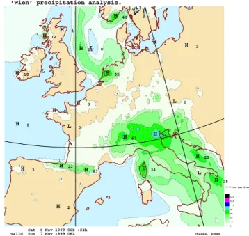
In this section some figures of the predicted 24-h precipi-tation are compared with analyses made from gauge data (Rubel and Rudolf, 2001). The gauge analyses in Fig. 3 are from 06:00 UTC, 6 November to 06:00 UTC, 7 Novem-ber, and so is the accumulated precipitation from CDC in Fig. 4. The ARP precipitation was accumulated only from the 00:00 UTC and 12:00 UTC forecasts, and both are shown

1 1 1 1 1 1 1 1 1 1 1 1 1 1 1 1 1 1 1 1 1 1 1 1 40 H 2 H 25 L 3 H 34 H 25 H 3 H 22 H 23 H 54 H 61 H 0 _{L 0} L 0 H 3 H 3 H 18 L 0 H 35 H 2 H 5 H 21L 0 H 12 H 4 H 40 1 5 10 20 40 70 100 150 ****-hr Tot.Prec

’Wien’ precipitation analysis.

Sat 6 Nov 1999 06Z +24h

valid Sun 7 Nov 1999 06Z Thanks, ECMWF

Fig. 3. Rubel-Rudolf rain gauge analysis of the 24-h

precipita-tion from 06:00 UTC, 6 November to 06:00 UTC, 7 November (in mm/day). 1 1 1 1 1 1 1 1 1 1 1 1 1 1 1 1 1 1 1 1 1 1 1 1 1 1 1 1 11 1 1 1 40 40 40 40 H 8 H 1 H 14 H 8 H 7 L 0 H 0 H 55 H 2 H 27 L 2 H 3 H 66 L 0 H 74 H 22 H 6 H 37 L 1 H 78 H 9 L 0 H 9 H 97 H 50 H 73H 85 H 6 H 11 H 6 H 3 L 0 H 8 H 3 H 20 H 3 H 3 H 16 H 2 H 7 H 1 L 3 H 3 H 19 H 6 H 0 1 5 10 20 40 70 100 150 ****-hr Tot.Prec

Carpe Diem. experiment: cdc

Sat 6 Nov 1999 06Z +24h

valid Sun 7 Nov 1999 06Z Hirlam 6.1 0.1*0.1

Fig. 4. 24-h precipitation accumulation (in mm/day) from forecast

CDC beginning at 06:00 UTC, 6 November.

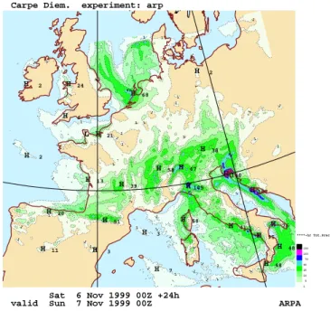
in Figs. 5 and 6, respectively. We note that the ARP forecasts contain more fine-structures and intense precipitation max-ima, as could be expected from a non-hydrostatic model. The hydrostatic CDC produces smoother larger-scale

fea-tures that agree somewhat better with the analyses. The

Table 5. 10-m wind-speed bias (m/s) of analyses and 24-h forecasts

against SHIP observations in the full area.

initial bias ana bias ana st. dev. fc bias fc time (ARP) (CDC) (ARP) (CDC) 5 Nov 00Z +0.36 +0.42 +0.45 +1.04 6 Nov 00Z +0.00 +0.38 +0.59 +0.89 6 Nov 12Z −0.91 +0.40 +0.13 +0.67 7 Nov 00Z +0.26 +0.55 +0.40 +0.77 7 Nov 12Z −0.46 +0.27 +0.44 +0.61 Mean −0.15 +0.40 +0.40 +0.80

Rubel-Rudolf gauge analyses are available on a 0.2 grid, making them still smoother in appearance.

The differences between CDC and ARP rainfall forecasts are due, among other factors, to differences in the model for-mulation and, to a lesser extent, to the small discrepancies in the initial conditions. It is clear that the different PBL pa-rameterisations schemes used in the two limited-area-models have a great impact on the surface fields predicted by the two NWP systems. The different convection schemes used in LM and HIRLAM (and their interaction with orography precip-itation mechanisms) play a major role in the different struc-tures of the predicted precipitation fields. In addition to this, the difficulty in observing and analysing properly the initial humidity fields can be considered another possible source of the forecast differences. Since the forecast model itself is used to assimilate the variables, the two models also make a different use of the same variables to be assimilated, this causing some differences (small but not negligible) in the ini-tial conditions.

6 Conclusions

Two very different NWP systems (data-assimilation and forecast) have been applied to the same synoptic situation with identical horizontal resolution and integration area. The same observations were used, and the same lateral boundary conditions were applied in both experiments. One remain-ing difference, the choice of orography, complicates compar-isons of post-processed variables such as mean sea level pres-sure and prespres-sure level geopotential, and it is recommended, for future experiments, that the same orographies are used. Also, to eliminate post–processing differences, future inter-comparisons should preferably be made directly from the model variables rather than the post-processed products.

The main value of this intercomparison is the identification of biases in some near surface variables, indicating system-atic problems in the parameterisation schemes of both mod-els. 1 1 1 1 1 1 1 1 1 1 1 1 1 1 1 1 1 1 1 1 1 1 1 1 1 1 1 1 1 1 1 1 1 1 1 1 1 1 1 1 1 1 1 1 1 1 1 1 1 1 1 1 1 1 1 1 40 40 40 40 40 40 40 40 H 48 H 7 H 48 H 95 H 76 H 3 H 41 H 11 H 3 H 58 H 51 H 152 H 20 H 105 H 140 H 39 H 67 H 13 H 58 H 38 H 2 H 21 L 0 H 6 H 68 H 2 H 24 H 2 1 5 10 20 40 70 100 150 ****-hr Tot.Prec

Carpe Diem. experiment: arp

Sat 6 Nov 1999 00Z +24h

valid Sun 7 Nov 1999 00Z ARPA

Fig. 5. 24-h precipitation accumulation (in mm/day) from forecast

ARP beginning at 00:00 UTC, 6 November.

1 1 1 1 1 1 1 1 1 1 1 1 1 1 1 1 1 1 1 1 1 1 1 1 1 1 1 1 1 1 1 1 1 1 1 1 1 1 1 1 1 1 1 1 1 40 40 40 40 40 40 40 40 40 40 40 40 40 L 2 H 132 H 72 H 46 H 6 H 9 L 0 H 154 H 38 L 1 H 200 H 12 H 150 H 6 H 1 H 14 H 6 H 6 H 33 H 17 H 5 H 24 1 5 10 20 40 70 100 150 ****-hr Tot.Prec

Carpe Diem. experiment: arp

Sat 6 Nov 1999 12Z +24h

valid Sun 7 Nov 1999 12Z ARPA

Fig. 6. 24-h precipitation accumulation (in mm/day) from forecast

ARP beginning at 12:00 UTC, 6 November.

– The two models have opposite diurnal biases in the

screen level temperatures.

– The HIRLAM screen level temperature forecasts are

760 P. Kållberg and A. Montani: Case study with different NWP systems

– The HIRLAM 10-m wind speed forecasts are too

strong, especially over the sea, possibly due to too large downward momentum fluxes in the PBL parameterisa-tion.

– The LM precipitation forecasts have finer structures

and larger extremes, while the HIRLAM precipitation agrees better (visually) with the gauge analyses. Although this little experiment lasted only one week and in-cluded only one major meteorological event, the exercise identified some systematic differences in the weather prod-ucts generated by the two systems. Further insight may be gained from other (and longer) periods of experimentation, and also from cross-over tests where forecasts are run from each other’s analyses, i.e. ARP forecasts from CDC analyses and vice versa.

It is not trivial to assess the hydrological implications of the model discrepancies. The extent to which atmospheric model differences have either a larger or smaller impact on hydrometeorological forecasting chains, may depend, among other factors, on the size of the river catchment. It is likely that, if the hydrological model is run over a small catchment area, then the discharge forecast differences will be higher due to the faster response to the different rainfall predicted fields. In view of a possible operational implementation of a flood forecasting chain, long experimentation would be needed before drawing firm conclusions. Several months of tests are probably necessary in order to assess benefits and weaknesses of using either one NWP system or another one “to feed” the hydrological model, also for short forecast ranges.

Acknowledgements. The authors are grateful to F. Boccanera,

ARPA–SIM, who performed the ARP runs, and to M. Lindskog, SMHI, for very helpful assistance in using the HIRLAM system. Edited by: L. Ferraris

Reviewed by: two referees

References

Bougeault, P., Binder, P., Buzzi, A., Dirks, R., Houze, R., Kuettner, J., Smith, R. B., Steinacker, R., and Volkert, H.: The MAP Spe-cial Observing Period, Bull. Amer. Meteorol. Soc., 82, 433–462, 2001.

Cuxart, J., Bougeault, P., and Redelsperger, J.-L.: A turbulence scheme allowing for mesoscale and large eddy simulations, Quart. J. Roy. Meteorol. Soc., 126, 1–31, 2000.

Davies, H. C. and Turner, R. E.: Updating prediction models by dynamical relaxation: An examination of the technique, Quart. J. Roy. Meteorol. Soc., 103, 255–245, 1977.

Gustafsson, N., Berre, L., Hörmquist, S., Huang, X.-Y., Lindskog, M., Navascués, B., Mogensen, K. S., and Thorsteinsson, S.: Three-dimensional variational data assimilation for a limited area model. Part I: General formulation and the background error con-straint, Tellus, 53A, 425–446, 2001.

Klemp, J. B. and Wilhelmson, R.: The simulation of three-dimensional convective storm dynamics, J. Atmos. Sci., 35, 1070–1096, 1978.

Lindskog, M., Gustafsson, N., Navascués, B., Mogensen, K. S., Huang, X.-Y., Yang, X., Andræ, U., Berre, L., Thorsteinsson, S., and Rantakokko, J.: Three-dimensional variational data assimi-lation for a limited area model. Part II: Observational handling and assimilation experiments, Tellus, 53A, 447–468, 2001. Rubel, F. and Rudolf, B.: Global daily precipitation estimates

proved over the European Alps, Meteorologische Zeitschrift, 10(5), 407–418, 2001.

Sass, B. H., Nielsen, N. W., Jørgensen, J. U., and Amstrup, B.: The Operational HIRLAM System at DMI, DMI Tech Rep. no 99-21, 1999.

Savijärvi, H.: Fast Radiation Parameterization Schemes for Mesoscale and Short-Range Forecast Models, J. Appl. Meteo-rol., 29, 437–447, 1989.

Skamarock, W. C. and Klemp, J. B.: The stability of time-split nu-merical methods for the hydrostatic and the non-hydrostatic elas-tic equations, Mon. Wea. Rev., 120, 2109–2127, 1992.

Steppeler, J., Doms, G., Schattler, U., Bitzer, H.-W., Gassmann, A., Damrath, U., and Gregoric, G.: Meso-gamma scale forecasts using the non-hydrostatic model LM, Meteorol. Atmos. Phys., 82, 75–96, 2003.

Undén, P., Rontu, L., Jarvinen, H., et al.: HIRLAM-5 Scientific Documentation, SMHI S-601 76 Norrkoping, Sweden, 2002.