HAL Id: hal-01372563
https://hal.archives-ouvertes.fr/hal-01372563
Submitted on 27 Sep 2016
HAL is a multi-disciplinary open access
archive for the deposit and dissemination of
sci-entific research documents, whether they are
pub-lished or not. The documents may come from
teaching and research institutions in France or
abroad, or from public or private research centers.
L’archive ouverte pluridisciplinaire HAL, est
destinée au dépôt et à la diffusion de documents
scientifiques de niveau recherche, publiés ou non,
émanant des établissements d’enseignement et de
recherche français ou étrangers, des laboratoires
publics ou privés.
A Statistical Framework for Conditional Extreme Event
Attribution
Pascal Yiou, Aglaé Jézéquel, Philippe Naveau, Friederike Otto, Robert
Vautard, Mathieu Vrac
To cite this version:
Pascal Yiou, Aglaé Jézéquel, Philippe Naveau, Friederike Otto, Robert Vautard, et al.. A Statistical
Framework for Conditional Extreme Event Attribution. Advances in Statistical Climatology,
Mete-orology and Oceanography, Copernicus Publications, 2017, 3, pp.17-31. �10.5194/ascmo-3-17-2017�.
�hal-01372563�
A Statistical Framework for Conditional Extreme Event Attribution
Pascal Yiou
1, Aglaé Jézéquel
1, Philippe Naveau
1, Frederike E. L. Otto
2, Robert Vautard
1, and
Mathieu Vrac
11Laboratoire des Sciences du Climat et de l’Environnement, UMR 8212 CEA-CNRS-UVSQ, U Paris-Saclay, IPSL, Gif-sur-Yvette, France
2Environmental Change Institute, School of Geography and the Environment, University of Oxford, Oxford, UK Correspondence to:P. Yiou ([email protected])
Abstract. The goal of the attribution of individual events is to estimate whether and to what extent the risk of an extreme climate event evolves when external conditions (e.g. due to anthropogenic forcings) change. Many types of climate extremes are linked to the variability of the large-scale atmospheric circulation. It is hence essential to decipher the roles of atmospheric variability and increasing mean temperature in the change of probabilities of extremes. It is also crucial to define a background state (or counterfactual) to which recent observations are compared. In this paper we present a statistical framework to determine the
5
dynamical (linked to the atmospheric circulation) and thermodynamical (linked to slow forcings) contributions to the risk of extreme climate event. We discuss the creation of two states (or “worlds”) in which risk change is determined. We illustrate this methodology on a record precipitation event that hit southern UK in January 2014. The paper argues that it is possible to obtain qualitative results from reanalysis model simulation data for such an event.
1 Introduction
10
Many extreme events that occur on a local scale are specific to large-scale atmospheric patterns (e.g., rainfall, windstorms, heatwaves in Europe, and phases of the North Atlantic Oscillation). If such links have been identified, changes in the probability of local extremes can be due to changes in the properties of the atmospheric circulation or changes in the link between the local variable and the circulation (which can remain unchanged). The first cause is sometimes qualified as “dynamic” because it refers to the motion of the atmosphere. The second cause is qualified as “thermodynamic” (or “non dynamic”), because it
15
implicitly assumes that the local variable is related to the local change of atmospheric physical properties (e.g., temperature, water content) in the absence of flow changes (Trenberth et al., 2015).
The extreme event attribution (EEA) consists in estimating if and how the probability of an extreme event depends on the climate forcings (National Academies of Sciences Engineering and Medicine, 2016). One of the outcomes is the assessment whether anthropogenic forcings alter such probability. This type of study has been used for estimates of liability for extreme
20
events that caused damages (Allen, 2003).
The first scientific challenge of EEA is to define two worlds to be compared. The EEA studies speak of a factual world when all climate forcings (natural and anthropogenic) forcings are considered (Stott et al., 2004). This is presumably a world that “is”, and in which an event is observed with probability p1. The counterfactual world contains only natural forcings, and is a world
that “might have been”. In such a world, the same extreme event would occur with probability p0. Defining a counterfactual world is a difficult task because it is a possible but non observed state of climate. Then, some studies define the fraction of attributable risk (FAR), which is the relative change of probability between the two worlds FAR ≡ (p1− p0)/p1= 1 − p0/p1 (Stott et al., 2004). Other combinations of the p0 and p1 probabilities also provide pieces of valuable information (Hannart et al., 2016).
5
An alternative approach can be proposed, as in van Haren et al. (2013): a “new” world in which we live, like the recent decades, and an “old” world in which our ancestors lived, like the beginning of the 20th century. We implicitly assume that those two worlds are different (at least from the enviromnental point of view). The main feature of this approach is that it can be based on observed data. It is difficult to decipher the natural and anthropogenic forcings between “old” and “new”. Therefore such a data-based approach can only provide qualitative information on EEA, from implicit hypotheses in the forcing changes,
10
like “greenhouse gas forcing” is larger in the “new” world than in the “old” world.
A second challenge is to determine the dynamical and thermodynamical contributions to the change of probabilities. The goal is to estimate the contribution of atmospheric variability in climate change, and to determine how the properties of a local climate variable change if the atmospheric circulation is fixed. This is advocated by a “storyline” approach to describe a class of extreme events, by understanding the general synoptic conditions leading to the extremes (Trenberth et al., 2015; Shepherd,
15
2016). The storyline approach is designed to decompose the role of climate change in the dynamical and thermodynamical contributions. From a statistical point of view, this motivates the term “conditional attribution”: we investigate how the proba-bility of a local extreme event that depends on a large-scale atmospheric circulation is affected by global climate change or the properties of the circulation itself. If we focus on precipitation extremes, the issue is to evaluate changes in atmospheric flows leading to high precipitation (the dynamical contribution) and changes in precipitation rates given a favourable atmospheric
20
flow (the conditional thermodynamical contribution) (Trenberth et al., 2015).
Recently, Schaller et al. (2016) showed that the change in winter circulation explained about one third of the simulated changes in the large January rain amounts, by using a simple index characterizing stormy weather in the UK. In a recent study, Vautard et al. (2016) generalized this approach for estimating dynamical contribution of changes for a class of extremes characterized by a threshold exceedance. That method used flow analogues combined in the factual and counterfactual worlds,
25
tracking changes in probabilities of exceedance for all flows encountered in each world. Here a direct Bayesian approach is proposed, which also highlights the role of a specific flow type in the event class change.
For illustration purposes we focus on the heavy precipitation event that occurred in Europe in January 2014, which has been investigated by many authors (Huntingford et al., 2014; Matthews et al., 2014; Christidis and Stott, 2015; Schaller et al., 2016). This event was a record precipitation in southern UK, Brittany and Normandy (France). It caused over 570 million euros
30
insured losses in the UK (Schaller et al., 2016).
Section 2 explains the notation and methodology that is developed in the paper. Section 3 details the datasets that are used to define two worlds. Section 4 gives the results of the analyses from the two datasets. We compare the Bayesian analyses with the two sets of worlds (factual and counterfactual vs. new and old). The results are discussed in Section 5 and conclusions appear in Section 6.
2 Methodology
2.1 Notations and rationale
We assume that a climate variable R (e.g. temperature, precipitation) and atmospheric circulation C (e.g. SLP, geopotential height at 500hPa) are observed in a universe that contains two distinct worlds, W0and W1. Here, R is a real variable and C
5
is a two dimensional field. For the first universe, we use Detection and Attribution notations (e.g. Stott et al., 2016; National Academies of Sciences Engineering and Medicine, 2016) to qualify W1 as “factual” and W0 as “counterfactual”. In the second universe W1 is “new” and W0 is “old”. The W1 worlds are close to the one in which we live, either in terms of anthropogenic/natural climate forcings or in terms of temporal proximity (e.g. the last decades). The W0worlds contain only natural climate forcings, or temporal remoteness (e.g. beginning of 20th century (1900–1950) vs. recent decades (1950–2016)).
10
We define an extreme event (in either worlds and universes) when a reference threshold Rref for R has been reached or exceeded. A “class of events” includes the ensemble of weather types for which the threshold can be reached. In the paper, we assume that such an extreme event is reached during a spell of atmospheric circulation Crefin the world W1.
The goal of extreme event attribution is to determine how the probability of an extreme event differs between W1and W0. Achieving this goal is trivial if a rare event occurs in one of the worlds and is impossible in the other. In practice, this does
15
not happen for most extreme events that have occurred in the past decades, because there are often historical examples of such events (e.g. most European winter storms, European heatwaves). Thus, we assume that a given extreme or rare climate event has a probability of occurrence p1in W1, and p0in W0.
The probabilities p1and p0are defined by:
pi= Pr(R(i)> Rref), (1)
20
where R(i)is the climate variable R in the Wiworld, and i ∈ {0, 1}.
For obvious pragmatic reasons, we can assume that p1> 0, because we want to study an event that was observed in the real world. In addition, p1can be fixed to a quantile of the probability distribution of R in W1(e.g. p1= 0.01 for a one in a century event in the factual world). This defines a class of events (here: high values of R). Therefore there is no uncertainty in the determination of p1. The uncertainty lies on an estimate of Rreffrom W1data (if 1/p1is larger than the size of W1), and in p0.
25
We want to estimate the ratio p0/p1, determine its uncertainty and investigate how it is controlled by physical factors. Those physical factors include changes in the probability distribution of the circulation C between W1and W0and the changes in the probability distribution of R if C is similar in W1and W0. We introduce the notion of vicinity of circulation trajectories, or the neighborhood V of an observed circulation Cref. The trajectory neighborhood will be defined in two ways: from the distance to a known weather regime (section 2.3.1), which is computed independently of the event itself, or from the distance
30
2.2 Bayesian formulation
The probabilities pithat the climate variable R(i)exceeds a threshold Rrefand that the atmospheric circulation C(i)lives in the neighborhood of Cref(i.e., C(i)∈ V(Cref)) in the world Wi(i ∈ {0, 1}) are related by the Bayes formula:
pi≡ Pr(R(i)> Rref) = Pr(R(i)> Rref|C(i)∈ V(Cref))
5
× Pr(C(i)∈ V(Cref))
/ Pr(C(i)∈ V(Cref)|R(i)> Rref). (2)
The three terms of the right hand side of Eq. (2) can be computed from data in the two worlds Wi.
The ratio ρ = p0/p1is then decomposed into three terms that can yield physical interpretations. The first one is the “ther-modynamical" change between the two worlds for a given circulation:
10
ρthe≡Pr(R(0)> Rref|C(0)∈ V(Cref)) Pr(R(1)> Rref|C(1)∈ V(Cref))
. (3)
In this term, the circulation is fixed to one that is close to Cref, and changes of the probability of R are due to causes like an increased temperature (increasing the water availability in the atmosphere (Peixoto and Oort, 1992)). If the Crefpattern is prone to high precipitation, this conditional term allows a closer focus on the tail of the distribution of R.
The second term accounts for changes in the patterns of the atmospheric circulation and is hence called “circulation”:
15
ρcirc≡Pr(C(0)∈ V(Cref)) Pr(C(1)∈ V(Cref))
. (4)
It is important to note that Crefis the same in the numerator and denominator. The circulation term measures the change of likelihood of observing circulation sequences that look like Cref.
The third term is a reciprocity condition for the circulation trajectory C: ρrec≡Pr(C(1)∈ V(Cref)|R(1)> Rref)
Pr(C(0)∈ V(Cref)|R(0)> Rref)
. (5)
20
This term determines the extent to which the circulation Crefis necessary when R > Rref. For a fixed Rrefprecipitation rate, it evaluates how likely a circulation like Crefis. This reciprocity term allows one to connect the risk based approach of EEA, based on the study of ρ alone (Shepherd, 2016) to the “storyline approach” (Trenberth et al., 2015; National Academies of Sciences Engineering and Medicine, 2016) that involves the processes that drive the extreme precipitation.
The product ρdyn≡ ρcirc× ρrecdefines the dynamical contribution of the atmospheric change to the precipitation extreme
25
conditional to a fixed thermodynamics. The reciprocity term explores the extent to which the circulation is close to the observed one when the cumulated precipitation is high. This multiplicative decomposition of probabilities can be compared with the “additive” decomposition of Shepherd (2016, Eq. (1)), who also introduces a non-dynamical term.
Sampling uncertainties on those three ratios can be determined by bootstraping over the elements of Wi. The estimation procedure is the following:
1. Determine p1(for example a century return period) and an empirical Rref(for example from W1). 2. Determine the neighborhood of Cref(for example from the monthly frequency of a weather regime).
3. Determine ρthe, ρcirc, ρrecand their probability distribution for the two worlds (for example by bootstrapping over W i). We then assess whether ρthe, ρcircand ρrecare significantly different from 1 by comparing their probability distributions.
5
We will illustrate this approach on the high precipitation event of the winter 2013/2014 in southern UK. 2.3 Circulation neighborhood
In this section, we propose two ways of defining the neighborhood of the circulation Cref. This has an impact on the computa-tion of the thermodynamical and dynamical terms of the decomposicomputa-tion of ρ.
2.3.1 Proximity based on weather regimes
10
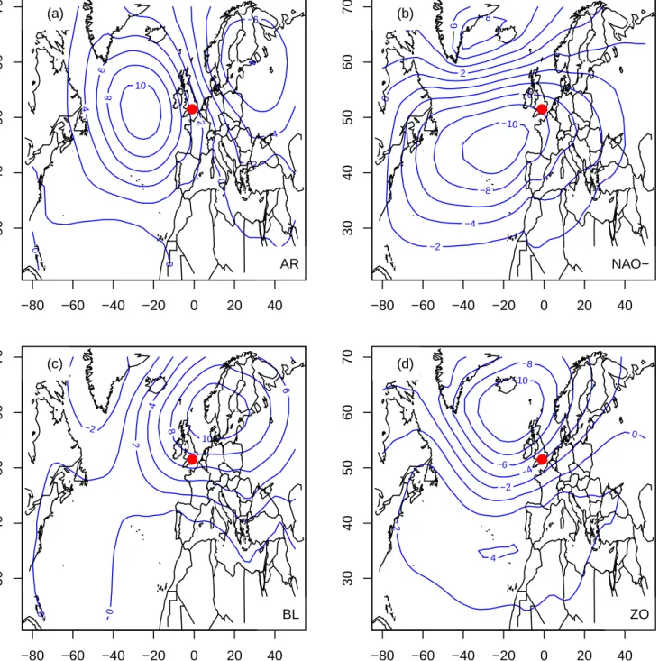
High winter precipitation in Europe is generally associated with zonal atmospheric circulation. The circulation around the North Atlantic can be described by four weather regimes, which are quasi-stationary states of the atmosphere (Vautard et al., 1988; Kimoto and Ghil, 1993; Michelangeli et al., 1995). Those weather regimes are obtained by a k-means classification of anomalies of the winter sea-level pressure (SLP) daily field from the NCEP reanalysis (Michelangeli et al., 1995; Yiou et al., 2008). The weather regime centroids are shown in Figure 1.
15
The frequencies of the weather regimes are computed for each winter (December, January, February). Very wet winters in the UK or North Western France occur when the frequencies of Zonal or NAO− weather regimes are high (> 75%). The average frequency of the zonal weather regime is close to 25% and the frequency reached 81% in January 2014. The two other weather regimes (Scandinavian blocking and Atlantic Ridge) do not lead to very high precipitation rates in southern UK. The zonal weather regime favors warm temperatures in Europe, while NAO− favors cold temperatures (Yiou and Nogaj, 2004;
20
Cattiaux et al., 2010).
The atmospheric trajectories can then be tracked by daily sequences of weather regimes. We summarize the information of a trajectory over a whole winter season (or a single winter month) by the frequencies of the four weather regimes. Hence, if Crefwas mainly zonal (as was the winter of 2013/2014), we will say that the circulation C is in the neighborhood of Cref (C ∈ V(Cref)) if the frequency of the zonal weather regime exceeds 75%. This definition obviously oversimplifies the notion of
25
circulation neighborhood, but it gives an intuitive and qualitative understanding of the atmospheric circulation. This approach is also taken for consistency with the study of Schaller et al. (2016).
2.3.2 Proximity based on analogues of circulation
The computation of weather regimes provides an intuitive and physical interpretation of the atmospheric circulation patterns. But the atmospheric flow trajectories that are considered are, by construction, just closer to one of the weather regime centroids
30
−6 −4 −2 0 0 0 2 4 6 8 10 −80 −60 −40 −20 0 20 40 30 40 50 60 70 ● AR (a) −10 −8 −6 −4 −2 0 0 2 4 6 8 −80 −60 −40 −20 0 20 40 30 40 50 60 70 ● NAO− (b) −2 0 0 2 4 6 8 10 −80 −60 −40 −20 0 20 40 30 40 50 60 70 ● BL (c) −10 −8 −6 −4 −2 0 2 4 −80 −60 −40 −20 0 20 40 30 40 50 60 70 ● ZO (d)
Figure 1. Four winter (DJF) weather regimes of the North Atlantic, computed from the SLP anomalies (in hPa) of NCEP reanalysis. (a): Atlantic Ridge; (b): NAO−; (c): Scandinavian Blocking; (d): Zonal. The red circle indicate the region where high precipitation was observed.
of weather regimes. Hence we also explore the atmospheric circulation with so-called analogues, which exploit explicitly a distance to a reference observed circulation pattern sequence.
If C(d) is the SLP during some day d, the analogues of C are the days dkin a different year, for which the Euclidean distance d(C(d), C(dk)) is minimized. This defines analogues of circulation, based on SLP. Here we consider the North Atlantic sector
5
(80W–50E; 25N–70N) to compute the distance between two SLP patterns, as in (Yiou et al., 2013). We take the K = 20 best analogues of circulation for each day.
A justification to use analogues of circulation to describe the January 2014 atmospheric circulation comes from the fact that the SLP had a rather unusual pattern, which did not have all the characteristics of the zonal weather regime shown in Fig. 1. We illustrate this in Fig. 2 with the mean of analogues from W0and W1. The mean SLP yields a rather steep gradient over UK
10
and France. This steep SLP gradient is better reproduced in the analogue mean than in the ZO weather regime.
A heuristic way to define the neighborhood of the trajectory Cref (e.g., a sequence of C(d) with days in January 2014) is to compute the mean (over the days) of a quantile of the distances of K best analogues. This value can be modulated by a “safety” factor to ensure that there are enough trajectories around Cref to construct statistics. This defines a neighboring “tube” around Crefin the SLP phase space. This threshold is computed from the analogues of Crefin January 2014 for the NCEP reanalyses
15
(1950–2016, excluding January 2014) and gives a value of ≈ 12 hPa for a median quantile of the K = 20 best daily analogues and a “safety” factor of 1.5.
In addition to a definition of proximity, we use the dates of the best SLP analogues simulate reconstructions of climate variables. Here we focus on precipitation R. From a statistical perspective, the analogue precipitations are random “replicates” of the precipitation at the day conditioned by the atmospheric circulation. This allows a determination of the probability
20
distributions of precipitation (R) variability conditioned to the atmospheric circulation C.
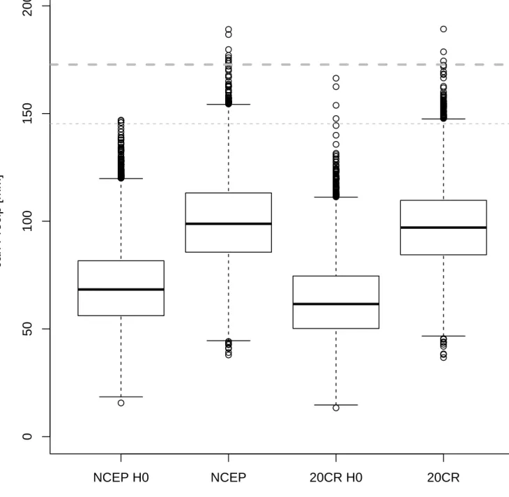
Analogues of C and R provide a natural way of computing the probabilities in Eq. (2). We compute this estimate from the reanalysis datasets (W0= 20CR and W1= NCEP). By contrast, we test the null hypothesis H0 that circulation does not play a role in the high precipitation rate by computing the probability distribution of cumulated precipitation in January when random days are drawn in W0= 20CR and W1= NCEP. Figure 3 emphasizes the rejection of this null hypothesis because
25
the distribution of analogue cumulated precipitation probabilities are significantly higher than for random days.
The ρ term is estimated by random resampling of daily R values in January and computing a monthly average. The proba-bility distribution simulations of R in January 2014 for circulation analogues in W0= 20CR and W1= NCEP are shown in Figure 3. For comparison purposes, mean precipitation taken from random days in the two worlds are also shown, to emphasize the role of the circulation in the high precipitation event in January. This figure shows a slight increase of the probability of
30
having high precipitation in the “new” world with respect to the “old” world. The uncertainty on ρ can be estimated from those boxplots.
The thermodynamical term is estimated from probabilities of R for analogues of Cref in W1 and W0. The first step is to compute analogues of Cref (the circulation in January 2014) in the two reanalysis datasets. For each day d of January 2014, we draw random circulation analogues in W1and W0, and keep the sequence of their dates. Then we compute the sum of the
35
985 990 995 1000 1005 1005 1010 1015 1020 1020 1025 1025 −80 −60 −40 −20 0 20 40 30 40 50 60 70 ● SLP Jan 2014 (a) 990 995 1000 1005 1005 1010 1015 1020 1020 1020 1020 1025 −80 −60 −40 −20 0 20 40 30 40 50 60 70 ● ZO weather regime (b) 990 995 1000 1000 1005 1010 1015 1020 1020 1025 1025 −80 −60 −40 −20 0 20 40 30 40 50 60 70 ● 20CR SLP analogues (c) 990 995 1000 1005 1005 1010 1015 1015 1020 1020 1020 1025 −80 −60 −40 −20 0 20 40 30 40 50 60 70 ● NCEP SLP analogues (d)
Figure 2. Mean SLP of January 2014 (in hPa) for (a): NCEP reanalysis (b): ZO weather regime computed from NCEP (Figure 1d); (c): Mean of analogues in 20CR; (d): Mean of analogues in NCEP. The red circle indicate the region where high precipitation was observed.
● ● ● ● ● ● ● ● ● ● ● ● ● ● ● ● ● ● ● ● ● ● ● ● ● ● ● ● ● ● ● ● ● ● ● ● ● ● ● ● ● ● ● ● ● ● ● ● ● ● ● ● ● ● ● ● ● ● ● ● ● ● ● ● ● ● ● ● ● ● ● ● ● ● ● ● ● ● ● ● ● ● ● ● ● ● ● ● ● ● ● ● ● ● ● ● ● ● ● ● ● ● ● ● ● ● ● ● ● ● ● ● ● ● ● ● ● ● ● ● ● ● ● ● ● ● ● ● ● ● ● ● ● ● ● ● ● ● ● ● ● ● ● ● ● ● ● ● ● ● ● ● ● ● ● ● ● ● ● ● ● ● ● ● ● ● ● ● ● ● ● ● ● ● ● ● ● ● ● ● ● ● ● ● ● ● ● ● ● ● ● ● ● ● ● ● ● ● ● ● ● ● ● ● ● ● ● ● ● ● ● ● ● ● ● ● ● ● ● ● ● ● ● ● ● ● ● ● ● ● ● ● ● ● ● ● ● ● ● ● ● ● ● ● ● ● ● ● ● ● ● ● ● ● ● ● ● ● ● ● ● ● ● ● ● ● ● ● ● ● ● ● ● ● ● ● ● ● ● ● ● ● ● ● ● ● ● ● ● ● ● ● ● ● ● ● ● ● ● ● ● ● ● ● ● ● ● ● ● ● ● ● ● ● ● ● ● ●
NCEP H0
NCEP
20CR H0
20CR
0
50
100
150
200
J
an Precip [mm]
Figure 3. Boxplots of cumulated precipitation simulations (in mm/month) from circulation analogues of January 2014 from 20CR (1900– 1950) and NCEP (1950–2015). The NCEP H0 and 20CR H0 boxplots of precipitation are taken from random days in January in 20CR and NCEP (rather than analogues). The horizontal thick dashed line is the the observed value for January 2014. The horizontal thin dashed line is the 99th quantile of DJF monthly precipitation. The boxplot lines indicate the 25th (q25), median (q50) and 75th (q75) quantile (boxes). The
R > Rrefconditional to Creffor the “old” and “new” worlds. This procedure is similar to the static weather generator based on analogues described by Yiou (2014). This procedure allows one to estimate the probability distribution of ρthe. In this study, we produce N = 1000 random samples of C and corresponding R.
The dynamical term ρdynis obtained by dividing ρ by ρthe(and using the Bayes formula). This procedure does not give an
5
easy access to the circulation and reciprocity terms, because it samples the vicinity of Cref, not all the possible trajectories of SLP, including those which are not close to Cref.
3 Data
3.1 Weather@Home
The Weather@Home data comes from the “weather@home” citizen-science project (Massey et al., 2015). This project uses
10
spare CPU time on volunteers’ personal computers to run the regional climate model (RCM) HadRM3P nested in the HadAM3P atmospheric general circulation climate model (AGCM) (Massey et al., 2015) driven with prescribed sea surface temperatures (SSTs) and sea ice concentration (SIC). The RCM covers Europe and the Eastern North Atlantic Ocean, at a spatial resolution of about 50 km. Those simulations were used by Huntingford et al. (2014) and Schaller et al. (2016) to investigate the impact of climate change on the extreme precipitation of January 2014 in southern UK.
15
The world W1is made of ≈ 17,000 winters (December, January and February: DJF) simulated under observed 2013/2014 GHG concentrations, SSTs and SIC. Initial conditions are perturbed slightly for each ensemble member on December 1 to give a different realisation of the winter weather. W1is the “factual” world.
The world W0is made of ≈ 117,000 simulations with different estimates of conditions that might have occurred in a world without past emissions of GHGs and other pollutants including sulphate aerosol precursors. It is the “counterfactual” world.
20
The atmospheric composition is set to pre-industrial, the maximum well-observed SIC is used (DJF 1986/1987) and estimated anthropogenic SST change patterns are removed from observed DJF 2013/2014 SSTs (Schaller et al., 2016). To account for the uncertainty in the estimates of a world without anthropogenic influence, 11 different patterns are calculated from GCM simulations of the Coupled Model Intercomparison Project phase 5 (CMIP5) (Taylor et al., 2012).
The circulation C is taken from the SLP data of the RCM simulations. The climate variable R is the Southern UK
Precip-25
itation averaged over land grid points in 50◦– 52◦N, 6.5◦W – 2◦E. Simulated R for W1ensemble members with the wettest 1% are comparable to observations of January 2014 (Fig. 4). The mean climate of the RCM has a wet bias of ≈ 0.4 mm/day in January over Southern England (Schaller et al., 2016) but most RCM simulations for January 2014 show smaller anomalies than observed, and show a weaker SLP pattern for the same precipitation anomaly. On average, the W1 simulations repro-duce a stronger jet stream, compared to the 1986–2011 climatology of January 2014 in the North Atlantic, suggesting some
30
potential predictability for the enhanced jet stream of January 2014 (Schaller et al., 2016). The differences in SSTs, SICs and atmospheric composition between W1and W0simulations lead to an increase of up to 0.5 mm/day in the wettest 1% ensemble members for January SEP.
The daily SLP anomalies of the model simulations were classified onto the NCEP reanalysis weather regimes of Figure 1. For each month, the weather regime frequency was computed.
For simplification we pooled all W0simulations, unlike Schaller et al. (2016) who investigated each ensemble of counterfac-tual simulations separately. For each of the weather regimes (Atlantic Ridge: AR; Zonal: ZO; NAO−; Scandinavian Blocking:
5
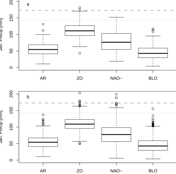
BLO), we determined the conditional probability distribution of January precipitation in Southern UK when a weather regime frequency exceeds 75% of the month. Figure 4 shows that only ZO and NAO− weather regimes reach the record values observed in January 2014. A dominant zonal weather regime obviously increases the risk of high precipitation in the winter, al-though extreme precipitations can also be reached with the NAO− pattern. The horizontal dashed lines (observed precipitation vs. 99th quantile of W1) suggest that the Weather@Home simulations might underestimate monthly precipitation rates.
10
This shows that the North Atlantic circulation patterns are discriminating for heavy precipitation in Southern UK. Hence we focus on the zonal and NAO− atmospheric patterns to compute the probability changes.
3.2 Reanalyses and observations
The world W1is made of the NCEP reanalysis data for the winters (December to February) between 1951 and 2016 (Kalnay et al., 1996). It is the “new” world. The world W0is made of the 20CR reanalysis data for the winters between 1900 and 1950
15
(Compo et al., 2011). It is the “old" world.
Those two reanalyses use different models, assimilation schemes and assimilated data. Schaller et al. (2016, Suppl. infor-mation) showed that the weather regime classification in the overlapping period of the two reanalyses are very similar. We also verify that the analogues of January 2014 are qualitatively similar in the two reanalyses over the 1950–2011 period. For each day of January 2014, the 20 best analogues have between 12 and 18 days in common in the two reanalyses. The distances and
20
spatial correlation yield probability distributions that cannot be distinguished by a Kolmogorov-Smirnov test (von Storch and Zwiers, 2001).
The circulation C is taken from the SLP of both reanalyses. The precipitation R is taken from daily precipitation observations from the UK Met Office (Matthews et al., 2014) between 1900 and 2014. The dataset consists of observations from 14 stations in the southern UK. The variable R is a monthly average of daily values of those stations. We verify that a record of precipitation
25
was reached in January 2014 (Fig. 5).
The weather regimes were computed on a reference period (1970 – 2000) in the NCEP reanalysis, with a k-means algorithm (Yiou et al., 2008) (Fig. 1). We checked for consistency that the weather regimes of the 20CR reanalysis are the same as for NCEP, as well as the regime frequencies ((Schaller et al., 2016, Suppl. Information)). After a removal of the mean, the SLP of Weather@Home simulations is projected onto those reference centroids to compute the weather regime frequencies. This is
30
done to ensure the consistency of the interpretation of the regime frequencies.
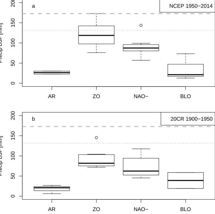
Since high values of precipitation R can be obtained with more than one weather regime (namely, the zonal and NAO− regimes) (Figs. 4 and 6), the decomposition of Eq. (2) is repeated for those two weather regimes.
Again, the North Atlantic circulation patterns are discriminating for heavy precipitation in Southern UK. Hence we focus on the zonal and NAO− atmospheric patterns to compute the probability changes.
● ● ● ● ● ● ● ●
AR
ZO
NAO−
BLO
0
50
100
150
200
J
an. Precip [mm]
a
● ● ● ● ● ● ● ● ● ● ● ● ● ● ● ● ● ● ● ● ● ● ● ● ● ● ● ● ● ● ● ● ● ● ● ● ● ● ● ● ● ● ● ● ●AR
ZO
NAO−
BLO
0
50
100
150
200
J
an. Precip [mm]
b
Figure 4. January precipitation probability distribution (boxplots) conditional to winter weather regimes exceeding 75% in Weather@Home
simulations (panel a: W1factual world; panel b: W0counterfactual world). The thin dashed horizontal line is the 99% quantile of the W1
1900
1920
1940
1960
1980
2000
1
2
3
4
5
Year
SUK Precip [mm/da
y]
●
Figure 5. Time series of January mean daily observed precipitation in Southern UK between 1900 and 2014 (in mm/day). The red dot indicates the value of R for January 2014.
●
AR
ZO
NAO−
BLO
0
50
100
150
200
Precip DJF [mm]
NCEP 1950−2014
a
●AR
ZO
NAO−
BLO
0
50
100
150
200
Precip DJF [mm]
b
20CR 1900−1950
Figure 6. Cumulated Southern UK January precipitation (in mm) probability distribution conditional to winter weather regimes exceeding
75% in reanalyses (panel a: NCEP; panel b: 20CR). The thin dashed horizontal line is the 99% quantile of W1(NCEP). The thick dashed
4 Results
4.1 Weather @ Home
The ρ ratios were computed from the (≈17000) factual and (≈117000) counterfactual Weather@Home simulations. Since p1 is fixed to be 0.01 (for a return period of one century), the spread of ρ stems from the uncertainty on p0that is computed
5
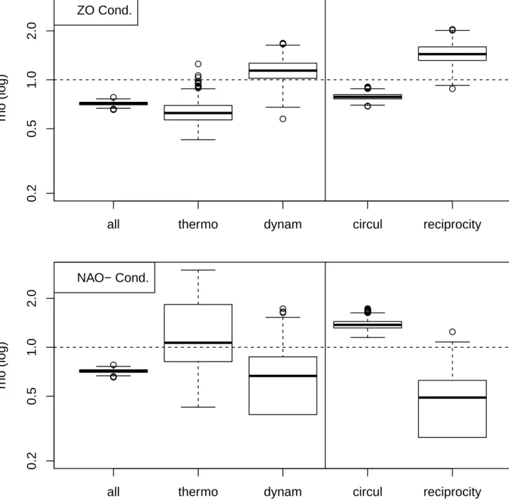
over the pooled counterfactual simulations. The distribution of ρ is significantly different from 1, with a mean value ¯ρ = 0.71. This indicates an increase of the risk of heavy precipitation in W1 with respect to W0, with a fraction of attributable risk (FAR = 1 − p0/p1) of 0.29. The estimates of ρthe, ρcirc, ρrecfor the zonal and NAO− are shown in Figure 7. By construction, the products of the mean values recover the mean value of ρ.
The three mean ratios ( ¯ρthe, ¯ρcirc, ¯ρrec) are significantly different from 1 for the zonal regime ( ¯ρthe≈ 0.63, ¯ρcirc≈ 0.78 and
10
¯
ρrec≈ 1.45). The thermodynamical contribution with the zonal contribution (1 − ¯ρthe) is about ≈ 1.7 times ((1; 2.5) with a 80% confidence interval) the dynamical contribution (1 − ¯ρcirc), which is coherent with the estimate of Schaller et al. (2016), who find a thermodynamic contribution twice as large as the dynamic contribution, with a different approach. The ρthe< 1 is interpreted by an increase of precipitation from W0to W1given the same weather regime flow. ρcirc< 1 reflects an increase of the frequency of zonal patterns in W1with respect to W0. ρrec> 1 reflects that large precipitation amounts occur more often
15
during episodes of zonal circulation.
The NAO− yields a quite different picture. The ρtheratio is not distinguishable from 1 and has a large variability. Therefore it cannot be concluded that this weather regime has a significant thermodynamic contribution to changes of heavy precipitation rates. ¯ρcirc> 1 means that the mean January precipitation rate decreases for NAO− from W0to W1. The reciprocity ratio ¯ρrec is lower than 1, meaning that NAO− is less likely during episodes of high precipitation. This means that the NAO− regime
20
becomes less frequent and less rainy, in contradistinction to the zonal regime.
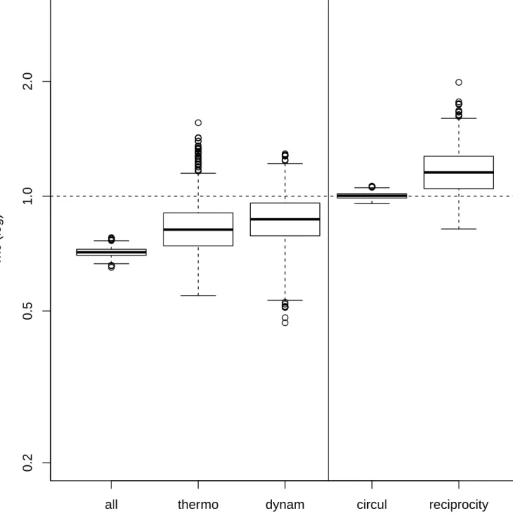
An analogue-like approach was used to estimate the ρ decomposition from the Weather@Home data. The distance between the January 2014 SLP in NCEP and each Weather@Home simulation was computed, as the average of daily SLP distances. Then the neighborhood of Cref= CJan.2014 is defined when this average distance is lower than a threshold estimated from analogues of NCEP data. The value of the threshold is 1.5 times the average (over January 2014) of the median of the distances
25
of the 20 best daily analogues. This leads to a threshold value of 12 hPa and defines the “circulation tube” of Section 2.3.2. In this way, the conditional probabilities (and their probability density functions (pdf)) can be estimated by bootstrapping. The pdf of each probability ratio are shown in Figure 8.
We see that the thermodynamical contribution is very similar to the one of the zonal circulation pattern in Figure 7, but the dynamical contribution has an opposite sign. The circulation contribution is ≈ 1, indicating that the probability of having a
30
circulation like the one of January 2014 does not change significantly, while the reciprocity term is lowered. Therefore, the frequency of a persisting zonal weather regime increases between the counterfactual and factual worlds, while probability of having a circulation history that is similar to 2014 remains stable. This apparent contradiction is explained by the fact that the circulation of January 2014, although zonal, was rather dissimilar to the usual zonal weather regime. Hence, by tightening the
● ● ● ● ● ● ● ● ● ● ● ● ● ● ● ● ● ● ● ● ● ● ● ● ● ● ● ● ● ● ● ● ● ● ● ● ● ● ●
all
thermo
dynam
circul
reciprocity
0.2
0.5
1.0
2.0
rho (log)
ZO Cond.
● ● ● ● ● ● ● ● ●●●●●●●●●●●●●●●●●●●●●● ●all
thermo
dynam
circul
reciprocity
0.2
0.5
1.0
2.0
rho (log)
NAO− Cond.
Figure 7. Changes in probability ratios from weather regimes in Weather@Home simulations. The probability ratios (vertical axes) are shown on a logarithmic scale. The horizonal dashed lines show the reference ρ = 1 line. The dynamical contribution is the product of the circulation and reciprocity contributions. The upper panel is the conditional probability ratios for the Zonal regime. The lower panel is for the NAO− regime.
● ● ● ● ● ● ● ● ● ● ● ● ● ● ● ● ● ● ● ● ● ● ● ● ● ● ● ● ● ● ● ● ● ● ● ● ● ● ● ● ● ● ● ● ● ● ● ● ● ● ● ● ● ● ● ● ● ● ● ● ● ● ● ● ● ● ● ● ● ● ● ● ● ● ● ● ● ● ●
all
thermo
dynam
circul
reciprocity
0.2
0.5
1.0
2.0
rho (log)
Figure 8. Changes in probability ratios from the analogue approach in Weather@Home simulations. The probability ratios (vertical axes) are shown on a logarithmic scale. The horizonal dashed lines show the reference ρ = 1 line. The dynamical contribution is the product of the circulation and reciprocity contributions.
class of event from “high precipitation sum due to zonal weather regime” to “high precipitation sum due to a specific persisting circulation”, we change the quantification of a dynamical contribution.
This emphasizes the need of a precise definition of the neighborhood of a circulation trajectory for the conditional attribution exercise. On the one hand, one looks at a persisting zonal circulation in a rather broad sense. On the other hand, one looks at a
5
circulation trajectory that looks like the observation of January 2014, which yielded an atypical zonal pattern (van Oldenborgh et al., 2015).
4.2 Reanalyses
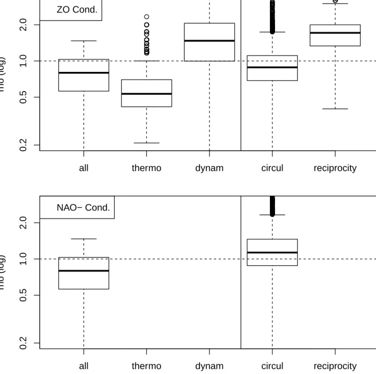
Similar estimates of ρ, ρthe, ρcirc and ρrec were computed from the NCEP (W1 from 1951 to 2015) and 20CR (W0 from 1900 to 1950) reanalyses (Figure 9). The mean ratio ¯ρ is ≈ 0.82 ((0.51; 1.12) with a 80% confidence interval), indicating a
10
FAR value of ≈ 0.18. The distribution of ρ is marginally significantly different from 1, but its range is compatible with the Weather@Home estimate.
The three ratio distributions (ρthe, ρcirc, ρrec) were computed for the zonal and NAO− weather regimes (Figure 9).
The mean values are marginally different from 1 for the zonal regime ( ¯ρthe≈ 0.61, ¯ρcirc≈ 0.93 and ¯ρrec≈ 1.76). This description is qualitatively similar to what was obtained with the Weather@Home analysis, although the magnitudes differ, due
15
to the differences between the two universes (factual vs. counterfactual, and new vs. old). The uncertainty increase is partly due to the limited lengths of the reanalysis datasets. The thermodynamical contribution with the zonal contribution (1 − ¯ρthe) is about ≈ 6.4 times the dynamical contribution (1 − ¯ρdyn). If a confidence interval of the ratio (1 − ¯ρthe)/(1 − ¯ρdyn) is built upon the bootstrap samples for which ρtheand ρcircare lower than 1, then we obtain an 80% interval of (0.70; 7.98). Such a procedure is necessary because ρcircexceeds 1 with a probability larger than 0.3. The mean reciprocity ratio ¯ρrec is rather
20
close to what was found in the Weather@Home analysis. It indicates an increase of zonal circulation when heavy precipitation occurs between the beginning of the 20th century and the present-day period.
The ρ ratio distributions for the NAO− regime are not very informative. The thermodynamic and reciprocity contributions cannot be estimated because the threshold of precipitation is never reached during a winter dominated by NAO− in the NCEP reanalysis, between 1951 and 2016, implying zero denominators in Eq. (3, 5). A first interpretation is that the NAO− regime
25
is so different in both worlds that the conditional precipitation change cannot be estimated (because Pr(R(1)> Rref|C(1)∈ V(Cref)) = 0 and Pr(C(1)∈ V(Cref)|R(1)> Rref) = 0). This might be due to the low number of winters in the W0world (i.e. 50 years).
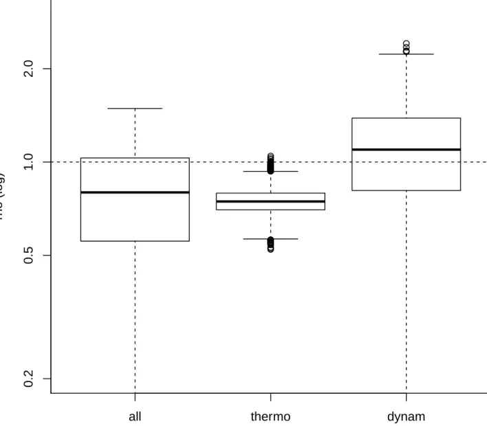
The ratio distributions with the analysis of SLP analogues is shown in Figure 10. The distribution of ρtheis sharper than with the weather regime description due to the tighter constraint on the shape of the atmospheric trajectory. The dynamical
30
term ρdynis barely above 1 (contrary to the ZO weather regime in the same worlds), although not significantly.
This apparent contradiction is explained by the fact that the ZO weather regime becomes slightly more probable in W1than in W0(circulation term in Figure 9), but the average distance of SLP analogues of January 2014 slightly increases between W0and W1(Figure 11). This reflects the fact that the January 2014 pattern is not a typical zonal pattern (as seen in Figure 2) and that the thermodynamical term outbalances the dynamical term in the interpretation of ρ < 1.
● ● ● ● ● ● ● ● ● ● ● ● ● ● ● ● ● ● ● ● ● ● ● ● ● ● ● ● ● ● ● ● ● ● ● ● ● ● ● ● ● ● ● ● ● ● ● ● ● ● ● ● ● ● ● ● ● ● ● ● ● ● ● ● ● ● ● ● ● ● ● ● ● ● ● ● ● ● ● ● ● ● ● ● ● ● ● ● ● ● ● ● ● ● ● ● ● ● ● ● ● ● ● ● ● ● ● ● ● ● ● ● ● ● ● ● ● ● ● ● ● ● ● ● ● ● ● ● ● ● ● ● ● ● ● ● ● ● ● ● ● ● ● ● ● ● ● ● ● ● ● ● ● ● ● ● ● ● ● ● ● ● ● ● ● ● ● ● ● ● ● ● ● ● ● ● ● ● ● ● ● ● ● ● ● ● ● ● ● ● ● ● ● ● ● ● ● ● ● ● ● ● ● ● ● ● ● ● ● ● ● ● ● ● ● ● ● ● ● ● ● ● ● ● ● ● ● ● ● ● ● ● ● ● ● ● ● ● ● ● ● ● ● ● ● ● ● ● ● ● ● ● ● ● ● ● ● ● ● ● ● ● ● ● ● ● ● ● ● ● ● ● ● ● ● ● ● ● ● ● ● ● ● ● ● ● ● ● ● ● ● ● ● ● ● ● ● ● ● ● ● ● ● ● ● ● ● ● ● ● ● ● ● ● ● ● ● ● ● ● ● ● ● ● ● ● ● ● ● ● ● ● ● ● ● ● ● ● ● ● ● ● ● ● ● ● ● ● ● ● ● ● ● ● ● ● ● ● ● ● ● ● ● ● ● ● ● ● ● ● ● ● ● ● ● ● ● ● ● ● ● ● ● ● ● ● ● ● ● ● ● ● ● ● ● ● ● ● ● ● ● ● ● ● ● ● ● ● ● ● ● ● ● ● ● ● ● ● ● ● ● ● ● ● ● ● ● ● ● ● ● ● ● ● ● ● ● ● ● ● ● ● ● ● ● ● ● ● ● ● ● ● ● ● ● ● ● ● ● ● ● ● ● ● ● ● ● ● ● ● ● ● ● ● ● ● ● ● ● ● ● ● ● ● ● ● ● ● ● ● ● ● ● ● ● ● ● ● ● ● ● ● ● ● ● ● ● ● ● ● ● ● ● ● ● ● ● ● ● ● ● ● ● ● ● ● ● ● ● ● ● ● ● ●
all
thermo
dynam
circul
reciprocity
0.2
0.5
1.0
2.0
rho (log)
ZO Cond.
● ● ● ● ● ● ● ● ● ● ● ● ● ● ● ● ● ● ● ● ● ● ● ● ● ● ● ● ● ● ● ● ● ● ● ● ● ● ● ● ● ● ● ● ● ● ● ● ● ● ● ● ● ● ● ● ● ● ● ● ● ● ● ● ● ● ● ● ● ● ● ● ● ● ● ● ● ● ● ● ● ● ● ● ● ● ● ● ● ● ● ● ● ● ● ● ● ● ● ● ● ● ● ● ● ● ● ● ● ● ● ● ● ● ● ● ● ● ● ● ● ● ● ● ● ● ● ● ● ● ● ● ● ● ● ● ● ● ● ● ● ● ● ● ● ● ● ● ● ● ● ● ● ● ● ● ● ● ● ● ● ● ● ● ● ● ● ● ● ● ● ● ● ● ● ● ● ● ● ● ● ● ● ● ● ● ● ●all
thermo
dynam
circul
reciprocity
0.2
0.5
1.0
2.0
rho (log)
NAO− Cond.
Figure 9. Changes in probability ratios in 20CR/NCEP reanalyses for the zonal and NAO− weather regimes. The probability ratios (vertical axes) are shown on a logarithmic scale. The horizonal dashed lines show the reference ρ = 1 line. The dynamical contribution is the product of the circulation and reciprocity contributions. The upper panel is the conditional probability ratios for the Zonal regime. The lower panel is for the NAO− regime. There are no thermodynamical or reciprocity terms in the decomposition because high precipitation sums do not occur during persisting NAO− episodes in 1900–1950.
● ● ● ● ● ● ● ● ● ● ● ● ● ● ● ● ● ● ● ● ● ● ● ● ● ● ● ● ● ● ● ● ● ● ● ● ● ● ● ● ● ● ● ● ● ● ● ● ● ● ● ● ● ● ● ● ● ● ● ● ● ● ● ● ● ● ● ● ● ● ● ● ● ● ● ● ● ● ● ● ● ● ● ● ● ● ● ● ● ● ● ● ● ● ● ● ● ● ● ● ● ●
all
thermo
dynam
0.2
0.5
1.0
2.0
rho (log)
● ● ● ● ● ● ● ● ● ● ● ● ● ● ● ● ● ● ● ● ● ● ● ● ● ● ● ● ● ● ● ● ● ● ● ● ● ● ● ● ● ● ● ● ● ● ● ● ● ● ● ● ● ● ● ● ● ● ● ● ● ● ● ● ● ● ● ● ● ● ● ● ● ● ● ● ● ● ● ●
DJF dist(j,2013/2014) [hP
a]
● ● ● ● ● ● ● ● ● ● ● ● ● ● ● ●5
6
7
8
9
10
11
20CR
NCEP
Figure 11. Distribution of mean distances (in hPa) between Winter 2013/2014 and the 20 best analogues in NCEP and 20CR. The black boxplot are for the whole winter (DJF) and the red boxplot are for January 2014 only.
The analogue method does not allow for an estimate of the circulation and reciprocity terms because we are only able to sample trajectories around January 2014, not all trajectories like in the Weather@Home experiments.
5 Discussion
We have performed analyses on two different world definitions (“factual” vs. “counterfactual” and “new” vs. “old”). There is
5
no quantitative way of claiming that factual equals new and counterfactual equals old. It is only possible to argue qualitatively that the anthropogenic forcings were weaker in the “old” world than in the “new” world.
One of the caveats of attribution studies (including this one) is the uncertainty in the W0 world, which affects estimates of p0. This problem exists in the “counterfactual” simulations of Weather@Home, which required the subtraction of an SST signal from 11 available CMIP5 simulations. Each of the invidual counterfactual simulations show different behavior, although
10
the ensemble yields a significant, albeit small, change with respect to W1, as shown by Schaller et al. (2016). The quality and quantity of the data that was used in the reanalysis experiments varies with time. This implies that the “old” world is more uncertain that the “new” world. The distributions of distances between analogues in Figure 11 do not show large systematic biases in 20CR (1900–1950) with respect to NCEP (1950–2016). Using the whole ensemble of 20CR could allow for better estimates of weather regime frequency distributions in the W0 world, but the only precipitation data we used come from
15
observations, which means that uncertainties in the ρ ratio are always large. Another possibility is to consider subperiods of 1900–1950, but the confidence for individual subperiods is bound to be very poor.
The analysis does not consider internal temporal variability in each world. The Weather@Home simulations do not have decadal variability, but reanalyses do. This was not taken into account here, but could be included by further dividing the two worlds (“old” versus “new”) into subperiods (e.g. “high SST” versus “low SST”) in order to evaluate the feedback of natural
20
SST variability on atmospheric circulation. This poses the problem of the length of available data onto which the statistics are built. This difficulty could be overcome by investigating ensembles of available simulations such as CMIP5 (Taylor et al., 2012) or CORDEX (Jacob et al., 2013).
The main assumption made in the Bayesian decomposition is that the climate variable R is related to the atmospheric circulation field C, and that a storyline of C can explain an observed extreme of R. This ensures that the two conditional
25
probabilities in Eq. (2) are non zero so that the ratios are well defined.
In order to provide consistent results, it is necessary to have a correct representation of the atmospheric variability. This assumption is not trivial and required many verifications on the Hadley Center atmospheric model (Schaller et al., 2016). The circulation patterns that were simulated were validated over the North Atlantic region and Europe for the W1factual world. The main difficulty is that there is no way to assess the validity of C in the W0counterfactual world. This is where the assumption
30
that W1and W0are close to each other is heuristically used in the estimate of the probability changes. Of course, this is not a strict proof of validation of the atmospheric circulation in W0.
When reanalysis data are used, the question of the atmospheric circulation validity and the R–C relation is tied to the quality of the data that are used in the assimilation scheme, for both worlds W0and W1. The main caveat is that the early period
of reanalyses are constrained by only a few observations (Compo et al., 2011). This means that the circulation reconstruction could yield wrong patterns (even for the members of the ensemble), with no possible validation test. The second caveat in this case is the length of datasets on which the probabilities are computed. Moreover, the observed climate (or its reanalysis) is one occurrence of many possible realizations that could have happened for a given climatic state. Therefore this analysis should
5
also be understood as being conditional to a dataset (either Weather@Home or the earlier part of the 20CR reanalysis), which is an uncertain representation of the world.
Our paper outlined an apparent discrepancy between weather regime and analogues of circulation to describe thermodynam-ical changes (and dynamthermodynam-ical ones). Weather regimes offer a rather rough description of the atmospheric flow and the range of possible flows within a weather regime classification can be fairly large. The recent winter of 2015/2016 pleads for a finer
de-10
scription of the atmospheric circulation. Indeed, December 2015 had a mostly zonal weather regime (like January 2014), with very mild temperatures in Europe, but southern UK and northwestern France were very dry (like the rest of continental Europe), while northern UK experienced record precipitation and floods. The jet stream was slightly shifted (a few hundred kilometers) to the north, but the weather regime was still zonal, while having no resemblance to January 2014 (in terms of analogues). This questions the focus of extreme event attribution on regional climate precipitation alone, as already discussed by Trenberth et al.
15
(2015), since the large-scale atmospheric circulation that drives the moisture transport can have shifts within the same weather regime and hit a region rather than its neighbors just by chance. This suggests an EEA analysis of the predictands of R (like C), rather than R alone, with a focus on the dynamical terms.
Vautard et al. (2016) proposed an alternative method based on analogues to determine dynamical and thermodynamical components from the Weather@Home simulation data. It is interesting to notice that there is a consensus on the estimate of
20
a thermodynamical term (i.e. with equal atmospheric circulation). Our finding emphasizes that a definition of a dynamical contribution is potentially still ambiguous. We also emphasize that the approach of analogues can also be applied to daily Weather@Home data (Figure 8). Vautard et al. (2016) investigated all possible patterns of atmospheric circulation on a monthly time scale, while this study focuses on January 2014, with a daily time scale.
The persistence of events and hence the time scale to be considered are major components to be considered. For instance,
25
the probabilities of having a persistent zonal weather regime during a month and having a circulation that is similar to January 2014 have different distributions, and such distributions change in different ways between the two reanalysis datasets. Such a consideration is crucial for regional climate studies: as mentioned above, the example we chose in this paper is about precip-itation in southern UK (and arguably northwestern France which also had records of precipprecip-itation in January 2014). But case studies like northern UK (in December 2015) or Wales in 2000 (Pall et al., 2011) would require separate analyses because the
30
difference in atmospheric flows is different in a subtle but crucial way.
It is desirable to be systematic in the attribution of extreme events in continuous time, by examining all events. This pleads for analyses that can be performed quickly in order to diagnostics in a relatively short time. This can help guide the choice of heavier experiments such as Weather@Home in order to refine estimates.
6 Conclusions
We have argued that the use of relatively short datasets (reanalyses) provide qualitatively similar information in terms of prob-ability decomposition of the occurrence of a winter flood event. Such an analysis cannot replace Weather@Home simulations in order to quantify precisely the contribution of all factors. Therefore the second exercise (with reanalyses) is a detection
5
rather than a thorough attribution, as defined by Bindoff et al. (2013). The attribution comes if the forcing changes are clearly identified in both periods, which is not done in this paper.
The names of terms (thermodynamical and dynamical) of the decomposition can be debated. It is important to note that changes in the properties of the atmospheric circulation C and the coupling between the local climate variable R and C play an important role in the definition of the extreme event.
10
The conditional part of the analysis is the most important point as it helps to explore the tail of the distribution of R. We emphasize that we analyze a high precipitation rate (R > Rref) conditional to a given circulation pattern Cref. We had to make the analysis of the two types of weather regimes leading to high precipitation rates. The thermodynamical and dynamical contributions differed from one weather regime to the other.
We also emphasize that the paradigm of attribution of extreme events that we have explored can also be applied to other
15
contexts, in particular extreme events of the last millennium as a response to solar and volcanic forcings (Schmidt et al., 2011, 2014; Bothe et al., 2015). This can be done by exploring analogues of circulation of a given extreme event in remote periods (in model simulations) where natural forcings are well documented.
Author contributions. TEXT
Acknowledgements. It is a pleasure to thank Ted Shepherd (U Reading) for useful discussions. PY is supported by the ERC grant No.
20
References
Allen, M.: Liability for climate change, Nature, 421, 891–892, 2003.
Bindoff, N., Stott, P., AchutaRao, K., Allen, M., Gillett, N., Gutzler, D., Hansingo, K., Hegerl, G., Hu, Y., Jain, S., Mokhov, I., Overland, J., Perlwitz, J., Sebbari, R., and Zhang, X.: Detection and Attribution of Climate Change: from Global to Regional, pp. 867–952, Cambridge
5
University Press, Cambridge, United Kingdom and New York, NY, USA, 2013.
Bothe, O., Evans, M., Donado, L., Bustamante, E., Gergis, J., Gonzalez-Rouco, J., Goosse, H., Hegerl, G., Hind, A., Jungclaus, J., Kaufman, D., Lehner, F., McKay, N., Moberg, A., Raible, C., Schurer, A., Shi, F., Smerdon, J., Von Gunten, L., Wagner, S., Warren, E., Wid-mann, M., Yiou, P., and Zorita, E.: Continental-scale temperature variability in PMIP3 simulations and PAGES 2k regional temperature reconstructions over the past millennium, Clim. Past, 11, 1673–1699, doi:10.5194/cp-11-1673-2015, 2015.
10
Cattiaux, J., Vautard, R., Cassou, C., Yiou, P., Masson-Delmotte, V., and Codron, F.: Winter 2010 in Europe: A cold extreme in a warming climate, Geophys. Res. Lett., 37, doi:10.1029/2010gl044 613, 2010.
Christidis, N. and Stott, P.: Extreme rainfall in the United Kingdom during winter 2013/14: The role of atmospheric circulation and climate change, Bull. Amer. Met. Soc., 96, S46–S50, doi:10.1175/BAMS-D-15-00094.1, 2015.
Compo, G., Whitaker, J., Sardeshmukh, P., Matsui, N., Allan, R., Yin, X., Gleason, B., Vose, R., Rutledge, G., Bessemoulin, P., Brönnimann,
15
S., Brunet, M., Crouthamel, R., Grant, A., Groisman, P., Jones, P., Kruk, M., Kruger, A., Marshall, G., Maugeri, M., Mok, H., Nordli, O., Ross, T., Trigo, R., Wang, X., Woodruff, S., and Worley, S.: The Twentieth Century Reanalysis Project, Quarterly J. Roy. Meteorol. Soc., 137, 1–28, doi:10.1002/qj.776., 2011.
Hannart, A., Pearl, J., Otto, F., Naveau, P., and Ghil, M.: Causal counterfactual theory for the attribution of weather and climate-related events, Bull. Amer. Meteorol. Soc., 97, 99–110, 2016.
20
Huntingford, C., Marsh, T., Scaife, A. A., Kendon, E. J., Hannaford, J., Kay, A. L., Lockwood, M., Prudhomme, C., Reynard, N. S., Parry, S., Lowe, J. A., Screen, J. A., Ward, H. C., Roberts, M., Stott, P. A., Bell, V. A., Bailey, M., Jenkins, A., Legg, T., Otto, F. E. L., Massey, N., Schaller, N., Slingo, J., and Allen, M. R.: Potential influences on the United Kingdom’s floods of winter 2013/14, Nature Clim. Change, 4, 769–777, 2014.
Jacob, D., Petersen, J., Eggert, B., Alias, A., Christensen, O. B., Bouwer, L. M., Braun, A., Colette, A., Déqué, M., Georgievski, G.,
Geor-25
gopoulou, E., Gobiet, A., Menut, L., Nikulin, G., Haensler, A., Hempelmann, N., Jones, C., Keuler, K., Kovats, S., Kroner, N., Kotlarski, S., Kriegsmann, A., Martin, E., Meijgaard, E., Moseley, C., Pfeifer, S., Preuschmann, S., Radermacher, C., Radtke, K., Rechid, D., Roun-sevell, M., Samuelsson, P., Somot, S., Soussana, J.-F., Teichmann, C., Valentini, R., Vautard, R., Weber, B., and Yiou, P.: EURO-CORDEX: new high-resolution climate change projections for European impact research, Region. Env. Change, pp. 1–16, doi:10.1007/s10113-013-0499-2, 2013.
30
Kalnay, E., Kanamitsu, M., Kistler, R., Collins, W., Deaven, D., Gandin, L., Iredell, M., Saha, S., White, G., Woollen, J., Zhu, Y., Chelliah, M., Ebisuzaki, W., Higgins, W., Janowiak, J., Mo, K., Ropelewski, C., Wang, J., Leetmaa, A., Reynolds, R., Jenne, R., and Joseph, D.: The NCEP/NCAR 40-year reanalysis project, Bull. Amer. Met. Soc., 77, 437–471, 1996.
Kimoto, M. and Ghil, M.: Multiple flow regimes in the Northern-hemisphere winter. 1. Methodology and hemispheric regimes, J. Atmos. Sci., 50, 2625–2643, 1993.
35
Massey, N., Jones, R., Otto, F. E. L., Aina, T., Wilson, S., Murphy, J. M., Hassell, D., Yamazaki, Y. H., and Allen, M. R.: weather@home—development and validation of a very large ensemble modelling system for probabilistic event attribution, Quat. J. Roy. Met. Soc., 141, 1528–1545, doi:10.1002/qj.2455, 2015.
Matthews, T., Murphy, C., Wilby, R. L., and Harrigan, S.: Stormiest winter on record for Ireland and UK, Nature Clim. Change, 4, 738–740, 2014.
Michelangeli, P., Vautard, R., and Legras, B.: Weather regimes: Recurrence and quasi-stationarity, J. Atmos. Sci., 52, 1237–1256, 1995. National Academies of Sciences Engineering and Medicine, ed.: Attribution of Extreme Weather Events in the Context of Climate Change,
5
The National Academies Press, Washington, DC, doi:10.17226/21852, 2016.
Pall, P., Aina, T., Stone, D. A., Stott, P. A., Nozawa, T., Hilberts, A. G. J., Lohmann, D., and Allen, M. R.: Anthropogenic greenhouse gas contribution to flood risk in England and Wales in autumn 2000, Nature, 470, 382–385, doi:10.1038/Nature09762, 2011.
Peixoto, J. P. and Oort, A. H.: Physics of climate, American Institute of Physics, New York, 1992.
Schaller, N., Kay, A. L., Lamb, R., Massey, N. R., van Oldenborgh, G. J., Otto, F. E. L., Sparrow, S. N., Vautard, R., Yiou, P., Ashpole,
10
I., Bowery, A., Crooks, S. M., Haustein, K., Huntingford, C., Ingram, W. J., Jones, R. G., Legg, T., Miller, J., Skeggs, J., Wallom, D., Weisheimer, A., Wilson, S., Stott, P. A., and Allen, M. R.: Human influence on climate in the 2014 southern England winter floods and their impacts, Nature Clim. Change, 6, 627–634, 2016.
Schmidt, G., Annan, J., Bartlein, P., Cook, B., Guilyardi, E., Hargreaves, J., Harrison, S., Kageyama, M., Legrande, A., Konecky, B., Love-joy, S., Mann, M., Masson-Delmotte, V., Risi, C., Thompson, D., Timmermann, A., and Yiou, P.: Using palaeo-climate comparisons to
15
constrain future projections in CMIP5, Clim. Past, 10, 221–250, doi:10.5194/cp-10-221-2014, 2014.
Schmidt, G. A., Jungclaus, J. H., Ammann, C. M., Bard, E., Braconnot, P., Crowley, T. J., Delaygue, G., Joos, F., Krivova, N. A., Muscheler, R., Otto-Bliesner, B. L., Pongratz, J., Shindell, D. T., Solanki, S. K., Steinhilber, F., and Vieira, L. E. A.: Climate forcing reconstructions for use in PMIP simulations of the last millennium (v1.0), Geoscientific Model Development, 4, 33–45, 2011.
Shepherd, T. G.: A Common Framework for Approaches to Extreme Event Attribution, Current Climate Change Reports, 2, 28–38,
20
doi:10.1007/s40641-016-0033-y, 2016.
Stott, P. A., Stone, D. A., and Allen, M. R.: Human contribution to the European heatwave of 2003, Nature, 432, 610–614, doi:10.1038/Nature03089, 2004.
Stott, P. A., Christidis, N., Otto, F. E. L., Sun, Y., Vanderlinden, J.-P., van Oldenborgh, G. J., Vautard, R., von Storch, H., Walton, P., Yiou, P., and Zwiers, F. W.: Attribution of extreme weather and climate-related events, Wiley Interdisciplinary Reviews: Climate Change, 7, 23–41,
25
doi:10.1002/wcc.380, 2016.
Taylor, K. E., Stouffer, R. J., and Meehl, G. A.: An Overview of CMIP5 and the Experiment Design, Bull. Amer. Met. Soc., 93, 485–498, 2012.
Trenberth, K. E., Fasullo, J. T., and Shepherd, T. G.: Attribution of climate extreme events, Nature Clim. Change, 5, 725–730, 2015. van Haren, R., van Oldenborgh, G. J., Lenderink, G., and Hazeleger, W.: Evaluation of modeled changes in extreme precipitation in Europe
30
and the Rhine basin, Envir. Res. Lett., 8, 014 053, 2013.
van Oldenborgh, G. J., Stephenson, D. B., Sterl, A., Vautard, R., Yiou, P., Drijfhout, S. S., von Storch, H., and van den Dool, H.: Drivers of the 2013/14 winter floods in the UK, Nature Clim. Change, 5, 490–491, 2015.
Vautard, R., Legras, B., and Déqué, M.: On the source of midlatitude low-frequency variability. 1. A Statistical approach to persistence, J. Atmos. Sci., 45, 2811–2843, 1988.
35
Vautard, R., Yiou, P., Otto, F., Stott, P., Christidis, N., van Oldenborgh, G. J., and Schaller, N.: Attribution of human-induced dynamical and thermodynamical contributions in extreme weather events, Envir. Res. Lett., accepted, 2016.
Yiou, P.: AnaWEGE: a weather generator based on analogues of atmospheric circulation, Geoscientific Model Development, 7, 531–543, doi:10.5194/gmd-7-531-2014, 2014.
Yiou, P. and Nogaj, M.: Extreme climatic events and weather regimes over the North Atlantic: When and where?, Geophys. Res. Lett., 31, doi:10.1029/2003GL019119, 2004.
Yiou, P., Goubanova, K., Li, Z., and Nogaj, M.: Weather regime dependence of extreme value statistics for summer temperature and
precipi-5
tation, Nonlin. Proc. Geophys., 15, 365–378, 2008.
Yiou, P., Salameh, T., Drobinski, P., Menut, L., Vautard, R., and Vrac, M.: Ensemble reconstruction of the atmospheric column from surface pressure using analogues, Clim. Dyn., 41, 1333–1344, doi:10.1007/s00382-012-1626-3, 2013.