The relevance of the cross-wavelet transform in the analysis of human interaction -a tutorial

HAL Id: hal-02432769

https://hal.umontpellier.fr/hal-02432769

Submitted on 8 Jan 2020

HAL is a multi-disciplinary open access

archive for the deposit and dissemination of

sci-entific research documents, whether they are

pub-lished or not. The documents may come from

teaching and research institutions in France or

abroad, or from public or private research centers.

L’archive ouverte pluridisciplinaire HAL, est

destinée au dépôt et à la diffusion de documents

scientifiques de niveau recherche, publiés ou non,

émanant des établissements d’enseignement et de

recherche français ou étrangers, des laboratoires

publics ou privés.

analysis of human interaction -a tutorial

Johann Issartel, Thomas Bardainne, Philippe Gaillot, Ludovic Marin

To cite this version:

Johann Issartel, Thomas Bardainne, Philippe Gaillot, Ludovic Marin. The relevance of the

cross-wavelet transform in the analysis of human interaction -a tutorial. Frontiers in Psychology, Frontiers,

2015, 5, pp.1566. �10.3389/fpsyg.2014.01566�. �hal-02432769�

The relevance of the cross-wavelet transform in the

analysis of human interaction – a tutorial

Johann Issartel1_{*, Thomas Bardainne}2_{, Philippe Gaillot}3 _{and Ludovic Marin}4

1_{Multisensory Motor Learning Laboratory, School of Health and Human Performance, Dublin City University, Dublin, Ireland} 2_{Geophysics Imagery Laboratory, Université de Pau et des Pays de l’Adour, Pau, France}

3

ExxonMobil Upstream Research Company, Hydrocarbon Systems Division, Structure, Petrophysics & Geomechanics, Houston, TX, USA 4

Movement to Health Laboratory, Sciences et Techniques des Activités Physiques et Sportives, EuroMov, University Montpellier 1, Montpellier, France

Edited by:

Holmes Finch, Ball State University, USA

Reviewed by:

Pietro Cipresso, IRCCS Istituto Auxologico Italiano, Italy

Holmes Finch, Ball State University, USA

*Correspondence:

Johann Issartel, Multisensory Motor Learning Laboratory, School of Health and Human Performance, Dublin City University, Collins Avenue, Glasnevin, Dublin 9, Ireland

e-mail: johann.issartel@dcu.ie

This article sheds light on a quantitative method allowing psychologists and behavioral scientists to take into account the specific characteristics emerging from the interaction between two sets of data in general and two individuals in particular. The current article outlines the practical elements of the cross-wavelet transform (CWT) method, highlight-ing WHY such a method is important in the analysis of time-series in psychology. The idea is (1) to bridge the gap between physical measurements classically used in physiology – neuroscience and psychology; (2) and demonstrates how the CWT method can be applied in psychology. One of the aims is to answer three important questions WHO could use this method in psychology, WHEN it is appropriate to use it (suitable type of time-series) and HOW to use it. Throughout these explanations, an example with simulated data is used. Finally, data from real life application are analyzed. This data corresponds to a rating task where the participants had to rate in real time the emotional expression of a person. The objectives of this practical example are (i) to point out how to manipulate the properties of the CWT method on real data, (ii) to show how to extract meaningful information from the results, and (iii) to provide a new way to analyze psychological attributes.

Keywords: cross-wavelet transform, relative phase, human interaction, plurifrequential time-series, joint action

INTRODUCTION

In psychology, numerous studies investigate the interactions between different components of a living system or between dif-ferent living systems. The idea of interaction is meant here as the expression of action that occurs as two or more ‘objects’ have an effect upon one another (Sebanz and Knoblich, 2009). Numerous studies in psychology also investigate the progression in time of these interactions (Boyd et al., 2011). The data set obtained when analyzing human interaction, and even more when analyzing the temporal evolution of human interaction, contains a lot of pow-erful information, which is sometimes difficult to quantify and interpret. The cross-wavelet1transform (CWT) method offers a way to overcome such difficulties. The ‘cross’ WT method is a technique that characterizes the interaction between the wavelet transform (WT) of two individual time-series. Even if the pur-pose of this tutorial is essentially based on a description of the interaction between time-series (i.e., the CWT method), some explanations will refer to the WT method when the method-ological explanations are not focused on the interaction between time-series.

The core of this tutorial will be mainly based on practical expla-nations rather than reviewing, once more, all mathematics behind those techniques. Readers interested by mathematical details can refer to “A practical guide on time-frequency analysis to study human motor behavior: the contribution of WT” byIssartel et al. (2006)or they can refer to a tutorial in neuroscience fromSamar 1_{The term wavelet means a small wave.}

et al. (1999), or in psychology fromIhlen and Vereijken (2010). Various application of the WT can be found in psychophysiology (Frantzidis et al., 2014), in the analysis of event-related potentials for Schizophrenic patients (Roth et al., 2007) and behavioral neu-roscience (Inoue and Sakaguchi, 2014;Schmidt et al., 2014). The illustrations will be based on both synthetic and real data sets. Step by step, we aim to demonstrate the advantages of the CWT in psychology for non-experts in signal processing research. Our purpose is to describe and illustrate the relevance of the CWT method (and the associated tools) to study the interaction phe-nomenon between different components of a living system or between different living systems. By the end the article the reader should have an understanding of the strength and advantage of the CWT method and be able to evaluate the benefits of this method on his/her experimental signals. The mathematical aspects will not be detailed in this tutorial. Such a description would be the topic of another article. We deliberately kept our focus on how to understand the potential use of the CWT method and on how to extract the useful information when analyzing time-series in psychology.

These interaction phenomena are permanently present in our everyday life. Such ubiquity implies that all psychological fields are involved in the study of interaction phenomena and most of them tend to use time-series analyses. For instance, in social psychology Gernigon et al. (2004) demonstrate that in sport, states of involvement toward mastery, performance-approach, and performance-avoidance goals flow, are temporally interrelated. Clinical studies also examine the interaction phenomenon. For

instance,Slewa-Younan et al. (2004)illustrated the difference in brain functional connectivity between males and females with schizophrenia. In the wide field of behavioral studies, one can find numerous cases of research on interaction phenomena using time-series analyses. For example, in human communication lis-teners mirror the movements of a storyteller (Bavelas et al., 1988;

Voutilainen et al., 2014), in music, body movement (e.g., foot tapping) is coordinated with the melody (Jones, 1993), and also in human conversational interaction (Boker and Rotondo, 2002;

Guastello et al., 2005;Pincus and Guastello, 2005;Kupetz, 2014), in the development of infant joint attention and social cognition (Mundy and Jarrold, 2010), in collective behavior organization like rapturous applause (Neda et al., 2000), or even in handwriting when a synchronization phenomenon appears between the rhyth-mic movement of the fingers and the wrist (Sallagoïty et al., 2004). The above list of studies, focusing on the interaction phenomena, is obviously not exhaustive. Other examples will be presented, in this article, while introducing the core components of the CWT method.

The concept of interaction refers to a synchronization phe-nomenon (Kelso, 1995, for a review) between the elements that compose a system or between different systems (Moraru et al., 2005).Moraru et al. (2005)defined the general synchronization phenomenon as the characterization and quantification of inter-dependencies between different system components. The term synchronization is a construct used in numerous fields to denote the temporal relationship between events. This relationship occurs in a variety of contexts, for example, when sport fans start a wave across a stadium, when two people emotionally “click” with one another (e.g., parent–infant synchrony –Granic and Lamey, 2002), or the sleep–wake rhythm with the light–dark cycle. There is not only synchronization when two components are perfectly coordinated (such as two soldiers in lockstep – i.e., in phase with each other), but as long as any kind of interac-tion exists between two (or more) components. In such a context, although it seems paradoxical, two ex-partners opposed while divorcing, synchronize their actions. When partner 1 makes a deci-sion, partner 2 frequently contradicts partner 1. In this example, they both “move” in the same time but in the opposite direc-tion (anti-phase). This synchronizadirec-tion phenomenon can also be observed, on a daily basis, when friends mimic each other posture and even speech patterns while sipping coffee. In this context, synchronization occurs with certain latency that is also a common characteristic when systems are interacting with each other.

The CWT method allows us (i) to measure the degree of synchronization phenomenon between different components and conjointly (ii) the evolution over time of the studied phenomenon (i.e., times-series data set). For example, it allows the extraction of information about how a behavioral state changes, how long it takes to progress from one state to another and how many states occur in a given time period. In addition, similarity/differences between two time-series (e.g., the similarity between two peo-ple’s behavioral states) can be identified. If these behavioral states do not have a similar dynamic (i.e., different temporal evolu-tion), the CWT method helps quantifying how different they are, and what is the time lag between the two different behavioral

states? In short, this method is able to yield information on the spatio-temporal organization between two time-series, or in other words how two time-series evolve one against the other. We will address different examples based either on synthetic or real data sets to demonstrate how this method can be helpful to interpret time-series.

This tutorial is organized in an accessible way for readers with different backgrounds. First of all, we demonstrate WHAT the WT is and how it is related to the notions of synchronization and relative phase (RP). Secondly, we explain WHY the analyses performed with this method could offer a beneficial way to inter-pret time-series data obtained from psychological experiments. In the third section, we subsequently illustrate WHO could use this method. In other words, which areas in psychology could potentially benefit from using this method. The fourth section is dedicated to an explanation of the time-series specificities required to use this method (called the “WHEN” section). We explore the types of time-series that could be used and those that seem to present some limitations. Then, we detail the WT method using a synthetic example to illustrate HOW this method can be applied on time-series data set and HOW to extract useful information. Throughout this section, we associate a synthetic example with a psychologically concrete related example to contextualize this method for the reader. Finally, a real set of data is analyzed. The data has been taken from an experiment assessing the dynamics of emotional state. The idea is to analyze this real time-series from the extraction of the variables up to the interpretation phase of the results.

WHAT IS THE CROSS-WAVELET TRANSFORM METHOD? As stated in introduction, the notion of synchronization plays a key role in the understanding of the CWT method. First of all, we will define the concept of synchronization. We will demonstrate how the synchronization is related to two other elements, namely the RP and the frequency. These explanations will constitute the fundamental knowledge needed to understand the CWT method.

SYNCHRONIZATION

As described earlier on, the synchronization phenomenon can be considered as an ongoing relationship between different structures or systems. The systematic study of this experimental as well as the-oretical phenomenon has been widely investigated in physics since

Appleton (1922)andvan der Pol(1927; for a review, Pikovsky et al., 2003), but was only introduced in experimental psychology byKelso (1981)in the theoretical framework of coupled dynamical systems. This dynamical system can be applied to understand-ing appraisal or emotion for example. Nowadays many scientists will consider emotion as non-linear, dynamic, distributed where self-organized patterns emerge from the interaction between the components of a system. This spontaneous emergence of order, coherence and synchronization have been examined and ana-lyzed with different methods (e.g., the windowed cross-correlation function, Boker et al., 2002). Although, there are multiple ways to observe the correlation or the coherency between two com-ponents, only one variable can describe and precisely measure the phase synchrony between different components. The phase synchrony, also called the RP, is a variable commonly applied to

psychology because it conveys the essential aspects of a behavior by summarizing the relations between the components of a sys-tem. It examines the relationships between spatial and temporal information.

RELATIVE PHASE

Traditionally, measures of RP have been used to quantify the coor-dination between two or more components during an activity (seeKelso, 1995, for a review) as well as to determine the tran-sition from one behavior to another either intentionally (Scholz and Kelso, 1990) or unintentionally (Kelso, 1981) such as two gaits unintentionally synchronized when two partners are walk-ing in the street side by side. The RP can be understood as a relational variable that measured the ordering of the interaction among components. The self-organized interaction between com-ponents leads to the emergence of a behavioral dynamics. In other words, the RP capture the coordination between the components. A coordination where the components are moving in the same direction, at the same time, have a RP of 0◦ (also called in-phase) while a coordination with a phase shift of 180◦ is called anti-phase.

For instance,Kelso (1981)analyzed the coordination/coupling between two fingers and quantified phase relationships as the dif-ference between successive flexions or extensions in the oscillations of the fingers. This approach is called the point estimate of the RP (seeVon Holst, 1973) and corresponds to a discrete relative phase (DRP). The DRP computes the RP between two time-series as the temporal difference between two inflection points in the time-series. For example, in a dynamic measurement of psycho-logical states, like states of goal involvement toward mastery and performance-avoidance goals flow (Gernigon et al., 2004), it is pos-sible to measure a reference point each time the states are changing direction (i.e., the inflection point between the end of the increas-ing state of involvement toward mastery and the beginnincreas-ing of the decreasing of this state). Psychological momentum is considered as a dynamical phenomenon defined as “a positive or negative dynamics of cognitive, affective, motivational, physiological, and behavioral responses (and their couplings) to the perception of movement toward or away from either an appetitive or aver-sive outcome” (Gernigon et al., 2010, p. 397). In this citation, the key words – positive/negative or appetitive/aversive – high-light to the notion of continuous dynamical changes occurring in the coupling between components. The interactions between cognitive vs. physiological or affective vs. motivational compo-nents, in a given situation, are on constant evolution (up and down, slow or fast, etc. . .). In the study byGernigon et al. (2010), they manipulated the scenarios of performance in a table ten-nis match by increasing or decreasing the scores gaps between players. They assessed the anxiety or self-confidence levels of a participant observing the video of a match. They were interested in understanding how the perception of moving toward or away from the desired outcome (winning) affect the above mentioned psychological determinants. They measured these determinants after each point during the match. This discrete measurement provides a snapshot of these determinants in a sequential basis (point-to-point) but does not take into account how determi-nants such as expectations of success, anxiety, perceived situational

threat evolve from moment-to-moment2_{. The RP between two of} these psychological determinants would capture the behavioral dynamics between these components. In such a case, the RP could provide, for example, an expression of the spatio-temporal orga-nization between two goal involvement states. This DRP method can be applied to a time-series with changes in frequency (e.g., slow increases vs. fast decreases of self-confidence) and amplitude (minor vs. major changes) and allows us to describe the evolution of the RP as a function of time. However, the DRP only computes one or two measures of RP per cycle (i.e., time between two inflec-tion points). Therefore, the DRP does not provide a continuous estimation of the variability of the RP, or an accurate estimation of the time of occurrence of a transition (i.e., when the behavior switches from one state to another). This is crucial information while studying participants’ behavioral modifications. To remedy these limitations, another method of computing the continuous relative phase (CRP) between two time-series has been developed (Kelso, 1995).

While the DRP gives one or two values of RP per cycle, the CRP provides the RP for every point of the time-series. This higher resolution gives a more accurate picture of phase transi-tion, for example, the moment of transition from one behavioral state to another can be quantified (seeKelso et al., 1987). One of the most famous methods used to analyze the continuous RP is called the Hilbert transform, which provides higher resolution results than the DRP methods (Fuchs et al., 1996;Rosenblum et al., 1996,2001). This method gives both the instantaneous phase and amplitude of the time-series, which is an advantage because with one method, it is possible to measure both the amplitude and the RP of time-series. Mathematically speaking, this method can be used for non-harmonic and non-stationary time-series. For these reasons, this methodology has been successfully applied in behav-ioral psychology in order to detect phase synchronization between two non-stationary time-series corresponding, for instance, to the displacement of two tennis players (Palut and Zanone, 2004) or to get an accurate measure of the time of intentional switches from one graphic pattern to another in a handwriting task (Sallagoïty et al., 2004).

So far, the Hilbert transform seems to be a relevant method to detect the phase synchronization between two time-series pro-viding that the components of the time-series possess the same frequencies (e.g., similar time of variation between the two state involvement goals). However, this method cannot be directly applied to the analysis of the phase synchronization between two plurifrequential components of a time-series. A plurifre-quential time-series is composed of a time-series with multiple frequencies occurring in the same time as it is commonly the case in living systems. For instance while a pigeon is walking, if we observe the movements of the head, we would notice two frequencies: one frequency triggered by the pigeon’s gait and a second one caused by the rhythmical forward and backward movements of the head, commonly called head-bobbing (Frost, 1978; Green et al., 1994; Troje and Frost, 2000). Let’s consider

2_{Using a ‘mouse-paradigm’ which consisted in moving a computer mouse to}

track participants moment-to-moment self-evaluation based on their own recorded narrative.

another example based on the dynamics of self-esteem (Ninot et al., 2005) to illustrate the idea of plurifrequential time-series. These authors studied the dynamics of self-esteem over a 6-months period. The results revealed a short history dynamic adjustment of self-esteem, which corresponds to frequency mod-ulations of time-series in a short period of time (such as per day). They also discussed the possibility of another dynamic of self-esteem over a longer period of time. This hypothesis suggests the common presence of short-term and long-term dependencies of self-esteem. In other words, participants have demonstrated short-term adjustments of their self-esteem (time-scale= day) imbricated within long-term adjustments (time-scale= month-year). This indicates plurifrequential components in the self-esteem time-series. The CWT method would be able to deal with such plurifrequential time-series and is conjointly able to detect the phase synchronization of such time-series. The next section will be dedicated to an explanation of the interrelation between the notion of frequency and the notion of RP in time-series, which will facilitate an understanding of how the CWT method works.

THE RELATIVE PHASE AND FREQUENCY RELATIONSHIP

A simple way to illustrate the interdependence between the notion of frequency and RP is to use a practical example – an enacted series of knock-knock jokes. In this dual situation, most of the sentences are controlled and set. For example, the joke always starts with the teller saying: ‘knock-knock’ (first utterance) and the responder answering ‘who’s there?’ (second utterance). The main objective forSchmidt et al. (2012)was to understand better the behavioral synchronization occurring in social interaction dur-ing structured conversation. Their finddur-ings revealed the presence of two “behavioral waves” (i.e., two frequencies) when analyzing a series of 10 consecutive jokes: one of these frequencies corre-sponding to the time-scale of the utterances and the other one corresponding to the time-scale of the joke. A synchronous syn-ergy (i.e., RP) was observed between the two participants when looking at the utterances time-scale (in-phase). When looking at the joke time-scale, a lag was observed between the teller and the responder with the teller leading the behavioral interaction (RP≈40◦). This experimentation illustrates that, in the context of social interaction, the behavior can be nested in several tem-poral scales (plurifrequential time-series). Each of these scales contributes to the emergence of human communication inter-action. In this example, the interaction required 0◦of phase on one frequency and 40◦of phase on the other frequency. The joint analysis of both time (frequency) and space (RP) provides the foundation to better understanding the structure of coordinated actions.

As illustrated in the above example, the notions of RP is intrin-sically related to the notion of frequency. Understanding the time-series characteristics is essential in the identification of the frequency (or the period) components and consequently crucial when it comes to analyzing the RP (Fuchs et al., 1996; Sternad et al., 1999a,b;Rosenblum et al., 2001;Peters et al., 2003;Pikovsky et al., 2003; Kano and Kinoshita, 2010). In that sense, the CWT method takes into account both frequency and RP components of the analyzed time-series.

WHY DOES IT SEEM IMPORTANT TO USE THE CROSS-WAVELET TRANSFORM METHOD?

As discussed above, classical methods (DRP and Hilbert trans-form) break down when the time-series are composed of two or more main frequency components [plurifrequential time-series – see examples on (i) short-term and long-term adjustment of the self-esteem or (ii) the knock-knock jokes]. Such situations are well suited to the CWT method because it does not require any hypothesis about the nature of the series. Complex time-series having frequency, amplitude, and/or phase modulations do not prevent the use of the WT method. The analyzable time-series could evolve in a random way without any consequences on the results. It would typically be the case if we had to analyze the dynamic of self-esteem. The short-term dynamic adjustment can appear and disappear over time without influencing the analysis of the long-term dynamic adjustment (Ninot et al., 2005). The two levels of analysis can be performed independently. Therefore, the frequency, amplitude or RP modulations at one level do not affect the results of the other levels of analysis. Moreover, having the possibility to get the RP for each of the frequencies provides complementary information. The RP results for the knock-knock experiment at the joke time-scale offers a better understanding of the leader-follower relationship with a specific quantification of the time-lag between the joke teller and the responder. Each of the frequency and RP characteristics specific to the CWT method will be discussed in the section “HOW.” The objective of the following section is to highlight WHO is currently using the CWT method and to whom it could be extended to in several psychological domains.

WHO IS USING THE RELATIVE PHASE AND THE CROSS-WAVELET TRANSFORM METHOD?

The CWT method has been applied in diverse scientific domains as mathematics, engineering science and more recently in physiol-ogy (Sakowitz et al., 2001;De Carli et al., 2004;Rezaei et al., 2008) and neuroscience (Herreras et al., 1994; Rodriguez et al., 1999;

Armand and Minor, 2001;Cao et al., 2010; Westin et al., 2010). In psychology some studies used the WT method to examine ver-bal or non-verver-bal sounds (Rendalla et al., 2007;Uclés et al., 2009), recognition of emotional facial expression (Knyazev et al., 2008) or interpersonal motor coordination (Issartel et al., 2007; Ashen-felter et al., 2009;Schmidt et al., 2014). The interested readers will find resources introducing the CWT method in methodological articles or books (Chui, 1992a,b;Daubechies, 1992;Burrus et al., 1998; Torrence and Compo, 1998; Mallat, 1999; Walker, 1999;

Percival and Walden, 2000; Le Van Quyen et al., 2001; Addison, 2002;Fugal, 2009).

WHO COULD USE THE RELATIVE PHASE AND THE CROSS-WAVELET TRANSFORM METHOD?

The RP offers several opportunities to investigate time-series in psychology. For this a reason, RP could now be used in many psychological fields to characterize human behavior. It could be applied to different kinds of human phenomena from synchronization between systems within a single human (e.g., locomotor respiratory coupling,Villard et al., 2005), to inter-limb co-ordination (e.g., the index finger of the two hands,Haken et al.,

1985), or interaction between personality characteristics such as self-confidence, performance goal flow (Gernigon et al., 2002– see detailed explanation in Section “Relative Phase”). The lat-ter research group have analyzed the dynamics of psychological momentum from an actor or an observer perspectives in order to deeply investigate the moment-to-moment variations of a given variable (Briki et al., 2013,2014). Using the CWT method, this research group could have reached similar goals while also being able to perform a complementary series of experimentation. The positive and negative psychological momentums could be manip-ulated and consequently compared to the dynamics of affective or motivational components. Along the same line, the study by

Avugos et al. (2013)investigating the role of self-efficacy on ath-letic performance could benefit from the current method as they could analyze the interaction between performance outcomes and self-efficacy beliefs over time. Other application domains could also be found in sport or in daily situations at work between a line manager and employees for example. It seems also important to consider the dynamics of learning as a potential application area for the CWT method. For example, the relationship between developmental dynamics of mathematical performance (Aunola et al., 2004) and cognitive, motivational, or achievement-related task-avoidant behavior (Hirvonen et al., 2012) variables. In the context of social psychology, the relationship between a buyer and a supplier for example can be considered from the cyclical attraction process angle (Ellegaard, 2012). Industrial marketing research is interested in uncovering the features and process of attraction to understand better the close ties between customers and suppliers. In this context, the CWT method could contribute in quantifying specifically this interpersonal relationship in analyz-ing people behaviors or communication strategies over time and observed whether there were several levels (that we call frequen-cies here) that triggered different behaviors. Social psychologists have also investigated dyadic situation in the development of anti-social behavior (Granic and Lamey, 2002;Granic and Patterson, 2006). Using the space space grid (SSG), they were able to quan-tify, in real time, observational data of two participants (Lewis et al., 1999). This methodology allowed them to identify specific conditions drawing the dyadic behavior toward hostile or cooper-ative behavior. An analysis of these oscillatory behaviors over time with the CWT method would be complementary to this analysis (e.g., hostile≈180◦and cooperative≈0◦of RP) with a quantifi-cation of the time lag (or latency) between the two participants behavioral response as well as an estimation of the speed of the response.

More widely, the CWT could also be applied in psychiatry to observe mental disorders as altered neuronal organizations in the brain (Peled, 2005), or to give insight into chronic schizophrenia (Slewa-Younan et al., 2004) or even in interpersonal motor coor-dination to understand how two people synchronize with each other (Schmidt et al., 1998; Richardson et al., 2005). In light of the above, other fields in psychology not currently using the RP and/or the CWT method may see the purpose of doing so in the future (Riley and Holden, 2012). The next section will be dedicated to the question of “WHEN” in order to exemplify the kind of data that should be considered as suitable for the CWT method.

WHEN CAN WE USE THIS METHOD?

CATEGORICAL vs. CONTINUOUS SCALES

Categorical data can be sorted according to a discrete category. The first type of categorical data is nominal data. Nominal data is named or labeled without any regard to the value of the obser-vation. In a nominal set of data the values associated with the observation are not measured. For this reason, nominal data cannot be used with the CWT method. The second type of categorical data is ordinal data. An ordinal set of data has a nat-ural order, therefore the values can be ranked but the difference between neighboring points on the scale may differ. The CWT method can only be applied on a set of data having constant differences/intervals between two adjacent observations.

Continuous data scales refer to scales where the interval between observations (sampling rate) is constant. All kinds of continuous data can be analyzed with the CWT method.

WHAT HAPPENS IF DATA ARE MISSING?

The WT and the CWT cannot be applied in the case of missing data in a time-series. Either data have to be re-collected or imputation methods can be used to fill in the missing data. At this stage, one need to identify what are the best imputation methods to use. With regard to this, an extensive literature is available (for a review see

Little and Rubin, 2002). The authors strongly recommend extreme caution in the use of any kind of imputation strategy keeping in mind the possibility of potentially biased interpretations.

ARE THERE DURATION BOUNDARIES FOR THE ANALYSES?

The minimum duration of the time-series depends on the lowest frequency (longest period) of the time-series (i.e., the slowest set of data to be analyzed). Based on this knowledge, the minimum dura-tion of the time-series analyzed is twice the duradura-tion of the lowest frequency. Let’s take the example of a study on the dynamic of self-esteem with the assumption that the long-term modulations correspond to a period of 2 months. Therefore, one should mea-sure the dynamic of the self-esteem once a month during 4 months (see Minimum Sampling Rate). In terms of the maximum dura-tion of the time-series to analyze, there is mathematically no boundary.

MINIMUM SAMPLING RATE

The minimum sampling rate (or sampling frequency) recom-mendation is based on the Nyquist–Shannon sampling theorem. The lowest bound for the sampling rate has to be two times the highest frequency of the time-series. For example, if the fastest behavior observed occurs every 2 s then the highest frequency is 0.5 Hz (Frequency= 1/Period). Therefore, two times the min-imum sampling rate of 0.5 Hz is 1 Hz. To illustrate this point, we could take the example of the enacted knock-knock exper-imentation from Schmidt et al. (2014). The highest observed frequency for this experiment was based on the utterance time-scale (i.e., 1.33 Hz). Based on the Nyquist–Shannon sampling theorem, the minimum sampling rate should be 2.66 Hz. The actual sampling rate they used was almost six times faster (i.e., 15 Hz). In this situation, this sampling rate guarantees a fine temporal accuracy for the RP analyses. Overall, the sampling rate should be maintained throughout the duration of any given

experiment. If it is not the case, interpolation methods should be used.

DOES THE SAME SET OF CRITERIA APPLY FOR CWT AND WT METHOD? For both the WT and CWT methods, the same criteria apply. For a valid comparison between two time-series, the CWT analysis requires the same duration for the two time-series and a similar sampling rate. Downsampling methods may be useful if one of the two time-series has a higher sampling rate than the other.

The next section will be dedicated to a step-by-step description of HOW it is possible to use the CWT method.

HOW TO USE THE WAVELET TRANSFORM METHOD

This step-by-step presentation of the WT will explain the key ele-ments of the WT method in a comprehensive treatment. The mathematical aspect of the method is not in the scope of this tutorial. The description will allow the reader to understand the elements in order to apply the method him/herself. When the reader has an understanding of the following keys elements, he/she will be ready to apply this method on their own signals using the wavelet toolbox of the Matlab software (MathWorks Inc., Nat-ick, MA, USA). Readers can also use the code currently utilized for the analyses in this article as well as a “Cook-book” on how to use and understand the code. The code can be downloaded at the fol-lowing address: ‘http://webpages.dcu.ie/ issartej/WavePackage.zip’ INTRODUCTION TO SPECTRAL METHODS

The Fourier transform (FT) is a method transforming a time-series from the time domain to the frequency domain. This spectral analysis provides a global description of the frequency content of a given time-series (for more details on the application of the FT method in psychology seeVallacher and Nowak, 1994). When we want to understand when (temporal dimension) an event occurs in a time-series, the analysis in the frequency domain independently of the temporal domain cannot provide a satisfactory answer (Flandrin, 1988). Consequently, methods have been developed to take into account both time and frequency content of a time-series. The most logical and well-known method is the Windowed FT (WFT) based on the FT method itself. But instead of analyz-ing the full time-series, the FT is performed on short consecutive (overlapping or not) segments. The moving/translating windows allow for the detection of sudden changes in the frequency content of the time-series. The main limitation of this method is the lack of precision to either the time or the frequency domain. The size of the segment will determine either a high level of precision in the time domain or in the frequency domain. For example, a small window would not allow for the detection of any event larger than the window while maintaining a good localization in time. On the other end, a large window will take into account the long-term event (frequency domain) but with a high level of imprecision in the temporal domain.

A further methodological development of the WFT led a way to compare two time-series together. The cross-WFT (CWFT) can evaluate the interactions between 2 time-series providing infor-mation about the common frequency content between them as well as the difference in phase at a given frequency. It is important to note that the limitation presented above for the FT method also

apply to the CFT method. Overall, highlighting these two methods is central to this article, as they constitute the foundation stones of the further development of WT and the CWT3.

ORIGINS OF THE WAVELET TRANSFORM METHOD

Historically, the WT method was introduced in seismic research byMorlet (1983). Since then, wavelets are commonly used in geo-sciences (seeKumar and Foufoula-Georgiou, 1997for a review) as they are particularly well-suited in characterizing the “local” properties of time-series. The meaning of “local” has to be understood as the opposite of “global.” As mentioned in the previous section, the “global” properties of a time-series refer to an average/summary of the time-series properties not tak-ing into account the evolution of these properties over-time. The WT method will characterize the “local” properties of the time-series. Each occurrence of the time-series will be taken into account in the analysis. Due to these properties, the WT has been the object of various methodological developments and numerous applications in scientific domains as detailed in the section WHO.

FUNDAMENTAL KEY STEPS OF THE WAVELET TRANSFORM METHOD

The WT method is based on a FT analysis. As discussed in Section “Introduction to Spectral Methods,” the FT is not able to detect temporal discontinuities or yield information on the temporal persistence of periodicities. The conjoint characterization and quantification of each frequency component in time must be taken into consideration as does the characterization and the quan-tification of the associated RP. This joint characterization of the frequency content of the time-series in time while keeping a high level of precision in both time and frequency domains consti-tutes one of the WT advantages. The exploration of the frequency range of interest as a function of time results in a “time-scale” or time-frequency representation (2D map) of the time-series. This time-frequency representation could be compared to a piece of music (that represents the time-series) written as a musical score. Each musical note could be represented by a frequency parame-ter (y-axis) and by the time of occurrence (x-axis). Before, we go into a deeper explanation of the method, we will explain what a time-frequency representation (or time-frequency plane) is.

TIME-FREQUENCY PLANE

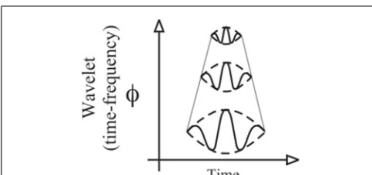
The time-frequency plane is the graphical representation used to illustrate the results obtained with the WT and the CWT method. This time-frequency plane contains the same information as the original time-series but expressed in another way: in frequency as a function of time. The time-frequency plane is defined by (i) the frequency that ranges from zero to the Nyquist frequency (i.e., 1/2δ(t), where δ(t) is the sampling interval – see section WHEN) and (ii) the time spans of time-series. As illustrated inFigure 1, the time-frequency-plane is tiled with rectangular tiles, usually called Heisenberg cells. The area of each cell is dictated by the uncertainty principle. This principle illustrates the necessary trade-off, in the calculations, between the accuracy in time and in frequency that influence consequently the accuracy of the phase calculation. A

3_{For more detailed explanations about the cross-spectral methods please refers to}

FIGURE 1 | Tiling of the time-frequency plane for the wavelet transform (WT) method. Narrow rectangles are used for the high frequencies that give a precise localization in time. Large rectangles are used for the low frequencies that give a precise localization in frequency. This illustrates the trade-off between the accuracy in time and the accuracy in frequency.

better resolution in the time domain triggers a diminution in the frequency resolution and vice-versa.

For the study of the WT, Flandrin (1988) called the time-frequency plane a scalogram. In a scalogram, the time-scale of the rectangle is flexible (c.f. Figure 1). Narrow rectangles are used for the high frequencies that give a precise localization in time. Large rectangles are used for the low frequencies that give a precise localization in frequency. Thus, the scalogram possesses multi-scale structures that allow us to precisely define the temporal and the frequency locations and to perform a multi-scale analysis (Torrence and Compo, 1998). Each of these structures contains an analyzing function (details about this function will be provided below) used during the computation to analyze the properties of the time-series. The modification of the size (dilation/contraction) of this analyzing function over time (translation) provides the key in quantifying the frequency and the RP location of the time-series (Figure 2).

DILATATION/CONTRACTION/TRANSLATION OF THE ANALYZING FUNCTION

The WT is calculated by convolving the time-series s(t) with an analyzing wavelet functionψ(a, b) (derived from a mother func-tionψ) by dilatation of a and translation of b. The variable a

FIGURE 2 | Representation of the contraction/dilatation of the analyzing function in the time-frequency plane.

is the scale factor that determines the characteristic frequency so that varying a gives rise to a spectrum; b is the translation in time so that variable b represents the “sliding window” of the wavelet over s(t) – see Flowchart (step 2). Concerning the scale factor a, the analyzing wavelet function is swept over the whole time-series for the frequency ranges as a function of time. Because the WT method is naturally bound and invariant by translation, it is par-ticularly suited for a local analysis. According to the frequencies analyzed, the analyzing function is either dilated or contracted. Thus, the tiling of the time-frequency plane depends on the con-traction/dilatation of the analyzing function (Figure 2). Hence, the WT method is also invariant by contraction/dilatation, allow-ing multi-scale analysis (Figure 2). These properties offer a good trade-off in both time and frequency domains (Torrence and Compo, 1998;Percival and Walden, 2000).

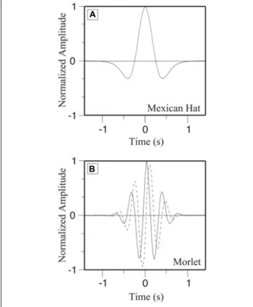
Mathematically a great number of analyzing functions (see examples Figure 3) could be created (Torrence and Compo, 1998). The choice of the analyzing function is neither unique nor arbitrary and mostly dependent on the likeness between the time-series and the analyzing function. Specific descriptions and recommendations of the properties of the analyzing function can be found in the literature (e.g.,Torrence and Compo, 1998;

Mallat, 1999;Fugal, 2009). We recommend to the interested read-ers to refer to this literature before starting the analysis of their time-series.

The best way to understand these principles is by examining an example based on easily understandable time-series. To do so, two synthetic time-series were created. The two time-series, s1

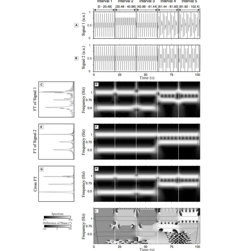
(Figure 4A) and s2(Figure 4B) have a duration of 102.4 s (with a sampling rate of 50 Hz). The amplitude of s1and s2is 1 arbitrary unit (a.u.). Both time-series have been divided into five intervals. For the first three intervals [0–61.44], the time-series are com-posed of a high frequency component at 1 Hz and a low frequency component at 0.5 Hz. For the last two intervals [61.44–102.4], the time-series are composed of a high frequency component (1 Hz) and an intermediate frequency component (0.75 Hz). The first interval is characterized by a zero degree RP between s1 and s2 (the two time-series are identical in this interval). In interval 2, the time-series s1is characterized by a 90◦ phase lag in the high frequency component (1 Hz) whereas a 90◦phase lag is applied on s1in the low frequency component (0.5 Hz) of the third interval. In the fourth interval, a phase lag of 90◦ on the high frequency component and a phase lag of 180◦on the intermediate frequency component are applied to s1. In the fifth interval, a phase lag of 180◦on the high frequency component and of 90◦on the inter-mediate frequency component are applied to s1(see Table 1 for a summary of the changes made to s1). Note that no phase lag exists in s2.

The above description of the synthetic time-series could be potential hard to relate to a“real”example. To facilitate the reading, we propose to describe this time-series as if it was a moment-to-moment and/or a day-to-day dyad interaction between a parent and a child. This dynamical interaction constantly evolves with several time-scales: from short-term interactions (e.g., dual tasks) to long-term interactions (i.e., week-to-week, year-to-year). On this basis, interval 1 would represent a high synergy (0◦ RP) between the parent (s1) and the child (s2). The shift to a 90◦degree

FIGURE 3 | Temporal representation of (A) the Gaussian (Mexican Hat) and (B) the Morlet analyzing functions.

RP in interval 2 would be associated with some sort of latency from one of the participants in reaction to the other participant’s behav-ior. In an ongoing situation, when an unpredicted event occurs, it induces a dysregulation of the interaction. This could trigger anger or sadness to a child. In this context, the latency (90◦RP) could be explained, for example, by a delayed response/reaction of the parent to the child’s anger. After a given time (interval 3), the short-term interaction between the parent and the child goes back to a high level of synchrony (0◦of RP) with a knock-on effect on the long-term interaction (90◦RP for the low frequency). Intervals 4 and 5 at the short-term interaction level indicates a deteriora-tion of the reladeteriora-tionship up to a point (180◦ of RP) where the parent and the child behaviors are going in the opposite direction. This behavioral shift could also be observed on the longer-time scale (Intervals 4 and 5). This seems to indicate the bidirectional nature of the interaction across the different time-scales. If we were to interpret these results, one will suggest that the short-term and long-short-term interactions are influencing each other with potential consequences for (i) the person itself (e.g., developmen-tal outcome) and his/her environment (e.g., friends and family). In the following section, we will regularly refer to this example to illustrate the key aspects of the CWT method.

Figures 4A,B represent the amplitude of time-series 1 (s1) and time-series 2 (s2) respectively on the Y-axis as a function of time. Figures 4C,E,G represent the FT spectra of s1and s2respectively as well as the cross-FT. From these two types of representation (time vs. frequency), it is very difficult to quantify differences,

similarities or interactions between these two time-series. By visu-ally inspecting the time-representation of s1and s2(Figures 4A,B) it is clear that something happened at the beginning of intervals 2 and 4 (e.g., sudden modification of the nature of the interaction between the parent and the child), but it is impossible to relate these changes to modifications in the frequency dynamics. On the other hand, a comparison of the Fourier spectra (Figures 4C,E,G) informs us that s1and s2 contain three main frequency compo-nents. But these spectra do not provide any information about how these frequency components evolve with time (i.e., when this sudden interaction changes occur). The WT time-frequency rep-resentation of the two time-series (Figures 4D,F) provides both the temporal and frequency information. We can see such a rep-resentation in Figures 4D,F that represent the WT spectrum of s1 and s2respectively.

The previous explanations constitute a necessary first step in the understanding of (i) the WT method and more specifically (ii) the time-frequency representation. The information contained in the time-frequency representation has to be quantified in order to perform statistical analysis.

STATISTICAL TEST TO DISCRIMINATE THE PROPERTIES OF TIME-SERIES (SEE FLOWCHART STEP 4)

Hence, from the CWT method, we obtain an expression of the whole range of frequency as a function of time. In order to quantify and use the results of the WT, statistical analysis can be applied. The first objective is to determine the frequencies statistically present in the WT spectrum (also called a scalogram). The statistical test used in this article is based on the test used byTorrence and Compo (1998). These authors have demonstrated that, each point of the WT spectrum is statistically distributed as a chi-square with two degrees of freedom. The confidence level is computed as the prod-uct of the background spectrum (the power at each scale) by the desired significance level from the chi-square (χ2_{) distribution.}

When the WT spectrum is higher than the associated confidence level it is said to be “statistically significant.” If the background spectrum is not known, one should use, as recommended by the latter authors, the global wavelet spectrum (time-average of the wavelet spectrum) as background. By extension, Torrence and Compo (1998)established the confidence levels of a cross-wavelet spectrum (see next section) from the square root of the product of two chi-square distributions. The confidence level is determined classically at the desired level (in this article we used 95% confi-dence). The set of statistically significant coefficients is a matrix of numbers that it is possible to extract for further quantitative analysis.

In Figures 4D,F,H,I the thin black lines outline statistically significant zones defined from the statistical test proposed by Tor-rence and Compo (1998). As we previously explained, the WT permits us to detect the time where the frequency modification appears. From the top to the bottom ofFigure 4D, it is clear that in the three first intervals [0–61.44] we can see, firstly a white band that represents the high frequency component at 1 Hz (short-term adjustments) and secondly the white band that represents the low frequency component at 0.5 Hz (long-term adjustments). For the first three intervals, Figures 4D,F are exactly the same except at the beginning of each interval for Figure 4D due to influences

FIGURE 4 | Wavelet transform analysis and cross-wavelet transform (CWT) analysis of time-series (s1and s2). (A,B) are the representations

of s1and s2, respectively; (C,E) show the normalized Fourier spectrum of

(A,B), respectively. In both cases, we can observe one main peak at 1 Hz and two other peaks at 0.75 Hz and 0.5 Hz. (D,F) are WT spectra (scalograms) of (A,B) respectively. These figures help to localize and quantify in terms of time of localization (time) and amplitude the frequency components previously identified in the Fourier spectra. In (D,F) two frequency components are present in the three first intervals of the

time-series s1 and s2: one frequency at 1 Hz and one at 0.5 Hz. In the two last intervals, there are two frequencies: the frequency at 1 Hz, as in the three first intervals, and a new intermediate frequency at 0.75 Hz. (G) shows the cross-Fourier spectrum of (C,E). (H) Shows the cross-wavelet spectrum that is a representation of the common frequencies of (D,F) reflecting the local degree of interaction between the two analyzed time-series s1and s2. (I) Shows the difference of phase of (A,B), i.e., the

difference of phase between s1 and s2. The levels of gray permit us to visualize the associated relative phase (RP). a.u., arbitrary unit.

Table 1 | Details of the phase lag and frequency modulations of s1. Interval 1 [0–20.48] Interval 2 [20.48–40.96] Interval 3 [40.96–61.44] Interval 4 [61.44–81.92] Interval 5 [81.92–102.4] s1 High frequency_{= 1 Hz Φ = 0}◦ _{Φ = 90}◦ _{Φ = 0}◦ _{Φ = 90}◦ _{Φ = 180}◦ Intermediate frequency_{= 0.75 Hz ∅ ∅ ∅ Φ = 180}◦ _{Φ = 90}◦ Low frequency= 0.5 Hz Φ = 0◦ Φ = 0◦ Φ = 90◦ ∅ ∅

Φ represents the value of the phase lag and ∅ represents the interval where the frequency associated is not present in the time-series. of the phase lag (see Table 1) on the frequency values. To refer

back to the example here, this suggests that the parent’s behavioral latency has an effect on both short-term and long-term adjust-ments. The modifications of the phase lag at the beginning of the intervals of time-series 1 reorganize temporarily the frequency values of each frequency component (the white band is not cen-tered around 1 Hz or 0.5 Hz). These modifications illustrate the accuracy of the WT method in detecting frequency modifications occurring in a time-series. Moreover, in Figures 4D,F, we can accurately detect, between intervals 3 and 4, a modification of the frequency component of the time-series represented by the end of frequency component 0.5 Hz and the beginning of frequency component 0.75 Hz (i.e., change in the parent time-scale from long-term adjustments to middle-term adjustments).

So far, the discussion of Figure 4 has been orientated on the graphical representation obtained from one time-series (the WT method). The next section will be focused on an explanation of the methodological characteristics of the cross WT method. CROSS-WAVELET TRANSFORM AND RELATIVE PHASE (SEE FLOWCHART STEP 3)

The WT method can be extended to the analysis of the interac-tions between time-series and to the calculation of the RP, as we previously mentioned. The CWT is computed from the WT of each time-series (e.g., f and g) Wf and Wg. The CWT method of the two time-series Wfg is the product of Wf with the com-plex conjugate of ¯Wg. The time-frequency representation of the cross-wavelet modulus gives information about the intensity of the interaction between two time-series for each frequency (i.e., time-scale) as a function of time (the cross-wavelet modulus). Moreover, the CWT also allows us to access the continuous RP of two time-series for each of the main frequencies (Daubechies, 1992;Liu and Chao, 1998). Two or more common independent main frequency bands may be detected with an associated RP for each frequency band (i.e., type of interaction and degree of syn-ergy for each of the time-scales). The temporal evolution of the frequency may be detected as well as the associated RP (mag-nitude of the behavioral latency between a parent and a child reactions).

Going back to the synthetic example,Figures 4H,I represent the cross-spectrum and the cross-phase (the RP) of s1and s2 respec-tively. Focusing on interactions between s1 and s2, as discussed above, the cross Fourier spectrum (Figure 4G) does not provide enough information about the synchronization processes between the two time-series as all temporal information is lost (i.e., when

does a behavioral shift occurs in the dyad?). The combined analy-ses of the cross-spectrum and cross-phase reveal, in a quantitative form, the frequency interactions (common time-scales between the parent and the child) and RP between these two time-series as a function of time and frequency. Common frequency compo-nents that span common time intervals can be identified in the white bands (Figure 4H) and the RP for those components can be directly read from Figure 4I. With the CWT, the RP between s1and s2is not averaged over time or frequency, and so, provides major advances in respect to the former approaches. In the first interval of Figure 4I, the spectrum in dark gray (inside the signifi-cant area) represents a RP of 0◦between the two time-series for the two frequency components (i.e., high behavioral synergy). In the second interval, we can see the RP of 90◦(light gray) on the high frequency component (1 Hz – short-term adjustment) and the RP of 0◦on the low frequency component (0.5 Hz – long-term adjust-ment). We can observe in interval 3, the RP lag of 90◦on the low frequency component (0.5 Hz) that is represented by a light gray color. Altogether, the results of intervals 2 and 3, clearly illustrate the ability of the CWT to locally detect the RP for each component of the series (i.e., the behavioral latency for each of the time-scale). In interval 4, the modification of the frequency component (disappearance of the frequency of 0.5 Hz and emergence of the frequency of 0.75 Hz) does not influence the computation of the RP using the CWT approach. We can precisely detect the RP of 90◦ (light gray color) on the high frequency (1 Hz) component and a RP of 180◦(white color) on the intermediate frequency com-ponent (0.75 Hz). This modification of the time-scale associated with an important shift of the RP is characteristic of a dynamical change in the dyad (i.e., child and parent behavior are now going in the opposite direction). Similar observation can be done in inter-val 5. On the high frequency component (1 Hz), there is a RP of 180◦(white color) and on the intermediate frequency component (0.75 Hz) a RP of 90◦(light gray color). This example illustrates that the CWT method can detect the phase synchronization that could occur in plurifrequential time-series (i.e., several time-scales occurring at the same time). These illustrations are mostly based on a visual description of Figure 4. The next step is to understand how to extract data from the time-frequency representation (for instance from Figures 4D,F,H,I).

HOW TO EXTRACT USEFUL INFORMATION FROM A TIME-FREQUENCY REPRESENTATION (SEE FLOWCHART STEP 4)

The following explanation will facilitate the choices to make before extracting the data. These descriptions will be based on a

simulation of extraction of the data obtained from the CWT meth-ods on time-series s1and s2(Figures 4H,I). The information that we need to extract is present in the cross-modulus (Figure 4H) and the corresponding difference in the phase scalogram (Figure 4I). The significant values are defined inside the zones outlined by the thin black lines. In this current section, we address the methods required to extract the necessary and interesting information from the significant areas. We will propose three methods. Each of them possesses specific properties. As a function of the data obtained and as a function of the experimental protocol performed, the experimenter will be able to make a choice between the different methods.

First, one could take the values of the cross-modulus and of the

RPs that correspond to the frequency of movement imposed by the experimenters (in the case of the time-series s1and s2, it corre-sponds to the frequency defined arbitrarily at the creation of these time-series). This choice requires a major hypothesis about the frequency values produced by the participants and on the manip-ulation of the frequencies by the experimenters. For each step, one could extract the cross-modulus and the RP at the frequency of movement imposed by the experimenters. Such a method can be applied when the experimenters are interested in the properties of the behavior at a specific frequency known before the exper-iment. Nevertheless, even if the experimenters impose a specific frequency, it is obvious that the behavior of the participants would oscillate around the imposed frequency. Then some significant data could be skipped. We suggest using more flexible methods to extract the information.

In the second method, one unique value is taken out of the CWT spectrum that corresponds to the highest (or maximum) cross-modulus value (in the significant area) for each time step, also called the crest line. This value corresponds to the time and frequency where the two time-series show a high degree of inter-action. In such a case, the extraction of RP values is required to match up the corresponding index (time and frequency) of cross-modulus spectrogram on the cross-phase spectrogram. Hence, if we are obtaining a crest line, for example, at the 31st sec-ond at 1.04 Hz from Figure 4H, the correspsec-onding RP has to be extracted in Figure 4I from the same time: 31st second and at 1.04 Hz.

The third method is the average of the significant area of the cross-modulus and its corresponding value of the cross-phase (RP) at each time. This third method gives a global view of the behav-ior by summarizing the information of the whole significant area at each time. With this method, the value used is the mean of the significant area for a given time. The third method could be applied to describe the global pattern, a global behavior for a given time without a precise localization of the frequency components. The standard deviation of the significant areas can be extracted as well.

The use of these different methods depends on the kind of analyses required by the experimental protocol and by the sci-entific question being asked. Our purpose was to give different potentially useful routes to using the WT and CWT methods. The final choice will be dependent on the experimenters them-selves. Therefore, the statistical methods that could be applied are exactly the same ones as those classically used in the scientific

domain (independent sample Mann–Whitney U, comparison of slope, MANOVA, Chi2, etc. . .).

CONCLUSION

In summ ary, “multi-scale” investigation of the interactions between synthesized time-series presents interesting perspectives for studying human interactions. The CWT method allows us access to the evolution of the intensity of the interaction between the two time-series for each frequency as a function of time. More-over, the properties of the CWT method permit us to access the continuous RP of two time-series for each of the main frequencies. Two or more common main frequency bands can be independently detected with their associated RP. Due to its “local” and “multi-scale” properties, this method is well-designed to deal with any kind of frequency modulations, amplitude modulations, abrupt time changes or frequency changes or any overlap in time and frequency.

The following section will detail a practical illustration using the results obtained from a real-life set of data. It will show how to determine the different parameters of the WT and the CWT methods. In a step-by-step procedure, we will explain how to extract, quantify and run statistical tests on data analyzed by WT and CWT methods. Each step will be fully detailed in order to help the reader to use the methods on his or her own.

DATA FROM REAL-LIFE APPLICATION

INTRODUCTION

The aim of this section is to illustrate the practical use of the WT and CWT presented above. As illustrated previously, the CWT method can be applied to different kinds of time-series (see section “When”). The current set of data has been obtained from the portal page of the European Network of Excellence called HUman-MAchine Interaction Network on Emotions (i.e., HUMAINE4). The purpose of the HUMAINE Network of Excellence concerned the development of systems that can “register, model, and/or influ-ence human emotional and emotion related-states and processes” as can be read in the project description4. Part of the research program involved the development of the set of TRACE programs (Queen’s University Belfast, Belfast, UK). The TRACE programs let observers track the emotional content of a stimulus as they perceive it over time. The raters trace the way aspects of emo-tionality fluctuate as they appear in human emotional expression (e.g.,Cowie et al., 2005;McKeown et al., 2012). The raters move a pointer in real time between markers representing the extreme state of a particular emotional dimension. The raters were asked to record their impressions of the emotions expressed in the stim-uli. They used a scale from zero to one to report their impression of a person’s emotions. ‘Zero’ on the scale corresponds to zero emotion (i.e., totally emotionless) and ‘One’ corresponds to emo-tion at maximum intensity. They watched a video of a person and judged how much emotion he/she was experiencing from moment to moment by moving the cursor to a position in the scale that they thought best represented the degree of emotion being experienced.

4_{See http://emotion-research.net/projects/humaine for a detailed explanation of}

this European Network of Excellence. From the website the readers can have access to the data used in this section of the article.

METHODS

Forty eight video clips are available from the HUMAINE database. These clips show emotion in action in different contexts (static, dynamic, indoor, monolog, and dialog). For the purpose of this practical example, we randomly selected one of these clips for the analysis. The clip shows a male participant being interviewed about his experience on a reality survival show. The selected video clip has a duration of 119 s. Ten participants were recruited to rate the video clip (five women and five men). The TRACE program was set up at a sampling rate of 10 Hz. The raters watched this video and performed the rating task to rate the emotional state of the participant.

From this set of TRACE programs, one obtains a set of data where the amplitude of the trace illustrates the rise and fall of the rater “traces.” One can analyze the direction of changes, the intensity of changes or compare the dynamic of theses changes between participants, for example (see Figure 5).

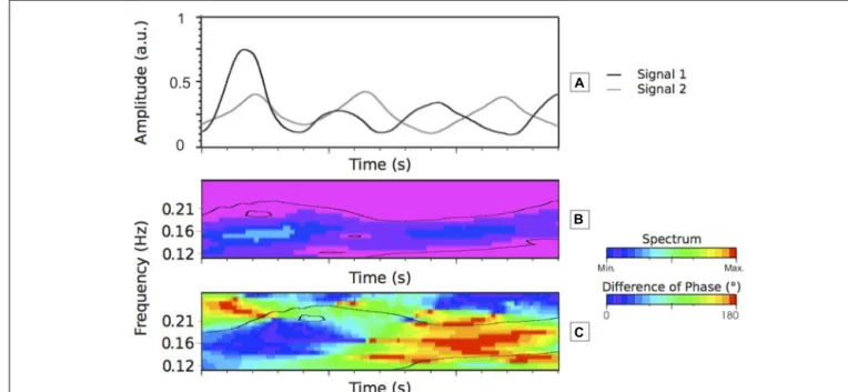
Using the CWT methods, it is possible to evaluate the prop-erties of the time-series and to estimate the individuals rating convergence and/or the divergence. Therefore the dynamic of the time-series can be compared. We can evaluate whether the raters consider that the emotional states of the participant are evolving at the same time (i.e., same speed of emotional state change). If they have the same dynamic, we will also be able to discern if the traces evolve in the same direction or not giv-ing us some information concerngiv-ing the nature of the ratgiv-ing (the RP) and its dynamic. Figure 5C represents the RP values

between the two signals (Figure 5A). For example, one can be able to extract the continuous RP at a frequency of 0.16 Hz (see first method described earlier on in the HOW section). The RP values obtained for these given signals will be ranged from 0 to 180◦ RP over the duration of the time-series. The range of colors should help the reader in understanding the RP values. This will suggest that both raters judged at the same time an expression of the emotional state, but for one of the raters the emotional state rises and for the other one it falls suggesting that although the two raters have the dame dynamic (the same frequency), they go to an opposite direction (see Figure 5C where the values go from 0◦ – the two raters are in-phase – to 180◦ – the two raters are in anti-phase). In the next section, figures and statistical analyses will illustrate how we can extract some information on such time-series using the CWT method.

To identify the significant structures from a passive or noisy component of the CWT results, theTorrence and Compo (1998)

method has been used [see HOW to Extract Useful Informa-tion from a Time-Frequency RepresentaInforma-tion (SeeFlowchart Step 4)]. As recommended by these authors, the desired level of 95% confidence has been applied.

ANALYSIS AND DISCUSSION

The analysis of the time-series was performed with the Morlet analyzing function (Steps 1 and 2 of the Flowchart). This analyzing function is polyvalent in analyzing non-stationary time-series. To

FIGURE 5 | Cross wavelet transform analysis of two males time-series (Signals 1 and 2). (A) is the representation of Signals 1 and 2. The two signals seem to have a similar dynamic (similar frequency and similar direction) at the beginning but then while keeping a similar frequency the signals tend to be move in opposite direction. (B) Shows the CWT spectrum (scalogram) of Signals 1 and 2. The black lines delineate the area statistically significant of the common frequencies of Signals 1 and 2, reflecting the local degree of interaction between the two analyzed time-series. The highest

spectrum value occurs at the beginning of (B). This is mainly explained by the high amplitude (i.e., intensity) of Signal 1. Visually one can estimate the common frequency of the two signals around a value of 0.16 Hz. (C) Shows the RP between Signals 1 and 2. (C) Confirms the visual description of (A) where for the first part of the time-series, the two signals are closed to a phase pattern drifting to an anti-phase pattern toward the end of the time-series. The range of colors facilitates the visualization of the associated RP from in-phase (close to 0◦) to anti-phase (close to 180◦). a.u., arbitrary unit.