HAL Id: hal-00298292
https://hal.archives-ouvertes.fr/hal-00298292
Submitted on 12 Oct 2006
HAL is a multi-disciplinary open access
archive for the deposit and dissemination of
sci-entific research documents, whether they are
pub-lished or not. The documents may come from
teaching and research institutions in France or
abroad, or from public or private research centers.
L’archive ouverte pluridisciplinaire HAL, est
destinée au dépôt et à la diffusion de documents
scientifiques de niveau recherche, publiés ou non,
émanant des établissements d’enseignement et de
recherche français ou étrangers, des laboratoires
publics ou privés.
height variability in the North Atlantic Ocean
D. Cromwell
To cite this version:
D. Cromwell. Temporal and spatial characteristics of sea surface height variability in the North
Atlantic Ocean. Ocean Science, European Geosciences Union, 2006, 2 (2), pp.147-159. �hal-00298292�
www.ocean-sci.net/2/147/2006/
© Author(s) 2006. This work is licensed under a Creative Commons License.
Ocean Science
Temporal and spatial characteristics of sea surface height variability
in the North Atlantic Ocean
D. Cromwell
Ocean Observing and Climate, National Oceanography Centre, Southampton (NOCS), Room 254/35, European Way, Southampton SO14 3ZH, UK
Received: 29 March 2006 – Published in Ocean Sci. Discuss.: 21 June 2006
Revised: 8 September 2006 – Accepted: 5 October 2006 – Published: 12 October 2006
Abstract. We investigate the spatial and temporal variability of sea surface height (SSH) in the North Atlantic basin us-ing satellite altimeter data from October 1992–January 2004. Our primary aim is to provide a detailed description of such variability, including that associated with propagating sig-nals. We also investigate possible correlations between SSH variability and atmospheric pressure changes as represented by climate indices.
We first investigate interannual SSH variations by deriv-ing the complex empirical orthogonal functions (CEOFs) of altimeter data lowpass-filtered at 18 months. We determine the spatial structure of the leading four modes (both in am-plitude and phase) and also the associated principal compo-nent (PC) time series. Using wavelet analysis we derive the time-varying spectral density of the PCs, revealing when par-ticular modes were strongest between 1992–2004. The spa-tial pattern of the leading CEOF, comprising 30% of the to-tal variability, displays a 5-year periodicity in phase; signal propagation is particularly marked in the Labrador Sea. The second mode, with a dominant 3-year signal, has strong vari-ability in the eastern basin.
Secondly, we focus on the Azores subtropical frontal zone. The leading mode (35%) is strong in the south and east of this region with strong variations at 3- and 5-year periods. The second mode (21%) has a near-zonal band of low vari-ance between ∼22◦–27◦N, sandwiched between two regions of high variance. Thirdly, we lowpass filter the altimeter data at a cutoff of 30 days, instead of 18 months, in order to retain signals associated with propagating baroclinic Rossby waves and/or eddies. The leading mode is the annual steric sig-nal, around 46% of the SSH variability. The third and fourth CEOFs, ∼11% of the remaining variability, are associated with westward propagation which is particularly dominant in a “waveband” between 32◦–36◦N.
Correspondence to: D. Cromwell ([email protected])
For all three cases considered above, no significant cross-correlation is found between the North Atlantic Oscillation index and the amplitude of the leading four PCs of in-terannual SSH variability. The only exception is an anti-correlation found over the North Atlantic basin between the NAO and the 4th PC. In the subtropical front, the East At-lantic Pattern index is anti-correlated with the leading PC for SSH variations lowpass filtered at 30 days. Further investi-gation of forcing mechanisms is suggested using hindcasts from ocean general circulation models.
1 Introduction
The ocean circulation and dynamics of the North Atlantic Ocean play an important role in the climate system. In partic-ular, the significance of the thermohaline circulation “global conveyor belt”, which carries warm water north towards the poles and returns cold water at depth, is well known (Broecker, 1991). Much recent interest has focused on the meridional overturning circulation (Schiermeier, 2006) and, in particular, on the finding that the MOC at 25◦N has appar-ently slowed by around 30% (Bryden, 2005).
Levermann et al. (2005) suggest on the basis of modelling studies that a weakening of the thermohaline circulation could generate dynamic sea surface height (SSH) changes that locally reach up to ∼1 m. According to H¨akkinen and Rhines (2004), in the last two decades there has been an in-crease in SSH in the North Atlantic subpolar gyre and a re-duction in the strength of the North Atlantic subpolar gyre in the 1990s. However, they stressed that because of the lack of SSH data prior to 1978, there is uncertainty as to whether or not this feature is a decadal cycle or a long-term trend.
Although this study does not tackle these issues directly, our aim is to provide an improved quantitative description of spatio-temporal SSH variability in the North Atlantic, a nec-essary step towards being able to detect unambiguously any
long-term trends. Moreover, we aim to provide an improved description of SSH variability associated with propagating signals: an important means by which one part of the ocean-atmosphere system communicates with another (Gill, 1982; Jacobs et al., 1994).
The paper is structured as follows. In Sect. 2.1 we de-scribe the data. We apply two well-established methods in geophysical signal processing: complex empirical orthog-onal function decomposition and wavelet analysis. CEOF analysis (Sect. 2.2) yields information on the observed spa-tial and temporal variability in SSH, particularly where prop-agating features, such as baroclinic Rossby waves and ed-dies, are known to contribute to variability. Wavelet analysis (Sect. 2.3) reveals the time-varying spectral content of SSH signatures. We present our results in Sect. 3. In Sect. 3.1 we investigate the interannual SSH variability in the North At-lantic Ocean. In Sect. 3.2 we focus on the dynamic region around the Azores subtropical front. Here we investigate both interannual variability as well as subannual variability associated with propagating baroclinic features. In Sect. 3.3, we investigate possible links between the observed SSH vari-ability and two leading modes of atmospheric varivari-ability rep-resented by the North Atlantic Oscillation and East Atlantic Pattern climate indices. Finally we summarise and discuss the results in Sect. 4.
2 Data and methodology
2.1 Data description
We use the merged altimeter data product known as DU-ACS (Developing Use Of Altimetry For Climate Stud-ies) which incorporates altimeter data from the ERS and TOPEX/Poseidon satellites and their successors, respec-tively, Envisat and Jason. The DUACS dataset was produced by the CLS Space Oceanography Division and AVISO, the French space agency. The data are sea surface height anoma-lies on a Mercator spatial grid of (1/3)◦ longitude × (1/3)◦ cos(latitude). The temporal sampling of the data is 7 days, and the period covered is October 1992–January 2004.
Details of the data processing and mapping method can be found in Le Traon and Ogor (1998) and Le Traon et al. (1998). Standard corrections are applied including the inverse barometer correction. The reader is also referred to the DUACS handbook, http://www.jason.oceanobs.com/ documents/donnees/duacs/handbook duacs.pdf, and to CLS (2004) for further details.
2.2 Complex empirical orthogonal function analysis Empirical orthogonal function (EOF) analysis allows one to decompose a dataset in terms of its statistical modes of vari-ability. These modes are obtained by performing an eigen-value analysis of the covariance matrix of the data. This yields eigenvectors, which can be mapped as spatial patterns
of variability, and associated principal components (PCs), each of which describes the time evolution of the correspond-ing spatial structure.
In complex EOF analysis we first “complexify” the data. Thus, if Xt is the original real time series that we are in-terested in (SSH variations, for example), then we gener-ate a relgener-ated time series: Xt⇒Xt+iXtH where XtH is the Hilbert transform of the original data (von Storch and Zwiers, 1999). We can then apply conventional eigentechniques such as EOFs to the complexified time series. This yields statis-tical patterns that contain both real and imaginary compo-nents. It is more physically meaningful to represent the data decomposition in terms of amplitude and phase. This treat-ment also naturally lends itself to examination of any propa-gating features in the original data; determining propagation in SSH variations is an important focus of the present study. Moreover, as Fu (2004) notes, the complex EOF approach is more efficient than a regular EOF analysis because of the importance of capturing the phase information in the SSH variability.
The convention adopted in this study is that progression in time corresponds to anti-clockwise rotation of the eigenvec-tor phase. Note that, because zero phase angle is an arbitrary choice, the direction of a phase arrow at any particular geo-graphical location is unimportant. What matters is whether, and in what sense, the direction of the phase arrow changes between one location and another. Thus, if a spatial region of high-amplitude SSH signal has the phase arrows rotating anti-clockwise from east to west, this indicates a strong west-ward propagating signal. Tourre et al. (1998) used complex EOFs in their study of interdecadal variation and propagat-ing features in the Pacific Ocean (but note that they used the opposite sign convention for rotation of phase arrows and di-rection of propagation).
To summarise: complex EOF analysis yields for each sta-tistical mode a map of the complex-valued spatial variability pattern (i.e. both amplitude and phase) as well as an associ-ated complex principal component (PC) which can be plotted as a time series of amplitude and phase. Anticlockwise ro-tation of the phase arrow between one spatial location and another indicates signal progression in time. As we see in the following section, a wavelet analysis of the PC can be performed thereafter to yield the time-varying spectral con-tent of the associated complex EOF mode.
2.3 Wavelet analysis
The wavelet method allows one to analyse localised power variations within a discrete series at a range of scales (Foufoula-Georgiou and Kumar, 1994). Wavelets can be considered as building blocks in a decomposition or se-ries expansion using dilated and translated versions of a mother wavelet each multiplied by an appropriate coeffi-cient (Farge, 1992). The local wavelet power spectrum is the square of the wavelet coefficients (Torrence and Compo,
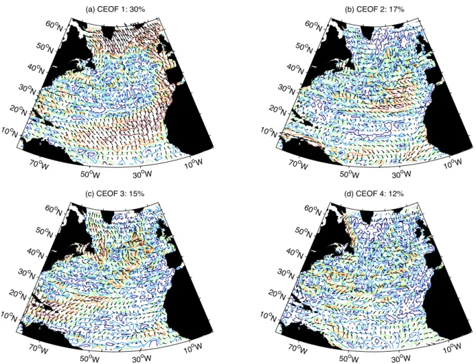
(a) CEOF 1: 30% 70o W 50oW 30oW 10oW 10o N 20o N 30o N 40o N 50o N 60o N (b) CEOF 2: 17% 70o W 50oW 30oW 10oW 10o N 20o N 30o N 40o N 50o N 60o N (c) CEOF 3: 15% 70o W 50oW 30oW 10 oW 10o N 20o N 30o N 40o N 50o N 60o N (d) CEOF 4: 12% 70o W 50oW 30oW 10 oW 10o N 20o N 30o N 40o N 50o N 60o N
Fig. 1. Results of a complex empirical orthogonal function (CEOF) analysis of DUACS altimeter sea surface height anomaly measurements
in the North Atlantic basin (10◦–65◦N, 80◦–0◦W) for the period October 1992–January 2004. The input data are on a regular 1◦×1◦grid, have a sampling period of 1 week and have been lowpass-filtered to remove periods shorter than 18 months. Subplots (a)–(d): Maps of first four CEOF modes with amplitude contours (in arbitrary units; five contours with regular intervals from minimum to maximum) and phase overlaid as arrows (anticlockwise rotation of phase arrows from one location of strong amplitude to another indicates propagating signal). The title of each subplot gives the mode number and its percentage contribution to the total variability.
1998). The global wavelet spectrum is the average spec-trum over all time, equivalent to the Fourier specspec-trum. We make the usual choice here of adopting the Morlet wavelet, a complex-valued, modulated Gaussian plane wave widely used in the study of geophysical processes. It is described by
ψ (η)=π−1/4eiωηe−η2/2, where ω is the nondimensional fre-quency which must be equal to, or greater than, 5 to satisfy the wavelet admissibility condition (Farge, 1992). To sup-press edge effects and to speed up computation, zero padding to the next higher power of two is performed prior to the wavelet transformation. The cone of influence is that part of the wavelet spectrum, at longer periods, in which edge effects become important. It is defined as the e-folding time for the autocorrelation of wavelet power at each scale (Torrence and Compo, 1998).
3 Results of data analysis
3.1 Interannual sea surface height variability in the North Atlantic Ocean
We focus first on the interannual sea surface height variabil-ity in the North Atlantic Ocean region spanning 10◦–65◦N, 80◦–0◦W. The data are lowpass filtered to remove variability with periods shorter than 18 months. The data are then re-gridded to 1◦×1◦(retaining the original high-resolution DU-ACS gridding exceeded the available computing capacity to perform CEOF analysis for the whole region). Our initial approach has similarities to that of Fu (2004) who studied interannual SSH variation in the North Atlantic; however we take it further in several respects. First, we extend the anal-ysis in that we investigate not just the leading CEOF mode but the first four modes giving a more complete description
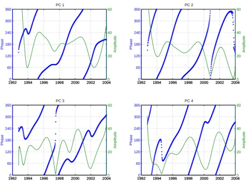
19920 1994 1996 1998 2000 2002 2004 60 120 180 240 300 360 Phase PC 1 1992 1994 1996 1998 2000 2002 20040 20 40 60 Amplitude 19920 1994 1996 1998 2000 2002 2004 60 120 180 240 300 360 Phase PC 2 1992 1994 1996 1998 2000 2002 20040 20 40 60 Amplitude 19920 1994 1996 1998 2000 2002 2004 60 120 180 240 300 360 Phase PC 3 1992 1994 1996 1998 2000 2002 20040 20 40 60 Amplitude 19920 1994 1996 1998 2000 2002 2004 60 120 180 240 300 360 Phase PC 4 1992 1994 1996 1998 2000 2002 20040 20 40 60 Amplitude Figure 2
Fig. 2. Principal component time series corresponding to the maps of CEOF modes plotted in Fig. 1 (North Atlantic SSH anomalies, 1◦×1◦
gridding, lowpass-filtered at 18 months). Both phase (in degrees; blue) and amplitude (arbitrary units; green) are shown.
of SSH variability. This is further enhanced by applying wavelet analysis to determine the time-varying spectral con-tent of the principal components. Moreover, in the next sec-tion, we home in on the dynamic Azores subtropical frontal region of the northeast Atlantic. Note that in this particular region we apply filtering that retains the baroclinic Rossby wave and/or eddy signal, unlike Fu (2004).
First, consider the results of the CEOF analysis for the whole North Atlantic basin. In Fig. 1, we plot the spatial patterns of the leading four CEOFs. Recall that the modes are complex-valued; we plot both the spatial CEOF ampli-tude (coloured contours) and phase (arrows). In Fig. 2, we plot the complex-valued time series of the associated prin-cipal components: amplitude (green line) and phase (blue circles) are plotted for each. The leading CEOF mode repre-sents 30% of the total SSH variability and the sum of the first four modes accounts for 74%. We use the Lambert conical projection for the maps as it takes account of the latitudinal variation in length (in km) of a fixed span of degrees longi-tude.
3.1.1 Complex EOF Mode 1
It can be seen from Fig. 2 that the phase time series of PC1 (the principal component of the leading CEOF mode) has a dominant period of ∼5–6 years. The corresponding am-plitude map in Fig. 1 has a tripole-like structure: two do-mains of high SSH variability in the subpolar gyre and at low latitudes with a region of low variability between them. The two high variability regions at high and low latitudes are linked by a ridge of high variability along the eastern
bound-ary. There is no consistent rotation of the phase arrows along this ridge and thus no unambiguous evidence of actual signal propagation here.
It is known that there is a sea surface temperature tripole associated with the North Atlantic Oscillation (Marshall et al., 2001). There is a degree of similarity between the pat-terns in SST and the leading-mode SSH, though the former does not display the high-variability ridge along the east-ern boundary. Interestingly, Pingree (2002) observed SSH anomalies from altimetry between 1992 and 2002 and found that the eastern SSH boundary off west Europe was tilted strongly in January 1996 and November/December 1997. This may at least partly explain the eastern boundary struc-ture observed in Fig. 1a. Note that there is evidence of SSH propagation in the northwest Atlantic and Labrador Sea: a clear anticlockwise rotation of phase arrows moving north and west from Newfoundland towards the west of Greenland. Wavelet analysis of both the phase and amplitude time se-ries components of PC1 were carried out (plots not included). This confirmed a ∼5 year cycle in phase propagation and showed a peak in strength around 1998. The dominant cy-cle in the amplitude component of PC1 has a period of ∼3–4 years and has peaks in 1994 and 2002. Note that the strength of a mode, as indicated by its amplitude, does not neces-sarily coincide with times when any propagation, revealed by pronounced phase changes, associated with that mode is strongest. In other words, forcing may drive strong SSH vari-ability but not necessarily a strongly propagating signal.
3.1.2 Complex EOF Mode 2
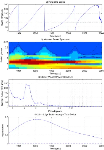
The spatial pattern of the second CEOF (17% of the total variability) has a different structure from the leading CEOF. The regions of high variability are concentrated in the east-ern subtropical gyre between ∼30◦–40◦N, and in the trop-ics (∼5◦–15◦N), particularly west of 50◦W. As we see from Fig. 2, the phase time series of PC2 has a cycle of ∼3 years. We analysed the time-varying spectral energy of this time se-ries by subjecting it to a wavelet analysis, the results of which are shown in Fig. 3. From top to bottom, we see: (a) the in-put time series (i.e. the phase of PC2); (b) the wavelet power spectrum of (a), where the dashed line indicates the cone of influence below which (i.e. at longer periods) edge effects become important given the finite length of the time series (Torrence and Compo, 1998); (c) the global wavelet power spectrum, i.e. time integral of (b); (d) time series of the scale average of wavelet power spectrum in the period range 2.5– 3.5 years (to capture the dominant cycle of ∼3 years).
In the case of CEOF mode 2, the amplitude time series of PC2, like the phase component, has a dominant timescale of ∼3 years. Strong phase propagation is observed around 1996.
3.1.3 Complex EOF Mode 3
Mode 3 comprises 15% of the total variability. The general spatial pattern is of high amplitude variability in the western tropics, Gulf Stream extension, Labrador Sea and around the Mid-Atlantic Ridge north of ∼35◦N. Wavelet analysis re-veals a strong ∼2-year cycle in both phase and amplitude. The phase signal peaks in 1996 and is weak after 2001, whereas the amplitude of the 2-year signal starts low and peaks in around 2001. There is also a 4-year cycle in am-plitude, peaking around 2000.
3.1.4 Complex EOF Mode 4
Mode 4 represents 12% of the total variability and comprises isolated patches as well as ridges of SSH variability, notably in the western Labrador Sea. Wavelet analysis of PC4 re-veals 3.5-year cycles in phase and amplitude with peaks in both around 2000. There is also a 5-year cycle in amplitude, peaking around 1998.
In Table 1, we summarise the characteristics of all four leading modes for the 18-month lowpass filtered data in the North Atlantic Ocean. It is worth noting that Pingree (2005) also observed multi-year cycles in SSH variability (though this was not a complex EOF analysis and did not yield in-formation on signal propagation): a 2-year signal in the Gulf Stream region, a 4-year periodicity in parts of the subtropi-cal gyre, and an 8-year cycle in the Gulf Stream region and linked to subpolar regions. This 8-year cycle appears to have a “pivot” or node (region of minimum SSH amplitude) near
Fig. 3. Wavelet analysis of the principal component phase
associ-ated with the second CEOF in sea surface height anomaly in the North Atlantic (PC2 in Fig. 2). (a) Input time series, i.e. the phase of PC2; (b) wavelet power spectrum of (a); (c) global wavelet power spectrum, i.e. integral of (b) over time; (d) time series of scale av-erage of (b) in period range 2.5–3.5 years. In (b), the dashed line indicates the cone of influence, below which edge effects become important, and the solid contour is the 95% confidence level (or, equivalently, the 5% significance level). In (c) and (d), the 95% confidence level is indicated by a dashed line.
the latitude of the RAPID programme’s MOC monitoring ar-ray at 26◦N (Schiermeier, 2004).
3.2 Sea surface height variability in the Azores subtropical front
3.2.1 Interannual variability: lowpass filtering at 18 months We now focus on the northeast Atlantic (20◦–40◦N, 50◦– 10◦W), encompassing the Azores subtropical front (Gould, 1985). This region is rich in westward propagating Rossby waves and eddies (Tokmakian and Challenor, 1993; Cipollini et al., 1997, 1998; Pingree, 1997, 2002; Tychensky et al., 1998). Given the smaller geographical domain, we now have sufficient computing capacity to calculate CEOFs for the
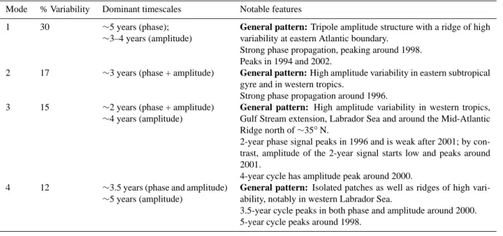
Table 1. Summary of the characteristics of the leading four complex EOF modes of DUACS altimeter sea surface height anomaly
measure-ments in the North Atlantic basin (10◦–65◦N, 80◦–0◦W) for the period October 1992–January 2004. The input data are on a regular 1◦×1◦ grid, have a sampling period of 1 week and have been lowpass-filtered to remove periods shorter than 18 months. Thus, the focus here is on interannual variability.
Mode % Variability Dominant timescales Notable features
1 30 ∼5 years (phase);
∼3–4 years (amplitude)
General pattern: Tripole amplitude structure with a ridge of high
variability at eastern Atlantic boundary. Strong phase propagation, peaking around 1998. Peaks in 1994 and 2002.
2 17 ∼3 years (phase + amplitude) General pattern: High amplitude variability in eastern subtropical
gyre and in western tropics.
Strong phase propagation around 1996.
3 15 ∼2 years (phase + amplitude)
∼4 years (amplitude)
General pattern: High amplitude variability in western tropics,
Gulf Stream extension, Labrador Sea and around the Mid-Atlantic Ridge north of ∼35◦N.
2-year phase signal peaks in 1996 and is weak after 2001; by con-trast, amplitude of the 2-year signal starts low and peaks around 2001.
4-year cycle has amplitude peak around 2000.
4 12 ∼3.5 years (phase and amplitude)
∼5 years (amplitude)
General pattern: Isolated patches as well as ridges of high
vari-ability, notably in western Labrador Sea.
3.5-year cycle peaks in both phase and amplitude around 2000. 5-year cycle peaks around 1998.
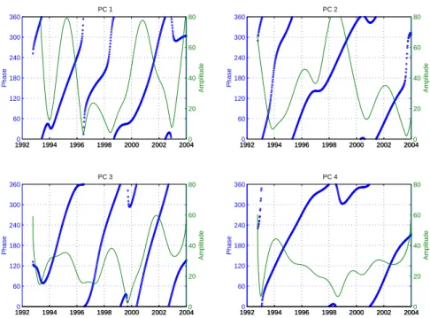
DUACS dataset at its original high-resolution spatial grid-ding of (1/3)◦longitude × (1/3)◦cos(latitude). Figures 4 and 5, analogous to Figs. 1 and 2, respectively, show the results of the complex EOF analysis: amplitude and phase maps of the leading four CEOFs and the associated principal compo-nents. These four modes account for 79% of the total vari-ability.
Note that wavelet analysis of a phase time series captures quantitatively the periodicity, or multiple periodicities, of a signal: when the phase associated with a propagating fea-ture moves through 0 to 360◦ then back to 0 before rising once again to 360◦, wavelet analysis tracks this phase evo-lution with time. Caution is required, however; there are a small number of occurrences where a slight change in phase angle causes a spurious jump between 360 to 0 and back to 360. For example, in Fig. 5, the plot of PC2 shows such be-haviour between 2000–2001. However, care has been taken in the interpretation to exclude such spurious events from the mode descriptions provided in the main text and in the tables. Note, too, that although visual inspection of the time between nodes of the time series plot of phase can give a first approx-imation of the dominant period, this is not always possible; in particular, where more than one strong period is present in the signal. Hence, wavelet analysis is a valuable tool in the data analysis and interpretation.
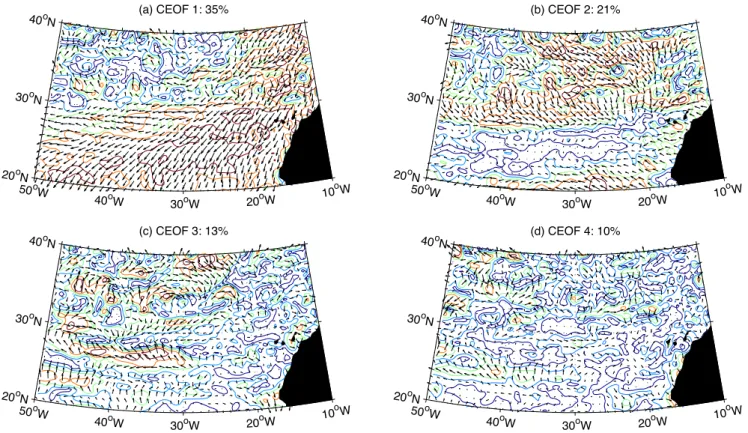
(a) Complex EOF Mode 1
As shown in Fig. 4, the leading mode (35% of the to-tal variability) is strong in the south and east, consistent with the pattern found in Sect. 3.1 (North Atlantic basin). In particular, there is strong variability south of 30◦N and also everywhere east of ∼25◦W, with one order of magnitude lower variability elsewhere.
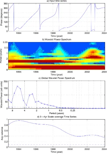
Figure 6 shows the wavelet analysis of the phase of the leading mode displaying strong propagation at ∼3 years and
∼5 years (though the latter must be treated with caution in this smaller geographical domain because it falls beneath the cone of influence). The scale-averaged energy of the phase component of PC1 in the period range 2–4 years (thus capturing the ∼3-year signal) decays gradually from a peak in 1994. Wavelet analysis of the amplitude component of PC1 reveals peaks in 1994 and 2002, with a low at the midpoint in 1998. There is also a 5-year cycle in phase (but not amplitude), peaking around 1998. Again, because of the limited length of the time series, this result must be treated with caution.
(b) Complex EOF Mode 2
The second mode (21% of the total variability) has a different spatial distribution: a near-zonal band of lower variance at ∼22◦–27◦N, sandwiched between two regions of higher variance. Again, the levels of variance across the subtropical region span around one order of magnitude.
(a) CEOF 1: 35% 50o W 40o W 30o W 20oW 10 oW 20o N 30o N 40o N (b) CEOF 2: 21% 50o W 40o W 30o W 20oW 10 oW 20o N 30o N 40o N (c) CEOF 3: 13% 50o W 40o W 30o W 20oW 10 oW 20o N 30o N 40o N (d) CEOF 4: 10% 50o W 40o W 30o W 20oW 10 oW 20o N 30o N 40o N
Fig. 4. Results of a complex empirical orthogonal function (CEOF) analysis of DUACS altimeter sea surface height anomaly measurements
in the northeast Atlantic basin (20◦–40◦N, 50◦–10◦W) for the period October 1992–January 2004. The input data are on a Mercator (1/3)◦ longitude × (1/3)◦cos(latitude) latitude grid, have a sampling period of 1 week and have been lowpass-filtered to remove periods shorter than 18 months. Subplots (a)–(d): Maps of first four CEOF modes with amplitude contours (in arbitrary units; five contours with regular intervals from minimum to maximum) and phase overlaid as arrows (anticlockwise rotation of phase arrows from one location of strong amplitude to another indicates propagating signal).
Wavelet analysis reveals strong phase propagation with a period of 2 years, peaking in 1995 with a secondary peak in 2001. A 3-year amplitude signal is also found, peaking around 2000. Finally, and again with caution, a 5-year phase signal is seen, also peaking around 2000.
(c) Complex EOF Mode 3
Mode 3 carries 13% of the total variability. Its spatial structure comprises ridges and local patches of high SSH variability, including a near-zonal band at 28◦N. A dominant 3-year cycle is observed in both phase and amplitude. Peaks are seen in 1997 (phase) and 1999 (amplitude).
(d) Complex EOF Mode 4
This mode has around 10% of the total variability. Its general pattern reveals a few local patches of moderate variability, mostly west of 35◦W. A 3-year amplitude signal is seen in the wavelet analysis, peaking in 1994. There is also a 4-year cycle in phase showing strongest signal propagation between 1998–2002.
The characteristics of all four leading modes for the 18-month lowpass filtered data in the region of the Azores sub-tropical front are summarised in Table 2.
3.2.2 Subannual baroclinic propagation: lowpass filtering at 30 days
As mentioned above, it is well known that westward propa-gating baroclinic Rossby waves and/or eddies can be seen in SSH observations in the mid-latitudes of the North Atlantic basin. In particular, a “waveband” of enhanced SSH variabil-ity associated with such features is concentrated in a quasi-zonal strip centred near 34◦N (Cromwell, 2001). The peri-odicity is known to be subannual (∼6–10 months); lowpass filtering at 18 months would remove them. To study these signals, we therefore lowpass filter the data with a cutoff of 30 days, rather than 18 months, thus retaining the baroclinic SSH signal but removing higher-frequency variability. We then perform CEOF analysis followed by wavelet analysis of the principal components, just as before.
19920 1994 1996 1998 2000 2002 2004 60 120 180 240 300 360 Phase PC 1 1992 1994 1996 1998 2000 2002 20040 20 40 60 80 Amplitude 19920 1994 1996 1998 2000 2002 2004 60 120 180 240 300 360 Phase PC 2 1992 1994 1996 1998 2000 2002 20040 20 40 60 80 Amplitude 19920 1994 1996 1998 2000 2002 2004 60 120 180 240 300 360 Phase PC 3 1992 1994 1996 1998 2000 2002 20040 20 40 60 80 Amplitude 19920 1994 1996 1998 2000 2002 2004 60 120 180 240 300 360 Phase PC 4 1992 1994 1996 1998 2000 2002 20040 20 40 60 80 Amplitude Figure 5
Fig. 5. Principal component time series corresponding to the maps of CEOF modes plotted in Fig. 4 (northeast Atlantic SSH anomalies,
(1/3)◦×(1/3)◦cos(latitude) grid, lowpass-filtered at 18 months). Both phase (in degrees; blue) and amplitude (arbitrary units; green) are shown.
(a) Complex EOF Mode 1
The leading mode is the annual steric signal which ac-counts for 46% of the total SSH variability.
(b) Complex EOF Mode 2
Mode 2 comprises 5% of the total variability; if the annual steric cycle is discounted, the second mode has 10% of the remaining variability. The general spatial pattern displays strongest variability in the region ∼35◦–25◦W, 32◦–40◦N. A number of dominant timescales in phase and/or amplitude are seen. A 5-year cycle in phase is cautiously identified, peaking around 1999. A cycle of ∼3 years in amplitude is visible, with a peak around 1997. There is also a ∼1.5 year signal in phase, with significant phase propagation observed between 1993–1997. A ∼1-year cycle in amplitude is observed between 2000–2002. Finally, a
∼6-month signal of phase propagation is observed between 2001–2003.
(c) Complex EOF Mode 3
The third mode has 2.9% of the total variability (5.4% of non-steric variability). Figure 7 shows the spatial pattern of mode 3. Note the concentration of SSH variability in a near zonal band at 32◦–36◦N. Note, too, the anticlockwise rotation of the phase vector from east to west, consistent with westward propagation in this region. The hand-plotted
trajectory of propagation has been determined via close visual inspection of the geographical locations of amplitude peaks around which the phase arrows rotate. We have thus found for the first time, as far as we are aware, the variation in the trajectory (in both longitude and latitude) of the propagation of Rossby waves and/or eddies in this region. By estimating the period (∼230 days) of this mode from the associated principal component (not plotted here), and the spatial distance over which a 360◦rotation of the phase arrow occurs, yielding a wavelength of ∼520 km, we can estimate the speed of the Rossby waves at this latitude as
∼2.7 cm/s. This confirms earlier estimates from satellite altimeter observations (Chelton and Schlax, 1996; Cipollini et al., 1997). Although sporadic in situ observations provide depth-dependent mesoscale ocean structure, and can thus help distinguish between waves and eddies, Pingree and Sinha (2001) and Pingree (2002) have noted that eddies in the zonal waveband studied here have wavelike properties. It is therefore difficult to determine whether periodic Rossby waves or quasi-regular pulses of mesoscale eddies are being observed, particularly using satellite observations alone.
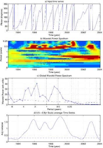
We then perform a wavelet analysis of the phase com-ponent of PC3, yielding detailed information about the phase propagation corresponding to baroclinic features (Fig. 8). Figure 8b shows strong spectral content at the subannual periods characteristic of Rossby waves at mid-latitudes. There is also strong variability at periods of 2–4 years, though after 2001 this energy lies below the cone of influence (dashed line) and must be treated with caution
Fig. 6. Wavelet analysis of the principal component phase
associ-ated with the leading CEOF in sea surface height anomaly over the northeast Atlantic (PC1 of Fig. 5). The dataset has been lowpass-filtered to remove signals shorter than 18 months. (a) Input time series, i.e. the phase of PC1; (b) wavelet power spectrum of (a); (c) global wavelet power spectrum, i.e. integral of (b) over time; (d) time series of scale average of (b) for periods in range 2–4 years. In (b), the dashed line indicates the cone of influence, below which edge effects become important, and the solid contour is the 95% confidence level. In (c) and (d), the 95% confidence level is indi-cated by a dashed line.
because of the usual edge effects. The global wavelet plot in Fig. 8c shows several strong peaks at around 8 months, 2 years and 3.3 years. Thus, the phase time series plotted in 8a has a number of dominant periods: a clear example where mere visual inspection of the time between nodes will not lead to a reliable single value for the dominant period, therefore showing once again the value of wavelet analysis. In Fig. 8d, scale-averaging over the period range of 0.5–0.8 years (∼6–10 months) reveals the time-varying strength of the Rossby wave signal. There are peaks in 1996, 1997, 1999 and again in 2003. These are likely related to peaks in forcing mechanism(s). 50oW 30oW 10oW 20oN 30oN 40oN Figure 7
Fig. 7. Spatial pattern of 3rd CEOF of sea surface height anomaly in
northeast Atlantic after lowpass-filtering at 30 days. Both amplitude (coloured contours; arbitrary units) and phase (arrows) are shown. Phase rotation in the zonal band ∼32◦–36◦N west of ∼30◦W is characteristic of the westward propagation of baroclinic Rossby waves in this region. The solid black line indicates the observed trajectory of the Rossby waves. This has been determined via close visual inspection of the geographical locations of amplitude peaks around which the phase arrows rotate.
(d) Complex EOF Mode 4
CEOF mode 4 has 2.8% of the total variability (5.2% of non-steric variability) and displays similar characteristics as mode 3 including the westward propagation (although not as clearly delineated; propagation is clearly stronger in mode 3). This indicates that the baroclinic Rossby wave energy is partitioned into both these modes with a combined variability of 11% of the non-steric SSH signal. The percentage variability associated with the Rossby waves would, of course, be greater if the domain of analysis was further restricted to the “waveband” latitude range 32◦–36◦N where the westward propagation is concentrated. The characteristics of all four leading modes for the 30-day lowpass filtered data in the region of the Azores subtropical front are summarised in Table 3.
As we noted earlier (Sect. 2.3), caution needs to be ap-plied in the interpretation of signals inside the cone of in-fluence, the region of the wavelet spectrum where edge ef-fects impact on the larger scales. In the present case of a 12– year time series, a 5-year cycle may appear marginal. How-ever, note that when the global wavelet spectrum is calculated (e.g. Fig. 3c), a signal may indeed shown to be significant at the 5% level (i.e. 95% confidence level). Likewise, the plots of scale-averaged (roughly equivalent to bandpass-filtered) time series (e.g. Fig. 3d) may show statistically significant variations. Moreover, on occasion the time-evolution of sig-nals with particular periods does appear above the cone of influence, or close to it, so that a reasonable interpretation can be made on that basis. This is particularly so when con-firmed by the presence of strong peaks in the global wavelet
Fig. 8. Wavelet analysis of the principal component phase
asso-ciated with the 3rd CEOF in sea surface height over the northeast Atlantic. The dataset has been lowpass-filtered to remove signals longer than 30 days, thus retaining subannual variability. (a) In-put time series, i.e. the phase of the 3rd principal component; (b) wavelet power spectrum of (a); (c) global wavelet power spectrum, i.e. integral of (b) over time; (d) time series of scale average of (b) for periods in range 0.5–0.8 years (∼6–10 months), corresponding to baroclinic Rossby waves at this latitude. In (b), the dashed line indicates the cone of influence, below which edge effects become important, and the solid contour is the 95% confidence level. In (c) and (d), the 95% confidence level is indicated by a dashed line.
plot and/or scale-averaged plot. It is careful interpretation of a combination of all these plots that underpins the mode descriptions in this paper, collated in Tables 1–3.
3.3 Relationship of the North Atlantic Oscillation (NAO) and East Atlantic Pattern (EAP) to sea surface height variability
Atmospheric pressure variations play a role in forcing sea surface height variability. In what follows, we take air pres-sure indices as proxies for the wind forcing. Thus, to in-vestigate a possible physical relationship between important modes of atmospheric variability and SSH variability, we
use climate indices provided by the National Oceanic and Atmospheric Administration/National Weather Service Cli-mate Prediction Center (CPC). The two leading atmospheric pressure modes in winter are the North Atlantic Oscillation (NAO) and East Atlantic Pattern (EAP). The CPC indices are available from http://www.cpc.ncep.noaa.gov/ and are de-rived from an analysis based on the work of Barnston and Livezey (1987).
We consider interannual SSH variations in (a) the North Atlantic (i.e. the work of Sect. 3.1); (b) the Azores Subtropi-cal Front: interannual variability (Sect. 3.2.1); and (c) Azores Subtropical Front: subannual variability (Sect. 3.2.2). As a measure of the strength of a mode of SSH variability, we use the amplitude of the corresponding principal component. For all three cases (a), (b) and (c) we calculate the cross-correlation coefficient (r) between each climate index (NAO and EAP) and the strength of each of the four leading com-plex EOFs. The significance of the calculated values of r takes account of the effective degrees of freedom based on the coherence and autocorrelation of the data (Emery and Thomson, 1997). Table 4 summarises the results.
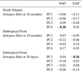
For all three cases considered, no significant cross-correlation is found between both the NAO or EAP index and the amplitude of the leading four PCs of interannual SSH variability. There are two exceptions, both involving correlations: (1) in the North Atlantic basin, there is an anti-correlation (r=−0.26) between the NAO and PC4; (2) in the subtropical front, the EAP index is anti-correlated (r=−0.36) with the leading PC for SSH variations lowpass-filtered at 30 days. We discuss this further in the concluding section.
The small values of r indicate that, although the relevant mode of atmospheric pressure variability plays a significant role in explaining the corresponding mode of SSH variance, it cannot be the dominating factor (since r2<0.5). Exten-sive modelling studies, beyond the scope of this study, would be required to investigate the relative role of possible forc-ing mechanisms such as baroclinic instability, bursts in wind stress or seasonal variations in local currents.
4 Discussion and conclusions
We have investigated the variability of sea surface height in the North Atlantic basin using a merged DUACS satel-lite altimeter dataset spanning October 1992–January 2004. By applying complex empirical orthogonal function analy-sis we determined the spatial and temporal structure of SSH variability, including evidence of propagating features, for the leading four modes. Using wavelet analysis we deter-mined the time-varying spectral density content of the prin-cipal components.
We first investigated the interannual variability in the North Atlantic by lowpass filtering the SSH data at a cut-off of 18 months. The spatial pattern of the leading com-plex EOF, comprising 30% of the total variability, showed
Table 2. Summary of the characteristics of the leading four complex EOF modes of DUACS altimeter sea surface height anomaly
measure-ments in the northeast Atlantic (20◦–40◦N, 50◦–10◦W) for the period October 1992–January 2004. The input data are on a high-resolution Mercator grid of (1/3)◦in longitude × (1/3)◦cos(latitude) in latitude, have a sampling period of 1 week and have been lowpass-filtered to remove periods shorter than 18 months. Thus, the focus here is on interannual variability.
Mode % Variability Dominant timescales Notable features
1 35 ∼3 years (phase + amplitude)
∼5 years (phase)
General pattern: Strong variability south of 30◦N and also
ev-erywhere east of ∼25◦W; one order of magnitude lower variability elsewhere.
Amplitude of 3-year cycle peaks in 1994 and 2002, with a low in 1998. Phase of 3-year cycle strongest in 1994.
5-year phase cycle peaks around 1998.
2 21 ∼2 years (phase)
∼3 years (amplitude) ∼5 years (phase)
General pattern: Near-zonal band of low variance at ∼22◦–27◦N
sandwiched between two regions of higher variance. Again, the levels of variance span around one order of magnitude.
Phase propagation with period of 2 years peaks in 1995, with a secondary peak in 2001.
3-year amplitude signal peaks around 2000. 5-year phase signal peaks around 2000.
3 13 ∼3 years (phase + amplitude) General pattern: Ridges and local patches of high variability,
in-cluding near-zonal band at 28◦N.
Peaks in 1997 (phase) and 1999 (amplitude).
4 10 ∼3 years (amplitude)
∼4 years (phase)
General pattern: A few local patches of moderate variability,
mostly west of 35◦W.
3-year amplitude signal peaks in 1994.
Strongest 4-year phase propagation between 1998–2002.
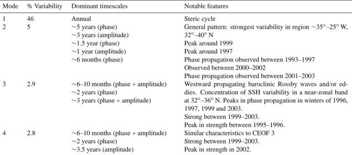
Table 3. Summary of the characteristics of the leading four complex EOF modes of DUACS altimeter sea surface height anomaly
measure-ments in the Azores Subtropical Front region (20◦–40◦N, 50◦–10◦W) for the period October 1992–January 2004. The input data are on a high-resolution Mercator grid of (1/3)◦in longitude × (1/3)◦cos(latitude) in latitude, have a sampling period of 1 week and have been lowpass-filtered to remove periods shorter than 30 days, thus retaining subannual SSH variations of interest.
Mode % Variability Dominant timescales Notable features
1 46 Annual Steric cycle
2 5 ∼5 years (phase)
∼3 years (amplitude) ∼1.5 year (phase) ∼1 year (amplitude) ∼6 months (phase)
General pattern: strongest variability in region ∼35◦–25◦W, 32◦–40◦N
Peak around 1999 Peak around 1997
Phase propagation observed between 1993–1997 Observed between 2000–2002
Phase propagation observed between 2001–2003
3 2.9 ∼6–10 months (phase + amplitude)
∼2 years (phase)
∼3 years (phase + amplitude)
Westward propagating baroclinic Rossby waves and/or ed-dies. Concentration of SSH variability in a near-zonal band at 32◦–36◦N. Peaks in phase propagation in winters of 1996, 1997, 1999 and 2003.
Strong between 1999–2003.
Peak in strength between 1995–1996.
4 2.8 ∼6–10 months (phase + amplitude)
∼2 years (phase) ∼3.5 years (amplitude)
Similar characteristics to CEOF 3 Strong between 1999–2003. Peak in strength in 2002.
a tripole structure together with a ridge between the high-latitude region and the subtropics along the eastern
bound-ary. No clear evidence of signal propagation was found along the eastern boundary. However, rotation of CEOF phase
Table 4. Cross-correlation coefficient (r) between climate indices
NAO (North Atlantic Oscillation), EAP (East Atlantic Pattern) and the principal component amplitudes of the four leading complex EOFs in the North Atlantic (10◦–65◦N, 80◦–0◦W) and Azores Subtropical Front (20◦–40◦N, 50◦–10◦W) regions. Values of r in bold are statistically significant at the 5% significance level (i.e. 95% confidence level).
NAO EAP
North Atlantic
(lowpass filter at 18 months) PC1 −0.06 −0.11 PC2 −0.06 −0.17
PC3 0.09 −0.04
PC4 −0.26 0.02
Subtropical Front
(lowpass filter at 18 months) PC1 0.07 −0.05 PC2 −0.22 −0.06
PC3 −0.02 0.14
PC4 0.17 0.03
Subtropical Front
(lowpass filter at 30 days) PC1 0.04 −0.36
PC2 −0.18 0.02
PC3 −0.01 0.08
PC4 −0.06 −0.14
arrows indicated SSH propagation at 5-year periodicity in the Labrador Sea. The second mode, with a strong 3-year phase signal, is concentrated in the eastern subtropical gyre.
Second, we focussed on the Azores subtropical frontal re-gion of the northeast Atlantic, again lowpass filtering the data at 18 months. The leading mode (35% of the total variability) is strong in the south and east of this region. We found dom-inant signals at 3 and 5-year periods in this dynamic region. The second mode (21%) has a near-zonal band of lower vari-ance between ∼22◦–27◦N sandwiched between two regions of higher variance.
Third, in order to retain SSH signatures associated with propagating baroclinic Rossby waves and/or eddies, we lowpass-filtered the altimeter data in the northeast Atlantic at a 30-day (rather than 18-month) cutoff. Unsurprisingly, the strongest mode is the annual steric signal, representing 46% of the SSH variability. The second mode, with a range of timescales from 6 months to 5 years, accounts for 10% of the remaining variability. The third and fourth CEOFs, together accounting for 11% of the non-steric variability, are asso-ciated with westward-propagating subannual Rossby waves and/or eddies which are particularly marked in a “waveband” between ∼32◦–36◦N. We showed the detailed trajectory of the westward-propagating energy in this waveband. Peaks in the strength of this signal are observed in 1996, 1997, 1999 and 2003, presumably linked to strong forcing then. Pos-sible forcing mechanisms in the real ocean, as opposed to models, are not yet well established in the scientific
litera-ture but likely include buoyancy forcing, anomalies in wind stress curl, coastally trapped waves and seasonal changes in coastal currents.
For all three cases considered above, bar one exception, no significant cross-correlation is found between the North At-lantic Oscillation index and the amplitude of the leading four PCs of interannual SSH variability. The only exception is an anti-correlation found over the North Atlantic basin between the NAO and the 4th PC. Likewise, again except for one case, we found no significant correlation between the East Atlantic Pattern index and any of the leading 4 PCs. The one excep-tion was in the subtropical front, where the EAP index is anti-correlated with the leading PC for SSH variations lowpass-filtered at 30 days. Interestingly, Pingree (2002) studied the relationship between the NAO index and the response in SSH variability centred on a meridional transect at 35◦N in the North Atlantic (rather than the whole basin or the subtropi-cal zone alone, as examined here) and found strong, but also significantly lagged (by a year or more), correlations. This complex behaviour could be a fruitful topic for future inves-tigation.
We intend to extend the work presented here by analysing other datasets, including sea surface temperature and chloro-phyll, to shed further light on the variability and dynamics of the North Atlantic Ocean. Killworth et al. (2004), for ex-ample, have shown the potential for discriminating between different mechanisms involved in physics-biology interac-tions in baroclinic Rossby wave propagation as observed in sea surface height and chlorophyll observations from space. Further work on plausible forcing mechanisms on SSH vari-ability could be investigated by comparing hindcasts for the observed time period of 1992–2004 from an ocean general circulation model with satellite and hydrographic measure-ments. Modelling studies, such as Eden and Willebrand (2001), have shown how hindcasts can shed light on mech-anisms of interannual to decadal variability in North At-lantic SSH signatures and circulation. Bellucci and Richards (2006) have also shown the fruitfulness of such an approach in their model investigation of the effect of decadal NAO variability on the ocean circulation in the North Atlantic.
Acknowledgements. DUACS altimeter data were produced and
kindly provided by the CLS Space Oceanography Division. P. Cipollini helped make these data available to colleagues within the Laboratory for Satellite Oceanography at NOCS. Wavelet software was provided by C. Torrence and G. Compo, and is available at: http://paos.colorado.edu/research/wavelets. The author gratefully acknowledges fruitful discussions with several colleagues, especially P. Challenor, P. Cipollini, J. Harle, J. Hirschi, A. Hogg, S. Josey, A. Shaw and B. Topliss. This work was funded under the Ocean Variability and Climate core strategic programme of the UK’s Natural Environment Research Council.
References
Barnston, A. G. and Livezey, R. E.: Classification, seasonality and persistence of low-frequency atmospheric circulation patterns, Mon. Weather Rev., 115, 1083–1126, 1987.
Bellucci, A. and Richards, K. J.: Effects of NAO variability on the North Atlantic Ocean circulation, Geophys Res. Lett., 33, L02612, doi:10.1029/2005GL024890, 2006.
Broecker, W. S.: The great ocean conveyor, Oceanography, 4, 79– 89, 1991.
Bryden, H. L., Longworth, H. R., and Cunningham, S. A.: Slow-ing of the Atlantic meridional overturnSlow-ing circulation at 25◦N, Nature, 438, 655–657, 2005.
Chelton, D. B. and Schlax, M. G.: Global observations of oceanic Rossby waves, Science, 272, 234–238, 1996.
Cipollini, P., Cromwell, D., Jones, M. S., Quartly, G. D., and Chal-lenor, P. G.: Concurrent altimeter and infrared observations of Rossby wave propagation near 34◦N in the Northeast Atlantic, Geophys. Res. Lett., 24, 889–892, 1997.
Cipollini, P., Cromwell, D., and Quartly, G. D.: Observations of Rossby wave propagation in the northeast Atlantic with TOPEX/POSEIDON altimetry, Adv. Space Res., 22, 1553–1556, 1998.
CLS: SSALTO/DUACS user handbook: (M)SLA and (M)ADT near-real time and delayed time products, Ramonville St-Agne – FRANCE CLS-DOS-NT-04.103, 2004.
Cromwell, D.: Sea surface height observations of the 34◦N ‘wave-guide’ in the North Atlantic, Geophys. Res. Lett., 28, 3705– 3708, 2001.
Eden, C. and Willebrand, J.: Mechanism of Interannual to Decadal Variability of the North Atlantic Circulation, J. Clim., 14, 2266– 2280, 2001.
Emery, W. J. and Thomson, R. E.: Data Analysis Methods in Phys-ical Oceanography, Pergamon, Oxford, 1st edition, 1998. Farge, M.: Wavelet transforms and their applications to turbulence,
Annual Review of Fluid Mechanics, 24, 395–457, 1992. Foufoula-Georgiou, E. and Kumar, P.: Wavelets in Geophysics, San
Diego, Academic Press, 1994.
Fu, L.-L.: The interannual variability of the North Atlantic Ocean revealed by combined data from TOPEX/Poseidon and Ja-son altimetric measurements, Geophys Res. Lett., 31, L23303, doi:10.1029/2004GL021200, 2004.
Gill, A. E.: Atmosphere-Ocean Dynamics, San Diego, Academic Press, 662pp., 1982.
Gould, W. J.: Physical Oceanography of the Azores Front, Progress in Oceanography, 14, 167–190, 1985.
H¨akkinen, S.: Variability in sea surface height: A qualitative mea-sure for the meridional overturning in the North Atlantic, J. Geo-phys. Res., 106, 13 837–13 848, 2001.
H¨akkinen, S. and Rhines, P. B.: Decline of Subpolar North Atlantic Circulation During the 1990s, Science, 304, 555–559, 2004. Jacobs, G. A., Hurlburt, H. E., Kindle, J. C., Metzger, E. J.,
Mitchell, J. L., Teague, W. J., and Wallcraft, A. J.: Decade-scale trans-Pacific propagation and warming effects of an El Ni˜no anomaly, Nature, 370, 360–363, 1994.
Killworth, P. D., Cipollini, P., Uz, B. M., and Blundell, J. R.: Phys-ical and biologPhys-ical mechanisms for planetary waves observed in sea-surface chlorophyll, J. Geophys. Res., 109, C07002, doi:10.1029/2003JC001768, 2004.
Le Traon, P. Y. and Ogor, F.: ERS-1/2 orbit improvement using TOPEX/Poseidon: the 2 cm challenge, J. Geophys. Res., 103, 8045–8057, 1998.
Le Traon, P. Y., Nadal, F., and Ducet, N.: An improved mapping method of multi-satellite altimeter data, J. Atmos. Oceanic Tech-nol., 25, 522–534, 1998.
Levermann, A., Griesel, A., Hofmann, M., Montoya, M., and Rahmstorf, S.: Dynamic sea level changes following changes in the thermohaline circulation, Clim. Dyn., 24, 347–354, 2005. Marshall, J., Kushnir, Y., Battisti, D., Chang, P., Czaja, A.,
Hur-rell, J., McCartney, M., Saravanan, R., and Visbeck, M.: North Atlantic climate variability, Int. J. Clim., 21, 1863–1898, 2001. Pingree, R. D.: The eastern Subtropical gyre (North Atlantic): Flow,
Rings, Recirculations, Structure and Subduction, Journal of the Marine Biological Association of the United Kingdom, 77, 573– 624, 1997.
Pingree, R. D.: Ocean structure and climate (Eastern North At-lantic): in situ measurement and remote sensing (altimeter), Jour-nal of the Marine Biological Association of the UK, 82, 681–707, 2002.
Pingree, R. D: North Atlantic and North Sea Climate Change: curl up, shut down, NAO and Ocean Colour, Journal of the Marine Biological Association of the United Kingdom, 85, 1301–1315, 2005.
Pingree, R. D. and Sinha, B.: Westward moving waves or eddies (Storms) on the Subtropical/Azores Front near 32.5◦N? Interpre-tation of the Eulerian currents and temperature records at moor-ings 155 (35.5◦W) and 156 (34.4◦W), J. Marine Syst., 29, 239– 276, 2001.
Schiermeier, Q.: Gulf Stream probed for early warnings of system failure, Nature, 427, 769, 2004.
Schiermeier, Q.: A sea change, Nature, 439, 256–260, 2006. Tokmakian, R. T. and Challenor, P. G.: Observations in the Canary
Basin and the Azores Frontal Region Using Geosat Data, J. Geo-phys. Res., 98, 4761–4773, 1993.
Torrence, C. and Compo, G. P.: practical guide to wavelet analy-sis, Bulletin of the American Meteorological Society, 79, 61–78, 1998.
Tourre, Y. M., Kushnir, Y., and White, W. B.: Evolution of Inter-decadal Variability in Sea Level Pressure, Sea Surface Temper-ature, and Upper Ocean Temperature over the Pacific Ocean, J. Phys. Ocean., 29, 1528–1541, 1999.
Tychensky, A., Le Traon, P. Y., Hernandez, F., and Jourdan, D.: Large structures and temporal change in the Azores Front during the SEMAPHORE experiment, J. Geophys. Res., 103, 25 009– 25 027, 1998.
von Storch, H. and Zwiers, F. W.: Statistical Analysis in Climate Research, Cambridge University Press, 1999.