HAL Id: insu-02187857
https://hal-insu.archives-ouvertes.fr/insu-02187857
Submitted on 18 Jul 2019HAL is a multi-disciplinary open access archive for the deposit and dissemination of sci-entific research documents, whether they are pub-lished or not. The documents may come from
L’archive ouverte pluridisciplinaire HAL, est destinée au dépôt et à la diffusion de documents scientifiques de niveau recherche, publiés ou non, émanant des établissements d’enseignement et de
Wastewater Treatment Model
M. Serhani, N. Raissi, P. Cartigny
To cite this version:
M. Serhani, N. Raissi, P. Cartigny. Robust Feedback Control Design for a Nonlinear Wastewater Treatment Model. Mathematical Modelling of Natural Phenomena, EDP Sciences, 2009, 4 (5), pp.128-143. �10.1051/mmnp/20094509�. �insu-02187857�
DOI: 10.1051/mmnp/20094509
Robust Feedback Control Design
for a Nonlinear Wastewater Treatment Model
M. Serhani1,∗, N. Raissi2and P. Cartigny3
1 FSJES, University My Ismail, B.P. 3102, Toulal, Meknes, Morocco 2 EIMA, FS, University Ibn Tofail, B.P. 133, K´enitra, Morocco
3 GREQAM, University la M´edit´erran´ee, 2 rue de la Charit´e, 13002 Marseille, France
Abstract. In this work we deal with the design of the robust feedback control of wastewater treat-ment system, namely the activated sludge process. This problem is formulated by a nonlinear ordinary differential system. On one hand, we develop a robust analysis when the specific growth function of the bacterium µ is not well known. On the other hand, when also the substrate concen-tration in the feed stream sin is unknown, we provide an observer of system and propose a design
of robust feedback control in term of recycle rate, in order to keep the pollutant concentration lower than an allowed maximum level sd.
Key words: wastewater treatment, dynamical systems, stability, robustness, feedback control, activated sludge
AMS subject classification: 92D25, 37N25, 93B07, 93B51, 93B52, 93D20
1. Introduction
In this paper we study a model of wastewater treatment, formulated by a nonlinear ordinary dif-ferential system. The model describes an activated sludge process in a depuration station. The working principle is described thoroughly in literature, [5, 12]. Basically, the process can be sum-marized as follows : the wastewater is discharged in an aerator with a flow Qinand a concentration
sin in the feed stream. The phase of biological oxidation of the polluted water (substrate), by a
blend of one bacterial population in an aerobic reaction consuming the oxygen, begins in the
aera-∗Corresponding author. E-mail: [email protected]
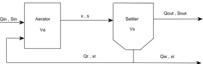
tor and achieves in the settler. In the settler thank, the solid components will settle and concentrate at the bottom whereas the sedimentation of soluble organic matter is assumed to be not significant. A part of bacteria biomass is recycled into aerator in order to stimulate the oxidation. The main three biological phenomena considered are : the reaction kinetics in the aerator linked to microbial growth, the substrate degradation and the recycle of the biomass from the settler. A schematic of the process is shown in Fig1.
Qin , Sin x , s Qr , xr Settler Vs Aerator Va Qw , xr Qout , Sout
Figure 1: Schematic diagram of the activated sludge process.
Where s, x and xrare the states variables representing respectively the substrate biomass
(pol-lutant), the bacteria biomass and recycled bacteria biomass concentrations. Qin, Qout, Qr, Qw are
the influent, effluent, recycle and waste flow rates, respectively. Va and Vs represent the aerator
and settler volumes and sincorresponds to the substrate concentrations in the feed stream. Due to
metabolic variations and the influence of many physical-chemical factors (PH, Temperature, oxy-gen, ...), it’s very hard to have an accurate idea of the specific growth function of the bacterium µ, (see [10, 11]). On the other hand, the substrate concentration in the feed stream sin fluctuates and
its variation depends on time and activities of the zone feeding the depuration station. Obviously, this situation incloses a very sensitive ecological problem, since due to fluctuations of µ and those of sin, the pollutant concentration may increase beyond the maximum tolerated level. Our goal in
this work is, firstly, to carry out a robust analysis of the model showing that, even if we consider that sin is constant and assume only that µ is not well known, (with given upper bound), the
sys-tem admit a domain of stability instead an unique global stable equilibrium point obtained in [16] when µ is perfectly known. Secondly, when both µ and sinare not known, we propose a design of
robust feedback control in term of recycle rate, in order to keep the system lower than a maximum allowed level sd. But, since µ and sinare not well known, concentrations of biomasses x, s and xr
are unmeasured and hence we can’t use theme to build the feedback control. Our approach consist to provide an upper observer of the system and through theory of monotone dynamical systems, we prove global partial stabilization of the upper observer of substrate concentration s about sd
and by the way keeping s ≤ sd. Many works are interested by similar problems where issues of :
optimal control [12, 13], observers [1, 2, 5, 9, 10, 12, 15], simulation [6, 14], have been studied. Robust control has been also treated, [4, 5, 7, 8], but without recycle biomass. Our approach is different : firstly, our system contain a recycle phenomena. Furthermore, we use the recycle rate as control instead of dilution rate D, often used as control, since this last variable is practical very hard to manipulate, and varying D implies variation of some other parameters as we will show
below. On the other hand, our control do not require the knowledge of online measurement of substrate concentration s.
2. Mathematical model
The basic model is developed in [3, 5, 10, 12]. The mass balance of the various constituents gives the following set of equations describing the evolution of substrate s, bacteria boimass x and recycle bacteria biomass xr :
(S) ˙s = −µ(s)x Y − (1 + r)Ds + Dsin; s(0) = s0 ˙x = µ(s)x − (1 + r)Dx + rDxr; x(0) = x0 ˙xr = ν(1 + r)Dx − ν(w + r)Dxr; xr(0) = xr0 with D := Qin Va
representing the dilution rate,
r := Qr Qin
representing the recycle rate,
w := Qw Qin
; ν := Va
Vs
,
and where Y refer to the yield coefficient of the growth of biomass on substrate. µ(.) is the specific growth function of the bacterium.
When all parameters are fully known and when sin is constant and µ is monotone increasing
(Monod type), we proved in Serhani et al. [16] that there exist an unique globally asymptotically stable equilibrium point. But generally, information about µ is not perfectly available, so, our goal in the next section is to investigate the situation where an upper bound of µ is handled.
Remark 1. As signaled in the introduction, the common tool through which a similar systems
(bioreactors and chemostat systems) are controlled in literature is the dilution rate D, see [4, 5, 7, 15]. But in our case, manipulating D implies the variation of Qin since Va is constant. This
fact leads to varying r and w since they depend also on Qin. This justify our choice, in this work
(section 5), of recycle rate r as control.
3. Robustness
The object of this section is to establish the existence of a global attractor interior domain when-ever full information about growth function µ is not available. We will carry out our study in the framework of the following assumptions :
3.1. Assumptions
We assume that :
A1 : D, sin, r, w, ν and Y are positive constants.
A2 : There exist µ : R+→ R+, monotone increasing and satisfying
•
0 ≤ µ(.) ≤ m ,
where m is a given constant representing the above bound of µ.
•
µ(s) = 0 if s = 0
•
µ(s) ≤ µ(s), ∀ s ≥ 0.
The classic example of µ, is the so-called Monod growth function, given by the following formu-lation :
µ(s) := ms b + s ,
where b is a constant representing the value at which µ takes the half of m.
Theorem 2. Assume that there exist s such that µ(s) = (1 + r)D w
w + r and that s < sin
1 + r, then
there exist x > 0 and xr > 0 such that, each trajectory of system (S) starting in R∗+3 converges
toward the domain D := {(s, x, xr) ∈ R+3 / (0, 0, 0) ≤ (s, x, xr) ≤ (s + Y x, x, xr)}.
Inequalities must be interpreted coordinate by coordinate.
Proof. Consider the variable change z := x + Y s, the system (S) can be reformulated to the system (Sc) given by (Sc) ˙z = −(1 + r)Dz + DY sin+ rDxr ; z(0) = z0 ˙x = µ(z−x Y )x − (1 + r)Dx + rDxr ; x(0) = x0 ˙xr = ν(1 + r)Dx − ν(w + r)Dxr ; xr(0) = xr0 ,
and consider the following systems :
(S) ˙z = −(1 + r)Dz + DY sin+ rDxr ; z(0) = z0 ˙x = µ(z−x Y )x − (1 + r)Dx + rDxr ; x(0) = x0 ˙xr = ν(1 + r)Dx − ν(w + r)Dxr ; xr(0) = xr0 , (S) ˙z = −(1 + r)Dz ; z(0) = z0 ˙x = −(1 + r)Dx ; x(0) = x0 ˙xr = −ν(w + r)Dxr ; xr(0) = xr0 .
It’s clear that (S) ≤ (Sc) ≤ (S) in the sense that the vector field of (Sc) is bounded above by the
vector field of (S) and below by one of the system (S). On the other hand, the jacobian matrices of the systems (S) and (S) are respectively given by
J(S) = −(1 + r)D 0 rD µ0(z − x Y ) x Y µ( z − x Y ) − µ 0(z − x Y ) x Y − (1 + r)D rD 0 ν(1 + r)D −ν(w + r)D , and J(S) = −(1 + r)D 0 0 0 −(1 + r)D 0 0 0 −ν(w + r)D .
Since the out-diagonal elements of these Jacobian matrices are nonnegative then systems (S) and (S) are cooperative (see [17] and [18]). Therefore, by using arguments of cooperatives inequalities (see [17] and [18]), we obtain that, if
u(t, u0) := {(z(t), x(t), xr(t)) ∈ R+3 / (z(0), x(0), xr(0)) = u0 := (z0, x0, xr0)},
is the flow of (Sc) and similarly u(t, u0) and u(t, u0) are respectively the flow of (S) and (S)
starting at the same point u0, then
u(t, u0) ≤ u(t, u0) ≤ u(t, u0), ∀ t ≥ 0. (3.1) On the other hand, in the system (S), the function µ is monotone increasing and
µ(s) = (1 + r)D w w + r ,
then by using analysis developed in [16] we know that there exist a non trivial, (i.e. not lying in boundaries), equilibrium point P = (z, x, xr) which is globally asymptotically stable for S, (this
means that all trajectories of system (S) starting in R∗
+3converges towards P ).
Moreover, it’s very easy to see that the system (S) has P = (0, 0, 0) as a globally asymptotically stable equilibrium point. To show this, it suffices to use the Lyapunov function
V := z2+ x2+ (xr)2.
So, according to (3.1) we conclude that all trajectories of system (Sc) starting from a point in R∗+3 converge toward the set
It remain to conclude for the system (S). Let (z, x, xr) be a trajectory of system (Sc). A trajectory
of (S) can be derived from these of (Sc) as
(s := z − Y x, x, xr).
Recall that
z ≤ z and x ≥ 0,
so, the substrate concentration s in the system (S) is such that,
s ≤ z ,
in other word,
s ≤ s + Y x, (3.2)
where s = z − Y x. Furthermore, we have that
x ≤ x and xr ≤ xr. (3.3)
On the other hand, the trajectory (s, x, xr) of system (S) is always nonnegative. Indeed, on the
axis
{(s, x, xr) ∈ R+3 / s = 0},
we have
˙s = Dsin,
so, ˙s is positive and hence the the vector field is pointed inside R+3. Similarly, on the axis
{(s, x, xr) ∈ R+3 / x = 0}, we have
˙x = rDxr ≥ 0,
which implies that the vector field ˙x is pointed inside R+3. Finally, on the axis
{(s, x, xr) ∈ R+3 / xr = 0},
we obtain
˙xr = ν(1 + r)Dx ≥ 0,
which also implies that the vector field ˙xris pointed inside R+3. It follows that, on the boundaries of R+3, the vector field ( ˙s, ˙x, ˙xr) is pointed inside the positive octant and hence each trajectory
(s, x, xr) of system (S) is such that
(s(t), x(t), xr(t)) ≥ 0, ∀ t ≥ 0. (3.4)
We conclude from (3.2), (3.3) and (3.4), that all trajectories of the system (S) converge toward the domain
as required.
From the last analysis it follows that even if we suppose that the recycle rate r and the substrate concentration in the feed stream sin are known constants and an upper bound of µ is given, the
system admit a domain of stability, instead an unique global stable equilibrium point arising when
µ is perfectly known, ([16]). This situation incloses some difficulties, since, firstly, sin and the
boundary of µ are in general not well known. Secondly the fluctuations of the growth function
µ and pollutant concentration level s and hence the s−boundary of domain D may exceed the
maximum level tolerated by environment. Our goal in next sections is to control the recycle rate r in order to keep s lower than an allowed maximum level.
4. Upper observer of pollutant concentration
4.1. Hypotheses
Let us now formulate the new assumptions under which we will work along the rest of this work.
H1− The coefficients D, w, Y and ν are assumed to be positive constants.
H2− The recycled rate r(t) is a known nonnegative bounded time varying function.
H3− We assume that µ is not known.
H4− sin(t) is a not well known time varying function but bounded above by :
sin(t) ≤ s+in, ∀t ≥ 0 ,
where s+
inis a given positive constant.
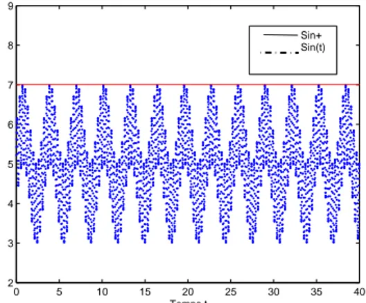
During the simulations in the section (6.), to be in the framework of the hypothesis H3, we have choose a function µ with an expression, (equation (6.1)), involving oscillations, nonsmoothness and inhibition. This fact is illustrated by the figure (2). Similarly, the hypothesis H4 is taken into account in simulation, thanks to sin(t) and s+in, given respectively by equations (6.2) and (6.3).
sin(t) oscillate between a known bounds for which the upper bound is s+inas shown in figure (3).
4.2. Observer
To build a feedback control in term of recycle rate r(t), it requiring to have a perfect knowledge of variables involved for this construction. But in practice, it is very hard to have a full information of bioprocess kinetics, so, an accurate data is not available, due to metabolic variations and the influ-ence of many physic-chemical factors. The purpose of this section is to derive an upper observer which permit us to have an estimation of the upper bound of missing data.
Consider the following system
(Sup) ˙s+ = −D(1 + r(t))s++ Ds+ in; s+(0) = s+0 ˙x+= µ(s+)x+− (1 + r)Dx++ rDx+ r ; x+(0) = x+0 ˙x+ r = ν(1 + r)Dx+− ν(w + r)Dx+r ; x+r(0) = x+r0 ,
we obtain an upper observer of the system (S).
Theorem 3. For given nonnegative vectors (s+
0, x+0, x+r0) and (s0, x0, xr0) such that (s0, x0, xr0) ≤
(s+
0, x+0, x+r0), we have
s(t) ≤ s+(t) , x(t) ≤ x+(t) , x
r(t) ≤ x+r(t) , ∀t ≥ 0 . (4.1)
Where (s(t), x(t), xr(t)) and (s+(t), x+(t), x+r(t)) are the vector fields of systems (S) and (Sup)
respectively with initial conditions (s0, x0, xr0) and (s+0, x+0, x+r0) respectively.
Proof. Let p(t) = (p1(t), p2(t), p3(t)) ∈ R+3 , ∀ t ≥ 0 and q(t) = (q1(t), q2(t), q3(t)) ∈
R3+, ∀ t ≥ 0. By choosing f (t, p(t)) := −µ(p1(t)) Y p2(t) − (1 + r)Dp1(t) + Dsin µ(p1(t))p2(t) − (1 + r)Dp2(t) + rDp3(t) ν(1 + r)Dp2(t) − ν(w + r)Dp3(t) and g(t, q(t)) := −D(1 + r)q1(t) + Ds+in µ(q1(t))q2(t) − (1 + r)Dq2(t) + rDq3(t) ν(1 + r)Dq2(t) − ν(w + r)Dq3(t) . The systems (S) and (Sup) can be rewritten as
˙p(t) = f (t, p(t)) ; p(0) = p0 (4.2) and ˙q(t) = g(t, q(t)) ; q(0) = q0 (4.3) Where p(t) = (s(t), x(t), xr(t)) , q(t) = (s+(t), x+(t), x+r(t)) , ∀ t ≥ 0 , and p0 = (s0, x0, xr0) , q0 = (s+0, x+0, x+r0).
It’s clear, according to hypothesis H4, that for all t, p(t) ≥ 0 ,
f (t, p(t)) ≤ g(t, p(t)).
Hence, we obtain, according to cooperative property of system 4.3, that, for a vectors fields p and
q of systems 4.2 and 4.3 respectively, if the initial conditions satisfying p0 ≤ q0then the following inequality holds
We conclude according to this last inequality (4.4) and the fact (s0, x0, xr0) ≤ (s+0, x+0, x+r0), that s(t) ≤ s+(t) , x(t) ≤ x+(t) , x r(t) ≤ x+r(t) , ∀t ≥ 0 , as required.
5. Control action
The main of this section is to resolve the following question (Q) :
Given a initial condition (s0, x0, xr0) ∈ R3∗+, find a feedback control, in term of recycle rate r(t),
to ensure that, for any unknown µ and sin fulfilling H3 and H4, the pollutant concentration s of
system (S) be lower than a maximum fixed level sd.
Let the feedback law r given by the following expression
r(s+, s+in) = 1 sd (s+in− sd) , if s+< sd 1 Ds+[(s + in− s+)D + λ(s+− sd)] , if s+ ≥ sd, (5.1)
where s+is the upper observer of s given by (4.2.) and λ ∈ R.
To simplify notation we will use the notation r(t). Let us first prove that r(t) is nonnegative and bounded.
Proposition 4. If sd < s+in(t) and λ > D then the control r(t) given by (5.1), is nonnegative and
bounded.
Proof. If s+ ≤ s
dthen r(t) =
1
sd
(s+in− sd), but since sd≤ s+in, we obtain that r(t) ≥ 0 .
Now if s+> s dthen r(t) = 1 Ds+[(s + in− s+)D + λ(s+− sd)] . We have that r(t) ≥ 0 if (s+in− s+)D + λ(s+− sd) ≥ 0 , which is equivalent to λ ≥ Ds+(t) − s + in(t) s+(t) − s d , ∀t ≥ 0 . It suffices to choose λ ≥ maxt≥0{D s+(t) − s+ in(t) s+(t) − s d } = D .
Therefore, to have r(t) ≥ 0, it suffice to choose
λ ≥ D ,
which is the case by assumption.
The fact that r(t) is bounded, is obtained by studying variation of r(t) with respect s+. By simple arguments of real functions variation study, we obtain that, if λ ≥ s
+ in sd , then r(t) ∈ [λ − D, s + in− sd sd ] , and if λ ≤ s + in sd , then r(t) ∈ [s + in− sd sd , λ − D] , as required.
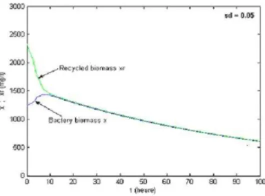
The nonnegativity of the feedback control indicates that our choice is correct while the fact that it is bounded is very important since, in practice the quantities recycled are finished. Those properties are illustrated through simulations, in the next section, for two choices of the parameter sd (sd =
0.5 and sd= 0.05), see figure (8).
Now we give our mean result.
Theorem 5. With feedback control r(t) given by equation (5.1), there exist T ≥ 0, such that, for
all t ≥ T , s(t) ≤ sd.
Where s is the biomass concentration of substrate.
Proof. The idea is to stabilize the upper observer s+about s
d, and since s(t) ≤ s+(t), ∀t ≥ 0, we
obtain that s(t) ≤ sd, ∀t ≥ 0. Prove now that with the choice of the recycle rate r(t) as given by
equation (5.1), s+is globally asymptotically stable about s
d.
Consider the Lyapunov function
V (s+) := (s+− s
d)2.
V is nonnegative and V (sd) = 0.
Prove now that dV
dt (s +) < 0, for all s+ 6= s d. dV dt (s +) = 2(s+− s d) d dts + = 2(s+− s d)(−D(1 + r(t))s++ Ds+in(t)) . If s+< s dthen r(t) = 1 sd (s+ in− sd).
It follows that, dV dt = 2(s +− s d)(−D s+ in sd s++ Ds+ in) = 2(s+− s d)Ds+in(− s+ sd + 1) . But, s+ sd < 1, then, since (s+− s d) < 0 and − s+ sd + 1 > 0, we obtain that dV dt (s +) < 0, ∀s+ 6= s d, as required. If now s+≥ s dthen r(t) = 1 Ds+[(s + in− s+)D + λ(s+− sd)] . So, dV dt (s +) = −2λ(s+− s d)2 < 0 , ∀s+ 6= sd, as required.
The simulations in the next section (6.) give an illustration of the theoretical investigations of the previous theorem. Firstly, the fact that the upper observer s+ can be stabilized about s
d, through
the feedback control (5.1), (as established in the proof of the previous theorem), is illustrated by the figure (4) in which we show that s+is stabilizated about s
dfor two values : sd= 0.5 and sd = 0.05.
On the other hand, the figure (5) illustrate the result of the previous theorem and shows that the substrat s is keeping below the allowed level sd, (for sd = 0.5 and sd = 0.05). Finally, figures (6)
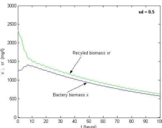
and (7) show the evolution of the bacteria biomass x and recycle biomass xr in time when we use
the feedback control r given by equation (5.1), for respectively sd = 0.05 and sd= 0.5.
6. Numerical simulations
Simulation results are obtained for the following specific growth function
µ(s) := 400s 75 + s + s 2 100 | sin(s)| + s 20sin(2s) , (6.1)
In this choice, the sinus function is used to produce periodicity and absolute value is used to produce non smoothness and finally the quadratic term to produce inhibition.
The concentration in feed stream is given by
An upper bound, s+
in, of sin(t) can hence be equal to
s+in= 7 (6.3)
The model parameters and initial conditions are given as follows :
D = 0.3; Y = 0.8; ν = 2; w = 0.5; x0 = 1225; xr0 = 2333; s0 = 20; λ = 2; s+0 = 30.
Figure 2: Variation of the unknown specific growth function µ(.).
0 5 10 15 20 25 30 35 40 2 3 4 5 6 7 8 9 Temps t Sin+ Sin(t)
Figure 4: Graph of upper observer s+.
Figure 5:Graph of pollutant concentration s.
Figure 7: Bacterium biomass and recycled biomass for (sd = 0.5).
7. Conclusion
This work is interested by an activated sludge problem. We developed a robust analysis when the specific growth function of the bacteria µ is not well known, leading to existence of a stability domain. When also the substrate concentrations in the feed stream sin is not known, we built a
feedback control, in terms of recycle rate r(.), depending on an observer of bacteria concentration
s (pollutant), in order to keep this last variable below than an allowed maximum level sd.
8. Acknowledgements
We are grateful to the anonymous referee for his valuable comments suggestions and remarks.
References
[1] V. Alcaraz-Gonzalez, J. Harmand, A. Rapaport, J.-P. Steyer, V. Gonzalez Alvarez, C. Pelayo Ortiz. Application of a robust interval observer to an anaerobic digestion process. Develop-ments in Chemical Engineering Mineral Processing, 13 (2005), No. 3/4, 267–278.
[2] V. Alcaraz-Gonzalez, J. Harmand, A. Rapaport, J.-P. Steyer, V. Gonzalez Alvarez, C. Pelayo Ortiz. Robust interval-based regulation for anaerobic digestion processes. Water Science and Technology, 52 (2005), No. 1-2, 449–456.
[3] J.F. Andrews. Kinetic models of biological waste treatment process. Biotech. Bioeng. Symp., 2 (1971), 5–34.
[4] J.F. Andrews. Dynamics and control of wastewater systems. Water quality management li-brary, vol. 6, 1998.
[5] J.F. Busb, J.F. Andrews. Dynamic modelling and control strategies for the activated sludge
process. J. of Wat. Pollut. Control Fed., 47 (1975), 1055–1080.
[6] C.R. Curds. Computer simulation of microbial population dynamics in the activated sludge
process. Water Research 5 (1971), 1049–1066.
[7] D. Dochain, M. Perrier. Control design for nonlinear wastewater treatment processes. Wat. Sci. Tech. 11-12 (1993), 283–293.
[8] D. Dochain, M. Perrier. Dynamical modelling, analysis, monitoring and control design for
nonlinear bioprocess. T. Scheper (Ed.), Advances in Biochemical and Biotechnology, 56
[9] C. G´omez-Quintero, I. Queinnec. Robust estimation for an uncertain linear model of an
acti-vated sludge process. Proc. of the IEEE Conference on Control Applications (CCA), Glasgow
(UK), (2002), 18-20 december.
[10] M.Z. Hadj-Sadok, J.L. Gouz´e. Estimation of uncertain models of activated sludge processes
with interval observers. J. of Process Control, 11 (2001), 299–310.
[11] B. Haegeman, C. Lobry, J. Harmand. Modeling bacteria flocculation as density-dependent
growth. Aiche Journal, 53 (2007), No.2, 535–539.
[12] S. Marsili-Libelli. Optimal control of the activated sludge process. Trans. Inst. Meas. Control, 6 (1984), 146–152.
[13] A. Mart´ınez, C. Rodr´ıguez, M.E. V´azquez-M´endez. Theoretical and numerical analysis of
an optimal control problem related to wastewater treatment. SIAM J. CONTROL OPTIM.,
Vol. 38 (2000), No. 5, 1534–1553.
[14] M.K. Rangla, K.J. Burnham, L.Coyle, R.I.Stephens. Simulation of activated sludge process
control strategies. Simulation ’98. International Conference on (Conf. Publ. No. 457), 30 Sep
- 2 Oct (1998), 152–157.
[15] A. Rapaport, J. Harmand. Robust regulation of a class of partially observed nonlinear
con-tinuous bioreactors. J. of Process Control, 12 (2002), No. 2, 291–302.
[16] M. Serhani, J.L. Gouz´e, N. Ra¨ıssi. Dynamical study and robustness for a nonlinear
wastew-ater treatment model. Proceeding book ”Systems Theory : Modeling, Analysis & Control,
FES2009”, Eds A. EL Ja¨ı, L. Afifi & E. Zerrik, PUP, ISBN 978-2-35412-043-6, pp. 571-578.
[17] H.L. Smith. Monotone dynamical systems : an introduction to the theory of competitive and
cooperative systems. American Matheatical society, 1995.
[18] H.L. Smith, P. Waltman. The theory of the chemostat. Cambridge University Press, Cam-bridge, 1995.