HAL Id: hal-03016527
https://hal.archives-ouvertes.fr/hal-03016527
Submitted on 20 Nov 2020HAL is a multi-disciplinary open access
archive for the deposit and dissemination of sci-entific research documents, whether they are pub-lished or not. The documents may come from teaching and research institutions in France or abroad, or from public or private research centers.
L’archive ouverte pluridisciplinaire HAL, est destinée au dépôt et à la diffusion de documents scientifiques de niveau recherche, publiés ou non, émanant des établissements d’enseignement et de recherche français ou étrangers, des laboratoires publics ou privés.
Enhanced future warming constrained by past trends in
the equatorial Pacific sea surface temperature gradient
Masahiro Watanabe, Jean-Louis Dufresne, Yu Kosaka, Thorsten Mauritsen,
Hiroaki Tatebe
To cite this version:
Masahiro Watanabe, Jean-Louis Dufresne, Yu Kosaka, Thorsten Mauritsen, Hiroaki Tatebe. En-hanced future warming constrained by past trends in the equatorial Pacific sea surface temperature gradient. Nature Climate Change, Nature Publishing Group, 2020, �10.1038/s41558-020-00933-3�. �hal-03016527�
1
Enhanced future warming constrained by past trends in the
equatorial Pacific sea surface temperature gradient
Masahiro Watanabe1*, Jean-Louis Dufresne2, Yu Kosaka3, Thorsten Mauritsen4 & Hiroaki
Tatebe5
1: Atmosphere and Ocean Research Institute, University of Tokyo, Chiba, Japan
2: Laboratoire de Météorologie Dynamique, Institut Pierre et Simon Laplace, Paris, France 3: The Research Center for Advanced Science and Technology, the University of Tokyo, Tokyo,
Japan
4: Department of Meteorology, Stockholm University, Stockholm, Sweden 5: Japan Agency for Marine-Earth Science and Technology, Kanagawa, Japan
* Corresponding author:
Masahiro Watanabe, Atmosphere and Ocean Research Institute, the University of Tokyo, 5-1-5 Kashiwanoha, Kashiwa, Chiba 277-8568, Japan.
Phone: 81-4-7136-4387, Fax: 81-4-7136-4375 E-mail: [email protected]
Nature Climate Change
The zonal gradient in the equatorial Pacific sea surface temperature (SST), high in the
1
west and low in the east, is known to be a pacemaker of global warming1. The zonal SST 2
gradient has strengthened since the mid-20th century2, but the cause is controversial 3
because it is not reproduced by a majority of Coupled Model Intercomparison Project
4
Phase 5 (CMIP5) climate models3–6, which instead suggest a weakening of the zonal SST 5
gradient from the past to the future7. This discrepancy between observations and models 6
has to be reconciled not only for attributing the past climate change but also for assessing
7
Earth’s climate sensitivity8,9. Here we show using large ensemble (LE) simulations by four 8
different climate models, in addition to CMIP5 models, that the intensified trend in the
9
Pacific zonal SST gradient for 1951–2010 can be captured by some realisations,
10
suggesting that it could arise from internal climate variability. Models and members that
11
simulate the past strengthening of the SST gradient in CMIP5 and LE commonly exhibit
12
reversed trends in future projections, when the rate of global-mean temperature rise is
13
likely to amplify by 9–30% with the larger values occurring in low-emission scenarios.
14
Atmosphere-ocean state in the tropical Pacific is characterised by the zonal contrast
15
between high SST in the warm pool and low SST in the cold tongue, tied with the Walker
16
circulation accompanying surface easterlies. This mean state is maintained by the well-known
17
Bjerknes feedback10, which acts against radiative heating that homogenises SST zonally.
18
Specifically, equatorial easterlies pile warm water up to the west and cause upwelling to cool
19
the eastern Pacific. The strengthened SST gradient, in turn, amplifies the easterlies by
3
enhancing atmospheric convection over the warm pool that excites the zonal gradient in sea
21
level pressure. The same feedback explains how El Niño–Southern Oscillation (ENSO) can be
22
excited at interannual time scales11,12. Because of the ENSO variability, detecting longer term
23
changes in the zonal SST gradient in 20th century observations remains a challenge.
24
In future projections by CMIP5 Representative Concentration Pathways (RCP)
25
simulations13, SST in the equatorial central–eastern Pacific warms more than the western
26
Pacific with a certain degree of uncertainty7,14,15, and the change is sometimes referred to as
27
the ‘El Niño-like’ pattern. There are several hypotheses that explain the long-term SST pattern
28
change; an ocean dynamical thermostat which prevents excessive warming in the warm pool16
29
and surface wind-evaporation-SST feedback suppressing the western basin warming17. The
30
weakening of the zonal SST gradient in future projections is coupled with a slowdown of the
31
Walker circulation, which has been supported from both a theory18 and climate model
32
simulations19,20.
33
The CMIP5 historical simulations similarly show the weakening of the SST gradient
34
during the 20th century3. However, it is not supported by observations, which commonly show
35
that the SST gradient has strengthened since the middle of the 20th century2 (Supplementary
36
Fig. 1), consistent with a strengthening of the Walker circulation as suggested from atmospheric
37
data21. There exist observational uncertainty22 and a dependence of the trend magnitude on
38
chosen period6, but the discrepancy between observations and climate models is obvious and
39
critical not only for assessing the reliability of future climate changes in models but also for
4
estimating the Earth’s climate sensitivity (ECS) from historical records. Recent studies show
41
that cloud and lapse rate feedbacks to doubling of CO2 concentration depend on spatial
42
inhomogeneity in sea surface warming8,9,23, called the ‘pattern effect’ 24. Specifically, if the
43
SST gradient in the tropical Pacific is strengthened, these feedbacks tend to be weak or change
44
the sign from positive to negative, leading to a low estimate of ECS, and vice versa. Thus,
45
reconciling past zonal SST gradient change may aid in narrowing the range of ECS estimates
46
from historical observations and CMIP5 models.
47
The observed strengthening of the Pacific zonal SST gradient can be due to either an
48
internal variability of the climate system or a forced response to greenhouse gases (GHGs) and
49
other agents such as aerosols and solar activity. On one hand, individual model simulations do
50
not necessarily reproduce observations if internal variability is the main driver of the observed
51
trend, which should instead be covered by the whole ensemble. On the other hand, the model
52
ensemble mean will capture the observed trend if it is attributable to the external radiative
53
forcing given a possibility that cooling by the mean upwelling in the cold tongue retards the
54
transient warming in this region. Both these cases however may not apply when models have
55
biases due to systematic errors. A similar discussion has continued for understanding the cause
56
of the global warming ‘hiatus’ 25 that lasted about 15 years since around 2000. The differences
57
lie in the length of the linear trend (60 years for the present analysis), and the increasing
58
influence of radiative forcing is expected at this time scale.
5
Analyses of the CMIP5 historical simulations show that the observed strengthening of the
60
zonal SST gradient is outside of the ensemble of simulated trends, suggesting a primary role of
61
external forcing whose impact is not adequately calculated in climate models3,4. A recent study,
62
based on simulations using a simplified atmosphere-ocean model with observed mean states,
63
concluded that the GHG-forced response in CMIP5 models would be consistent with the
64
observations if the bias in mean SST, which is too cold in the eastern Pacific, did not exist5.
65
However, this conclusion raises another inconsistency with our current understanding that the
66
SST gradient (and the Walker circulation) would be weakened in the long-term response to
67
global warming14. Furthermore, it is plausible that the ensemble of opportunity by CMIP5
68
simulations insufficiently samples the spread due to internal variability. Indeed, increased
69
number of realisations, using either long pre-industrial control runs or a large set of historical
70
simulations by a single climate model, made it possible to include ensemble members that show
71
both weakening and strengthening of the Walker circulation, the latter being similar to the
72
observed feature6,26.
73
To examine whether the observed changes in the equatorial Pacific zonal SST gradient,
74
hereafter denoted as SSTeq (east minus west, see Methods), reflect internal variability, we
75
analysed a combined set of large ensembles (LEs) from four different climate models having
76
220 members in total, in addition to CMIP5 historical runs, and compared them with six SST
77
data sets (Methods). Each LE consists of historical runs made by perturbing the initial condition
78
and thus the ensemble deviations solely represent internal variability. We demonstrate that the
6
large set of simulations covers well the observed trend of SSTeq for 1951–2010 although the 80
ensemble shows a bias towards weakening SSTeq; the result indicates that the observed 81
strengthening of the SST gradient can be caused by internal variability at the interdecadal time
82
scale. Furthermore, the SST gradient will turn to a weakening by the end of this century in all
83
RCP scenarios, during which a rate of global-mean surface air temperature (GSAT) increase is
84
temporarily amplified.
85
In the four equatorial ocean strips (Indian Ocean, western and eastern Pacific, and Atlantic),
86
observed SST has increased by about 0.6 K over 1951–2010 (Supplementary Fig. 2). It is well
87
reproduced by the CMIP5 ensemble-mean anomalies except for the eastern Pacific where
88
models overestimate the observed warming: 1.1 versus 0.78 K per century. While the
89
differences in observed and simulated SST trends are apparently small, the trend in SSTeq is 90
quite distinct; all observational data sets show the negative trend but only a few models do the
91
same (Fig. 1a and Supplementary Fig. 3). The observed SSTeq trend is robust when shifting 92
the 60-year period from 1951–2010 to 1960–2019 (Supplementary Fig. 4), but the magnitude
93
is systematically different between interpolated analyses (HadISST, COBE-SST2, ERSSTv5,
94
Kaplan) and un-interpolated data sets (HadSST3 and ICOADS). The ensemble of six data sets
95
leads to the value of –0.33±0.16 K per century (the range representing the standard deviation),
96
which may overestimate the true trend given potential errors in the SST analysis22.
97
While CMIP5 models show a large inter-model spread, the average of the observed
98
SSTeq trends is outside the 5–95% range of the CMIP5-based trends (bars in Fig. 1b). This is
7
apparently consistent with the argument that models fail to represent the externally forced
100
signal, which may explain the observed SSTeq trend4,5. However, probability distributions of 101
SSTeq trends from 220-member LEs, calculated for individual models, capture the
102
observations (Fig. 1b). The ensemble-mean trends are either positive or negative among the
103
four LEs, indicating a model uncertainty in the externally forced response. Whereas the
104
agreement with the IPSL-CM6A-LR and MIROC6 ensembles are only marginally consistent
105
with observations, CESM1 and MPI-ESM1.1 show 10 and 40% of the ensemble members
106
exceeding the observed SSTeq trend. Thus, the CMIP5 ensemble clearly underestimates the
107
uncertainty range arising from natural internal variability, and LEs suggest that the observed
108
negative SSTeq trend can be caused by internal variability at the interdecadal time scale. The 109
features found in Fig. 1 change little when interannual ENSO signals were removed before
110
calculating the linear trends (Methods and Supplementary Fig. 5).
111
As Bjerknes feedback operates at any time scale, the change in ocean subsurface
112
temperature should be different between models that reproduce or fail the observed SSTeq 113
trend. When we select six CMIP5 models that show the SST gradient strengthening (called
S-114
models) and also weakening (W-models), we see a contrast in their means and spreads: –
115
0.24±0.1 and 0.39±0.1 K per century (red and blue bars in Fig. 1a). Linear trends in the
116
equatorial ocean temperature for 1951–2010 from observations, CMIP5 ensemble mean, and
117
averages of S- and W-models, reveal an intriguing difference in addition to an overall similarity
118
(Fig. 2).
8
The most prominent feature of the observed ocean temperature trend is the contrast
120
between warming near the surface and cooling near the thermocline (Fig. 2a). The subsurface
121
cooling is indicative of a rising of the thermocline from the dateline to the eastern Pacific. This
122
causes the upwelling to cool the surface layer in the eastern basin, consistent with the negative
123
SSTeq trend. The CMIP5 ensemble-mean trend qualitatively simulates this subsurface
124
cooling, which is regarded as a forced oceanic response (Fig. 2b). The shoaling trend of the
125
equatorial thermocline has been reported in the literature7 and is accompanied by a deepening
126
of the thermocline in subtropical oceans as measured by the trend in a depth of 20 °C isotherm
127
in both observations and the CMIP5 ensemble mean (Supplementary Fig. 6).
128
Compared to the vertical structure of the observed temperature trend, the surface layer is
129
thicker besides subsurface cooling weaker and shifted to a deeper layer in the CMIP5 ensemble
130
mean. These models suggest that the upwelling does not effectively cool the eastern Pacific
131
despite the rising of the thermocline. This is more clearly identified in W-models where
132
subsurface cooling occurs only weakly in the western Pacific, in contrast to a large subsurface
133
cooling in the eastern Pacific seen in S-models (Fig. 2c, d). The difference between S- and
W-134
models may partly be attributed to a different structure of the externally forced response, but a
135
quite similar contrast in the magnitude and location of subsurface cooling has been identified
136
by categorising CESM1 LE into members that show a strengthening and a weakening of the
137
Walker circulation25. This suggests that the difference between S- and W-models is primarily
138
due to the effect of internal variability.
9
A dominant low-frequency mode of internal variability in the Pacific is the Interdecadal
140
Pacific Oscillation (IPO), featuring a similar spatial pattern to ENSO but modulating the
141
eastern Pacific SST and hence SSTeq at interdecadal time scales27 (Supplementary Figs. 7-9).
142
The phase of the IPO varies irregularly28 and has changed more than once during 1951–2010
143
in both observations and each member of the historical ensemble. However, S-models tend to
144
show a positive phase in the early period and a negative phase in the late period, and vice versa
145
for W-models. The difference in the IPO trend is subtle, but it is clearer in the MPI LE. While
146
irregularity of the IPO results in uncertainty to a certain degree, its turnabout is expected to
147
occur in coming decades. The IPO phase reversal, in addition to the forced ‘El Niño-like’
148
pattern in future projections, is likely to amplify the positive SSTeq trend for 2001–2050 in 149
S-models but suppress it in W-models (Supplementary Fig. 10).
150
Indeed, the linear SSTeq trends calculated using 50-year moving segments change the 151
sign from negative to positive by the mid-21st century in S-models while they are positive
152
throughout the period in W-models; their difference is maximum for 1991–2040 (Fig. 3a).
153
Because the IPO predictability is less than a decade29, this result does not indicate that the
154
future phase of the IPO can be predicted by its past state but rather suggests that the recovery
155
from negative or positive phase during the historical period influences the future multi-decadal
156
trend in SSTeq. A very similar result was obtained from a single LE using MPI-ESM1.1, 157
supporting the premise that near-term change in SSTeq is modulated by internal variability 158
(Fig. 3b). In both CMIP5 and the MPI LE, the SSTeq trends are not well separated between
10
S- and W-groups in the late 21st century. This indicates that the amplification of weakening the
160
SST gradient is a temporary phenomenon.
161
Previous debates on the global warming hiatus have made it clear that the equatorial
162
Pacific SST pattern, as measured by SSTeq, is an important driver of GSAT to slow down or
163
accelerate the radiatively forced response1,21,25,30. Therefore, the evolution of multi-decadal
164
trends in GSAT is expected to reveal a discernible difference between S- and W-models (Fig.
165
4). Consistent with the reversal of the SSTeq trend in the future, a positive GSAT trend in S-166
models is larger than in W-models in all the RCP simulations, although the timing of this
167
amplified global warming is dependent on the scenarios. In a stabilisation scenario of RCP2.6,
168
the rates of warming are clearly different between S- and W-models (larger in the former than
169
the latter) by about 2050, but the difference eventually diminishes thereafter (Fig. 4a). With a
170
strong GHG forcing in RCP8.5, the difference in GSAT trend between S- and W-models
171
appears throughout the century (Fig. 4c). Yet, the implications of attributing historical changes
172
in zonal SST gradient is evident; the rate of global warming will be temporarily amplified if
173
climate models reproduce the observed strengthening of the SST gradient for 1951–2010.
S-174
models show the greatest amplification in the 50-year trend by 29.6% in RCP2.6 for 1981–
175
2030 while the least by 8.9% in RCP8.5 for 2051–2100. This dependence on scenario can be
176
interpreted in terms of the signal-to-noise ratio; the influence of internal variability (noise) on
177
future warming rates is larger if the GHG-induced warming (signal) is smaller.
11
The small inter-model spread of the SSTeq trend in CMIP5 may be partly due to an 179
underestimation of the SST variance associated with the IPO28,31 (Supplementary Figs. 8 and
180
11). The four LEs except IPSL-CM6A-LR simulate the IPO with a larger amplitude than many
181
CMIP5 models, and it might be a reason why LEs successfully captured the observed SSTeq
182
trend.
183
Our results do not exclude the possibility that climate models systematically fail to
184
simulate a forced component in the SSTeq trend5 given that the observed large trend lies 185
outside the CMIP5 range (Fig. 1). This may not happen due solely to an extreme internal
186
fluctuation at interdecadal time scales6. However, additional analyses show that the failure to
187
reproduce the observed trend only spans over the recent two decades, but not the entire 60-year
188
period (Supplementary Figs. 12 and 13). For 1991–2010, the observed SSTeq trend is far 189
stronger than the simulated trends in CMIP5 and even any of LEs. This period corresponds to
190
the hiatus when the Pacific trade winds were stronger than ever since the early 20th century21.
191
The intensified SSTeq trend for 1991–2010, 15 times as large as the trend for 1951–2010, has 192
been suggested to be forced partially by sulphate aerosols32 or the Atlantic warming33. Although
193
such a process might have not been represented by climate models well, our results indicate
194
that considering internal climate variability is critical for understanding long-term changes in
195
the Pacific zonal SST gradient and global-mean temperature not only for the past decades but
196
also for the future projection.
197 198
12
References
199
1. Kosaka, Y. & Xie S.-P. The tropical Pacific as a key pacemaker of the variable rates of
200
global warming. Nature Geosci. 9, 669–673 (2016).
201
2. Solomon, A. & Newman, M. Reconciling disparate twentieth-century Indo-Pacific Ocean
202
temperature trends in the instrumental record. Nat. Clim. Change 2, 691–699 (2012).
203
3. Coats, S. & Karnauskas, K. B. Are simulated and observed twentieth century tropical
204
Pacific sea surface temperature trends significant relative to internal variability? Geophys.
205
Res. Lett. 44, 9928–9937 (2017).
206
4. Luo, J.-J., Wang, G. & Dommenget, D. May common model biases reduce CMIP5’s ability
207
to simulate the recent Pacific La Niña-like cooling? Clim. Dynam. 50, 1335–1351 (2018).
208
5. Seager, R., Cane, M., Henderson, N. et al. Strengthening tropical Pacific zonal sea surface
209
temperature gradient consistent with rising greenhouse gases. Nat. Clim. Change 9, 517–
210
522 (2019).
211
6. Bordbar, M. H., Martin, T., Latif, M. & Park, W. Role of internal variability in recent
212
decadal to multidecadal tropical Pacific climate changes. Geophys. Res. Lett. 44, 4246–
213
4255 (2017).
214
7. Collins, M., An, S., Cai, W. et al. The impact of global warming on the tropical Pacific
215
Ocean and El Niño. Nature Geosci. 3, 391–397 (2010).
13
8. Andrews, T., Gregory, J. M., Paynter, D. et al. Accounting for changing temperature
217
patterns increases historical estimates of climate sensitivity. Geophys. Res. Lett. 45, 8490–
218
8499 (2018).
219
9. Ceppi, P. & Gregory, J. M. Relationship of tropospheric stability to climate sensitivity and
220
Earth’s observed radiation budget. Proc. Nat. Acad. Sci. 114, 13126–13131 (2017).
221
10. Bjerknes, J. Atmospheric teleconnections from the equatorial Pacific. Mon. Weather Rev.
222
97, 162–172 (1969).
223
11. Jin, F.-F. Tropical ocean-atmosphere interaction, the Pacific cold tongue, and the El Niño
224
Southern Oscillation. Science 274,76-78 (1996).
225
12. Timmermann, A., An, S.-I., Kug, J.-S. et al. El Niño–Southern Oscillation complexity.
226
Nature 559, 535–545 (2018).
227
13. Taylor, K. E., Stouffer, R. J. & Meehl, G. A. An overview of CMIP5 and the experiment
228
design. Bull. Amer. Meteor. Soc. 93, 485–498 (2012).
229
14. Christensen, J. H. et al. Climate phenomena and their relevance for future regional Climate
230
change. In: Climate Change 2013: The Physical Science Basis. Contribution of Working
231
Group I to the Fifth Assessment Report of the Intergovernmental Panel on Climate Change.
232
Stocker, T. F. et al. (eds.), Cambridge University Press (2013).
233
15. Kim, S. T., Cai, W., Jin, F.-F. et al. Response of El Niño sea surface temperature variability
234
to greenhouse warming. Nat. Clim. Change 4, 786–790 (2014).
14
16. Clement, A., Seager, R., Cane, M. A. & Zebiak, S. E. An ocean dynamical thermostat. J.
236
Climate 9, 2190–2196 (2019).
237
17. Xie, S.-P., Deser, C. Vecchi, G. A. et al. Global warming pattern formation: Sea surface
238
temperature and rainfall. J. Climate 23, 966–986 (2010).
239
18. Held, I. M. & Soden, B. J. Robust responses of the hydrological cycle to global warming.
240
J. Climate 19, 5686–5699 (2006).
241
19. Vecchi, G. A., Soden, B. J., Wittenberg, A. T. et al. Weakening of tropical Pacific
242
atmospheric circulation due to anthropogenic forcing. Nature 441, 73–76 (2006).
243
20. Chadwick, R., Boutle, I. & Martin, G. Spatial patterns of precipitation change in CMIP5:
244
Why the rich do not get richer in the tropics. J. Climate 26, 3803–3822 (2013).
245
21. England, M. H., McGregor, S., Spence, P. et al. Recent intensification of wind-driven
246
circulation in the Pacific and the ongoing warming hiatus. Nat. Clim. Change 4, 222–227
247
(2014).
248
22. Deser, C., Phillips, A. S. & Alexander, M. A. Twentieth century tropical sea surface
249
temperature trends revisited. Geophys. Res. Lett. 37, L10701 (2010).
250
23. Zhou, C., Zelinka, M. D. & Klein, S. A. Impact of decadal cloud variations on the Earth’s
251
energy budget. Nat. Geosci. 9, 871–874 (2016).
252
24. Dong, Y., Proistosescu, C., Armour, K. C & Battisti, D. S. Attributing historical and future
253
evolution of radiative feedbacks to regional warming patterns using a Green’s function
254
approach: The preeminence of the western Pacific. J. Climate 32, 5471–5491 (2019).
15
25. Fyfe, J. C., Meehl, G. A., England, M. H. et al. Making sense of the early-2000s warming
256
slowdown. Nat. Clim. Change 6, 224–228 (2016).
257
26. Chung, E.-S., Timmermann, A., Soden, B. J. et al. Reconciling opposing Walker
258
circulation trends in observations and model projections. Nat. Clim. Change 9, 405–412
259
(2019).
260
27. Power, S., Casey, T., Folland, C. et al. Inter-decadal modulation of the impact of ENSO on
261
Australia. Clim. Dynam. 15, 319–324 (1999).
262
28. Henley, B. J., Meehl, G. A., Power, S. et al. Spatial and temporal agreement in climate
263
model simulations of the Interdecadal Pacific Oscillation. Env. Res. Lett. 12, 044011
264
(2017).
265
29. Meehl, G., Hu, A. & Teng, H. Initialized decadal prediction for transition to positive phase
266
of the Interdecadal Pacific Oscillation. Nat. Comm. 7, 11718 (2016).
267
30. Bordbar, M. H., England, M. H., Gupta, A. S. et al. Uncertainty in near-term global surface
268
warming linked to tropical Pacific climate variability. Nat. Comm. 10, 1990 (2019).
269
31. Kociuba, G. & Power, S. B. Inability of CMIP5 models to simulate recent strengthening
270
of the Walker circulation: Implications for projections. J. Climate 28, 20–35 (2015).
271
32. Takahashi, C. & Watanabe, M. Pacific trade winds accelerated by aerosol forcing over the
272
past two decades. Nat. Clim. Change 6, 768–772 (2016).
273
33. McGregor, S. et al. Recent Walker circulation strengthening and Pacific cooling amplified
274
by Atlantic warming. Nat. Clim. Change 4, 888–892 (2014).
16 276
Acknowledgements
277
We acknowledge the modelling groups, the PCMDI, and the WCRP's WGCM for their efforts
278
in making the CMIP5 multi-model data set available. M.W., Y.K. and H.T. were supported by
279
the Grant-in-Aid 26247079 and the Integrated Research Program for Advancing Climate
280
Models from the Ministry of Education, Culture, Sports, Science and Technology (MEXT),
281
Japan. T.M. acknowledges funding from the European Research Council grant #770765 and
282
European Union Horizon 2020 project #820829.
283 284
Author Contributions
285
M.W. designed the research and wrote the paper. H.T. conducted the MIROC large ensemble
286
experiments. J.-L.D., Y.K. and T.M. helped analysing the large ensemble simulations. All
287
authors discussed the results and commented on the manuscript.
288 289
Additional information
290
Supplementary information is available in the online version of the paper. Reprints and
291
permissions information is available online at www.nature.com/reprints. Correspondence and
292
requests for materials should be addressed to M.W. ([email protected])
293 294
Competing financial interests
17
The authors declare that they have no competing financial interests.
296 297
Methods
298
Observed SST and ocean temperature data sets. To evaluate the observed SST trends, we
299
analysed six different SST data sets from COBE-SST234, the Hadley Centre Sea Ice and SST
300
version 1.1 (HadISST1.1)35, the Hadley Centre SST version 3.1 (HadSST3.1) 36, the National
301
Oceanic and Atmospheric Administration Extended Reconstructed SST version 5 (ERSSTv5)37,
302
the International Comprehensive Ocean-Atmosphere Data Set (ICOADS)38, and the Kaplan
303
Extended SST version 239. Two out of six data sets (HadSST3 and ICOADS) are
un-304
interpolated analyses, i.e., without any spatial/temporal smoothing or interpolation, and may
305
be more reliable than the interpolated analyses22. The data are not available after 2014 in
306
COBE-SST2 and after 2016 in HadISST, but other four archives provide data available until
307
2019. Annual mean data for 1951–2010 were analysed for all the data sets, and the linear trend
308
was calculated using annual anomalies relative to the 1971–2000 mean. We also used the
309
gridded ocean temperature data compiled with COBE-SST2, having 14 vertical levels above
310
500 m40.
311
Large ensemble historical simulations. For comparing the SST trend with observations and
312
CMIP5 simulations, we analysed large ensemble (LE) climate simulations from Community
313
Earth System Model Version 1 (CESM1)41, Max Planck Institute for Meteorology Earth System
314
Model version 1.1 (MPI-ESM1.1)42, Model for Interdisciplinary Research on Climate version
18
6 (MRIOC6)43, and Institut Pierre et Simon Laplace Earth System Model version 6A
(IPSL-316
CM6A-LR)44. Each LE was generated by repeating climate simulations with the identical
317
external forcing but perturbing their initial conditions. The CESM1 LE has 40 members driven
318
by the CMIP5 historical and RCP8.5 forcing, and provide data publicly via the NCAR Large
319
Ensemble project. The MPI-ESM1.1 has 100 members driven by the CMIP5 forcing as well
320
and the data are open to the research community. We used the surface skin temperature data,
321
which is nearly the same as SST, from historical and RCP8.5 runs. LEs from other two,
322
MIROC6 including 50 members and IPSL-CM6-LR including 30 members, have recently been
323
produced using the CMIP6 version models and external forcing for the CMIP6 historical
324
simulation for 1850–201545. Some of the radiative forcing agents have been updated in CMIP6,
325
but the updates to models presumably have a larger impact on the simulations. Given that the
326
CMIP6-based LEs are not systematically different from the CMIP5-based LEs (Fig. 1b), we
327
treated the four LEs equally.
328
CMIP5 Models. We employed 27 climate model simulations from the CMIP5 archive13. We
329
used one member of the historical and three RCP experiments (RCP2.6, 4.5, and 8.5) for each
330
model. Annual mean anomalies, relative to the 1971–2000 mean, were first compiled on a
331
regular 2.5°×2.5° grid. The linear trends for 1951–2010 were then calculated using the annual
332
mean anomalies from historical runs for 1951–2005 combined with RCP4.5 simulations for
333
2006–2010. The results have been confirmed to change little when using other RCP simulations.
334
The models used in the present study are listed in Supplementary Table 1, wherein the SSTeq
19
trend for 1951–2010 is also presented. Although historical and RCP4.5 simulations are
336
available for more than 40 models3,5, in this study we used only those models that provided
337
subsurface ocean temperature data. We did not use GSAT for the RCP2.6 simulations by
338
CMCC-CM and CESM1-BGC because the data were not available.
339
Metric for the SST pattern change in the tropical Pacific. The zonal SST gradient in the
340
equatorial Pacific, SSTeq, is defined as the difference between the western Pacific (110°E– 341
180°, 5°S–5°N) and the eastern Pacific (180°–80°W, 5°S–5°N), so that the positive change in
342
SSTeq represents a weakening of the zonal gradient. The eastern box is very similar to the
343
Niño 3 region (150°W–90°W, 5°S–5°N) but only slightly wider. While anomaly in the western
344
Pacific is often ignored in the ENSO theory assuming a radiative-convective equilibrium over
345
the warm pool11, the SST
eq trend for 1951–2010 depends on SST changes in both regions 346
(Supplementary Figs. 2 and 7).
347
Separation between interannual and decadal/interdecadal anomalies. Most of analyses are
348
based on annual mean anomalies, but some of analyses were conducted after the anomalies
349
were separated into high- and low-frequency components using a 10-year lowpass filter
350
(Supplementary Figs. 5, 7-9, 11). Namely, filtered anomalies are regarded as low-frequency
351
components that contain decadal/interdecadal variability and linear trends, whereas the
352
residuals are referred to as high-frequency components representing the interannual variability.
353
Statistical significance and uncertainty estimates. We evaluated if the linear trend is
354
statistically significant against fluctuations around the trend, by using the Student’s t-test. The
20
result is shown where the pattern of linear trends is presented (Fig. 2, Supplementary Figs. 1,
356
6, and 10). For model ensembles, we also calculate the level of agreement across models, i.e.,
357
number of models that reveal the same sign of the trend. This is another measure of confidence,
358
and more than 80% of models agree with the sign where the linear trend is statistically
359
significant at the 95% level (Supplementary Fig. 6). For estimating uncertainty of the linear
360
trend, we plotted either the 66% or 90% range for samples assuming a Gaussian distribution.
361
We compared probability density functions of linear trends in each LE (Fig. 1b) with those
362
estimated using a non-parametric least-squares cross validation technique46, and confirmed that
363
the Gaussian distribution is a good approximation (Supplementary Fig. 14). Small sample sizes
364
for observations leads to a potential error in the Gaussian fitting, but we applied the same
365
method for comparing with uncertainty ranges in GCMs.
366
Data and code availability
367
COBE-SST2, ERSSTv5, ICOADS, and Kaplan SST data sets are all available from the
368
NOAA/OAR/ESRL PSD website (https://www.esrl.noaa.gov/psd/data/gridded/). Two other
369
SST data sets compiled at the Met Office Hadley Centre are all available from
370
https://www.metoffice.gov.uk/hadobs/. The CMIP5 model output analysed in this study is
371
available from the Earth System Grid Federation server
(https://esgf-372
node.llnl.gov/search/cmip5/). The CESM Large Ensemble project simulation output can be
373
obtained from http://www.cesm.ucar.edu/projects/community-projects/LENS/data-sets.html.
374
The MPI-ESM1.1 large ensemble data are available at the MPI Grand Ensemble project
21
website (https://www.mpimet.mpg.de/en/grand-ensemble/). The IPSL-CM6-LR and MIROC6
376
large ensemble simulation data are not accessible via website, but are available upon request.
377
The Fortran codes used for creating plots in this study can also be made available on request.
378 379
34. Hirahara, S., Ishii, M. & Fukuda, Y. Centennial-scale sea surface temperature analysis and
380
its uncertainty. J. Climate 27, 57–75 (2014).
381
35. Rayner, N. A. et al. Global analyses of sea surface temperature, sea ice, and night marine
382
air temperature since the late nineteenth century. J. Geophys. Res. 108, 4407 (2003).
383
36. Kennedy J. J., Rayner, N. A., Smith, R. O., Saunby, M. & Parker, D.E. Reassessing biases
384
and other uncertainties in sea-surface temperature observations since 1850 Part 1:
385
Measurement and sampling errors. J. Geophys. Res. 116, D14103 (2011).
386
37. Huang, B. et al. Extended reconstructed sea surface temperature, version 5 (ERSSTv5):
387
Upgrades, validations, and intercomparisons. J. Climate 30, 8179–8205 (2017).
388
38. Woodruff, S. D., Worley, S. J., Lubker, S. J. et al. ICOADS release 2.5: Extensions and
389
enhancements to the surface marine meteorological archive. Int. J. Climatol. 31, 951–967
390
(2011).
391
39. Kaplan, A., Cane, M. A., Kushnir, Y. et al. Analyses of global sea surface
392
temperature1856–1991. J. Geophys. Res. 103, 18567–18589 (1998).
393
40. Ishii, M. & Kimoto, M. Reevaluation of historical ocean heat content variations with
time-394
varying XBT and MBT depth bias corrections. J. Oceanogr. 65, 287–299 (2009).
22
41. Kay, J. E. et al. The Community Earth System Model (CESM) large ensemble project: A
396
community resource for studying climate change in the presence of internal climate
397
variability. Bull. Amer. Meteor. Soc. 96, 1333–1349 (2015).
398
42. Maher, N. et al. The Max Planck Institute grand ensemble: Enabling the exploration of
399
climate system variability. J. Adv. Model. Earth Sys. 11, 1–21 (2019).
400
43. Tatebe, H. et al. Description and basic evaluation of simulated mean state, internal
401
variability, and climate sensitivity in MIROC6. Geo. Model Dev. 12, 2727–2765 (2019).
402
44. Boucher, O. et al. Presentation and evaluation of the IPSL-CM6A-LR climate model. J.
403
Adv. Model. Earth Sys. submitted (2019).
404
45. Eyring, V. et al. Overview of the Coupled Model Intercomparison Project Phase 6 (CMIP6)
405
experimental design and organization. Geosci. Model Dev., 9, 1937–1958 (2016).
406
46. Kimoto, M. & Ghil, M. Multiple flow regimes in the Northern Hemisphere winter. Part I:
407
Methodology and hemispheric regimes. J. Atmos. Sci. 50, 2625–2643 (1993).
408 409 410 411 412 413 414 415 416
23
Figure captions
417 418
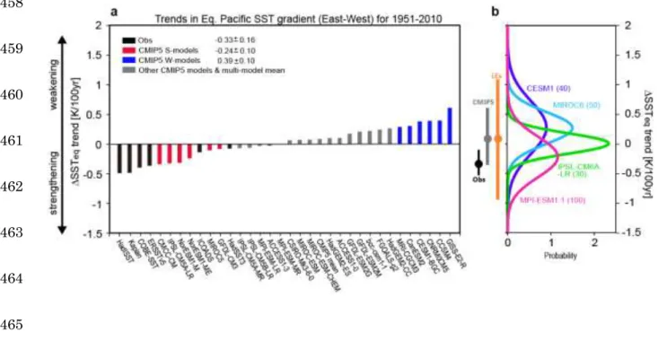
Figure 1 | Linear trends in the equatorial Pacific zonal SST gradient (SSTeq) during 419
1951–2010.
420
a, Trends in six observational data sets (black bars) and 27 CMIP5 models, arranged from
421
strengthening (negative) to weakening (positive)SSTeq. The unit is K per century. Red bars
422
indicate models showing the strengthening of SSTeq consistent with the observations (S-423
models), whereas blue bars indicate models simulating large weakening trend opposite to the
424
observations (W-models). b, Probability density function of SSTeq trends in four large
425
ensemble simulations: CESM1 (blue), IPSL-CM6-LR (green), MPI-ESM1.1 (pink), and
426
MIROC6 (cyan). Numbers in parentheses indicate their ensemble size. Means and the 5–95%
427
ranges for observations, CMIP5 models, and combined LEs are represented, respectively, by
428
black, grey, and orange dots with bars at the left.
429
Figure 2 | Linear trends in the equatorial ocean temperature during 1951–2010.
430
The trend is calculated for the 5°S–5°N strip for a, observations, b, CMIP5 multi-model mean,
431
c, CMIP5 S-model mean, and d, CMIP5 W-model mean. The unit is K per century. The grey
432
shading represents the trend statistically significant at the 95% level. White contours indicate
433
19, 20, and 21 °C isotherms in the climatological states, measuring the depth of mean
434
thermocline.
435
Figure 3 | Linear trends in SSTeq for 50 years with a sliding window between 1951 and 436
2100.
24
a, Ensemble-mean values of the trend from the CMIP5 historical and RCP4.5 simulations by
438
S-models (red), W-models (blue), and all models (grey) represented by squares and dashed
439
curves, with error bars indicating the 66% range. The unit is K per century. The abscissa shows
440
the end year for the 50-year segment. b, Same as a, but for the MPI-ESM1.1 100-member LE,
441
in which ten S- and W-members are selected following the values of SSTeq trend for 1951–
442
2010.
443
Figure 4 | Linear trends in GSAT for 50 years with a sliding window between 1951 and
444
2100.
445
Ensemble-mean values of the trend from the CMIP5 S-models (red curve) and W-models (blue
446
curve) and the 66% range (shading) for a, RCP2.6, b, RCP4.5, and c, RCP8.5 simulations. The
447
abscissa shows the end year for the 50-year segment. The unit is K per century. The linear
448
trends for 1951–2000 are calculated using the historical runs and are highlighted by squares.
449 450 451 452 453 454 455 456 457
25 458 459 460 461 462 463 464 465
Figure 1 | Linear trends in the equatorial Pacific zonal SST gradient (SSTeq) during 466
1951–2010.
467
a, Trends in six observational data sets (black bars) and 27 CMIP5 models, arranged from
468
strengthening (negative) to weakening (positive)SSTeq. The unit is K per century. Red bars 469
indicate models showing the strengthening of SSTeq consistent with the observations (S-470
models), whereas blue bars indicate models simulating large weakening trend opposite to the
471
observations (W-models). b, Probability density function of SSTeq trends in four large 472
ensemble simulations: CESM1 (blue), IPSL-CM6-LR (green), MPI-ESM1.1 (pink), and
473
MIROC6 (cyan). Numbers in parentheses indicate their ensemble size. Means and the 5–95%
474
ranges for observations, CMIP5 models, and combined LEs are represented, respectively, by
475
black, grey, and orange dots with bars at the left.
476 477
26 478 479 480 481 482 483 484 485 486 487
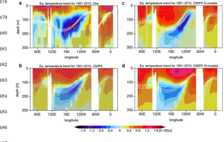
Figure 2 | Linear trends in the equatorial ocean temperature during 1951–2010.
488
The trend is calculated for the 5°S–5°N strip for a, observations, b, CMIP5 multi-model mean,
489
c, CMIP5 S-model mean, and d, CMIP5 W-model mean. The unit is K per century. The grey
490
shading represents the trend statistically significant at the 95% level. White contours indicate
491
19, 20, and 21 °C isotherms in the climatological states, measuring the depth of mean
492 thermocline. 493 494 495 496 497
27 498 499 500 501 502 503 504
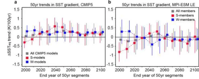
Figure 3 | Linear trends in SSTeq for 50 years with a sliding window between 1951 and 505
2100.
506
a, Ensemble-mean values of the trend from the CMIP5 historical and RCP4.5 simulations by
507
S-models (red), W-models (blue), and all models (grey) represented by squares and dashed
508
curves, with error bars indicating the 66% range. The unit is K per century. The abscissa shows
509
the end year for the 50-year segment. b, Same as a, but for the MPI-ESM1.1 100-member LE,
510
in which ten S- and W-members are selected following the values of SSTeq trend for 1951– 511 2010. 512 513 514 515 516 517
28 518 519 520 521 522
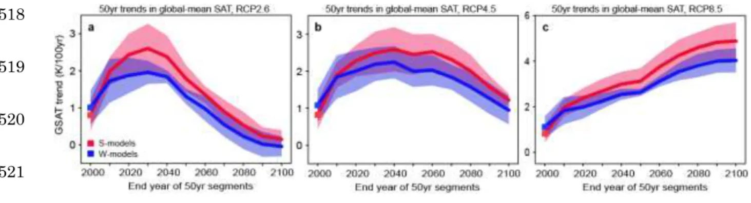
Figure 4 | Linear trends in GSAT for 50 years with a sliding window between 1951 and
523
2100.
524
Ensemble-mean values of the trend from the CMIP5 S-models (red curve) and W-models (blue
525
curve) and the 66% range (shading) for a, RCP2.6, b, RCP4.5, and c, RCP8.5 simulations. The
526
abscissa shows the end year for the 50-year segment. The unit is K per century. The linear
527
trends for 1951–2000 are calculated using the historical runs and are highlighted by squares.
528 529 530 531