Nitrogen oxides emission from two beech forests subjected to different nitrogen loads

HAL Id: hal-00297563

https://hal.archives-ouvertes.fr/hal-00297563

Submitted on 12 Jul 2006

HAL is a multi-disciplinary open access

archive for the deposit and dissemination of

sci-entific research documents, whether they are

pub-lished or not. The documents may come from

teaching and research institutions in France or

abroad, or from public or private research centers.

L’archive ouverte pluridisciplinaire HAL, est

destinée au dépôt et à la diffusion de documents

scientifiques de niveau recherche, publiés ou non,

émanant des établissements d’enseignement et de

recherche français ou étrangers, des laboratoires

publics ou privés.

subjected to different nitrogen loads

B. Kitzler, S. Zechmeister-Boltenstern, C. Holtermann, U. Skiba, K.

Butterbach-Bahl

To cite this version:

B. Kitzler, S. Zechmeister-Boltenstern, C. Holtermann, U. Skiba, K. Butterbach-Bahl. Nitrogen

oxides emission from two beech forests subjected to different nitrogen loads. Biogeosciences, European

Geosciences Union, 2006, 3 (3), pp.293-310. �hal-00297563�

www.biogeosciences.net/3/293/2006/ © Author(s) 2006. This work is licensed under a Creative Commons License.

Biogeosciences

Nitrogen oxides emission from two beech forests subjected to

different nitrogen loads

B. Kitzler1, S. Zechmeister-Boltenstern1, C. Holtermann2, U. Skiba3, and K. Butterbach-Bahl4

1_{Federal Research and Training Centre for Forests, Natural Hazards and Landscape (BFW), Seckendorff-Gudent-Weg 8,}

Vienna, Austria

2_{Sellenyg. 2–4/52, Vienna, Austria}

3_{Institute of Terrestrial Ecology, Bush Estate, Penicuik, Midlothian EH26 OQB, Scotland}

4_{Institute for Meteorology and Climate Research, Atmospheric Environmental Research, Forschungszentrum Karlsruhe,}

Kreuzeckbahnstraße 19, 82467, Garmisch-Partenkirchen, Germany

Received: 1 July 2005 – Published in Biogeosciences Discuss.: 9 September 2005 Revised: 2 May 2006 – Accepted: 8 May 2006 – Published: 12 July 2006

Abstract. We analysed nitrogen oxides (N2O, NO) and

car-bon dioxide (CO2)emissions from two beech forest soils

close to Vienna, Austria, which were exposed to different nitrogen input from the atmosphere. The site Schottenwald

(SW) received 20.2 kg N ha−1y−1and Klausenleopoldsdorf

(KL) 12.6 kg N ha−1y−1through wet deposition. Nitric

ox-ide emissions from soil were measured hourly with an

auto-matic dynamic chamber system. Daily N2O measurements

were carried out by an automatic gas sampling system.

Mea-surements of nitrous oxide (N2O) and CO2emissions were

conducted over larger areas on a biweekly (SW) or monthly (KL) basis by manually operated chambers. We used an au-toregression procedure (time-series analysis) for establishing time-lagged relationships between N-oxides emissions and different climate, soil chemistry and N-deposition data. It was found that changes in soil moisture and soil

tempera-ture significantly effected CO2and N-oxides emissions with

a time lag of up to two weeks and could explain up to 95% of the temporal variations of gas emissions. Event emissions after rain or during freezing and thawing cycles contributed significantly (for NO 50%) to overall N-oxides emissions.

In the two-year period of analysis the annual gaseous N2O

emissions at SW ranged from 0.64 to 0.79 kg N ha−1y−1

and NO emissions were 0.24 to 0.49 kg N ha−1 per

vegeta-tion period. In KL significantly lower annual N2O emissions

(0.52 to 0.65 kg N2O-N kg ha−1y−1)as well as considerably lower NO-emissions were observed. During a three-month measurement campaign NO emissions at KL were 0.02 kg N

ha−1), whereas in the same time period significantly more

NO was emitted in SW (0.32 kg NO-N ha−1_{). Higher}

N-Correspondence to: B. Kitzler (barbara.kitzler@bfw.gv.at)

oxides emissions, especially NO emissions from the high N-input site (SW) may indicate that atmospheric deposition has an impact on emissions of gaseous N from our forest soils. At KL there was a strong correlation between N-deposition and N-emission over time, which shows that low N-input sites are especially responsive to increasing N-inputs.

1 Introduction

Nitrogen emissions are driven by soil substrate, tree species, climate, short term fluctuations of water availability as high rain, freeze thaw cycles and atmospheric inputs (e.g. Dahlgren and Singer, 1994; Fitzhugh et al., 2001; Lovett et al., 2002; MacDonald et al., 2002). The effect of N-deposition on N-emissions has become a major issue due to the observation of a significant worldwide increase in N-deposition rates; a further increase is predicted as a result of an increased use of fertilizers and increased energy con-sumption (Galloway et al., 1995; Hall and Matson, 1999). In forest ecosystems increased N supply results in N saturation which is indicated by increased N-leaching from soils, soil acidification, forest decline, nutrient imbalances and losses, and soil emissions of N oxide gases (Gundersen et al., 1998; van Breemen et al., 1988; Aber et al., 1998; Skiba et al., 1999). Where N constitutes a limiting factor, competition

between roots and microbes is high and nitrate (NO−₃) is

taken up. This is contrary to a high N supply which leaves

ammonium (NH+₄) and NO−₃ accessible for nitrifying and

denitrifying bacteria. Chemodenitrification, nitrification and denitrification are the main sources of N-oxides emissions (Davidson, 1993; Venterea et al., 2003). Forest ecosystems

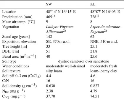
Table 1. Site and soil characteristics of the investigation sites Schottenwald and Klausenleopoldsdorf.

SW KL

Location 48◦140N 16◦150E 48◦070N 16◦030E Precipitation [mm] 4651) 7281)

Mean air temp. [◦C] 9 8

Vegetation Lathyro-Fagetum Asperulo odoratae-Allietosum2) Fagetum2)

Stand age [years] 142 62

Exposition, elevation SE, 370 m a.s.l. NNE, 510 m a.s.l. Tree height [m] 33 25.1

DBH [cm] 51 21.8

Basal area [m2ha−1] 40 25.6 Soil type dystric cambisol over sandstone Water conditions moderately well-drained moderately fresh Soil texture silty loam loam-loamy clay Soil pH 0–7 cm (CaCl2) 4.4 4.6

C:N 16 16

Soil density (g cm−3) 0.630 0.827 Ntot(mg g−1) 2.38 4.79

Corg(mg g−1) 37.70 74.51 1)_{Mean precipitation of the two observation years.}

2)_{Mayer (1974).}

with N-inputs exceeding critical loads have been found to accumulate N in soil (Beier et al., 2001). However, studies in N-saturated forests in Central (Zechmeister-Boltenstern et al., 2002; Butterbach-Bahl et al., 1997; Brumme and Beese, 1992) and Northern Europe (Pilegaard et al., 1999) have shown that N-saturated forests release significantly more

N2O and, especially NO, than N-limited temperate forests

(Davidson and Kingerlee, 1997).

In the vicinity of cities or intensively managed agricultural

lands, N-input can amount up to 50 kg N ha−1y−1(NADP,

2002; Tietema, 1993). Since there are only a few

stud-ies that investigated the effect of different N-deposition on forest ecosystems under similar climatic conditions (Hahn et al., 2000; Rennenberg et al., 1998; Skiba et al., 1998; Butterbach-Bahl et al., 2002a) our approach included: (1)

Field measurements of CO2, N2O and NO emissions from

soils of two beech forests with different N-deposition loads. Additionally, measurements were made in high temporal and spatial resolution to (2) get better estimates of annual emis-sion (3) study the effects of climatic factors and soil param-eters on gaseous soil emissions and (4) find an appropriate statistical procedure to describe the relationships between N-emissions and their ecological drivers.

2 Material and methods

2.1 Investigation sites and soils

The experimental site Schottenwald (SW) is situated in direct vicinity of Vienna on a SE-exposed upper slope in a 142 year old beech stand. The soil is a moderately well drained dys-tric cambisol over sandstone. In spring the undergrowth is dominated by a dense cover of the geophyte Allium ursinum L. changing to bare soil in summer and autumn. The second sampling site, Klausenleopoldsdorf (KL), is located about 40 km south-west of Vienna on a NNE-facing slope. On site there is a 62 year old beech forest growing on a dystric cam-bisol displaying no significant changes in ground vegetation throughout the year. For site description see Table 1.

2.2 N2O and CO2flux measurements

We used the closed chamber technique in order to cover the

spatial and temporal variability of N2O and CO2soil

emis-sions. Gas emissions were measured by manual (4/site) and automatic chambers (1/site). A manual chamber consists of an aluminium frame (1×1×0.05 m), which we inserted into the soil to a depth of 3 cm. A single-wall rigid polyethylene light-dome (Volume: 80 l) with a compressible PTFE seal at the bottom was fixed onto the aluminium frame by means of 4 screws.

Duplicate air samples were taken from the chambers with 60 ml polypropylene gas-tight syringes at an interval of 0, 1 and 2 h.

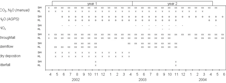
Fig. 1. Measurement frequency of CO2and N2O emissions by manual chambers, N2O emissions by AGPS, NOxby dynamic chambers,

litterfall and depositon data at Schottenwald and Klausenleopoldsdorf. (x)=1/month, (xx)=2/month, (o)=1/day, (-)=1/h.

Linearity of emission was always tested. We never

ob-served a flattening of the N2O increase in our chambers,

which would indicate that we approached the compensation

point for N2O. Additional measurements every 15 minutes

showed that the increase in N2O concentrations remained

lin-ear for up to 4 hours (Zechmeister-Boltenstern et al., 2002). 30 ml of the gas-probe were injected into evacuated and gas tight headspace vials (20 ml), fitted with a silicon sealed rubber stopper and an aluminium cap. Samples were taken on a biweekly (SW) or monthly (KL) basis from April 2002 until May 2004 (Fig. 1).

For the measurement of short-time temporal variations

(1/day) (Fig. 1) of N2O emissions an automatic gas sampling

system (AGPS-patent DE 198 52 859) was used (UIT GmbH,

Dresden). It consists of the following main components

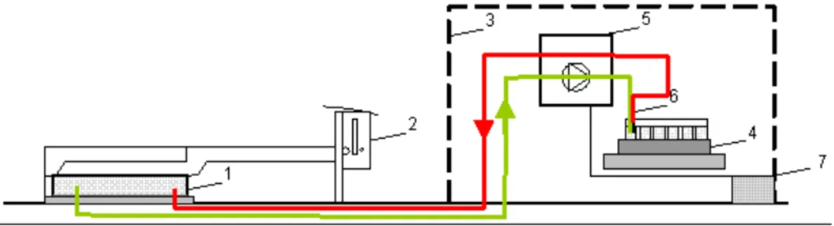
(Fig. 2): A covering case (0.7×0.7 m) with a rubber gasket, a slipping clutch for automatically closing and opening of the chamber and a thermostat. Within the protection case a fraction collector with 40 headspace vials (20 ml), a control system; a vacuum pump and a memory programmable con-trol unit with the possibility of the free determination of the sampling times; an automatic needle plug-in with a double needle; the power supply that is provided either by batteries (2×12 V/DC) (at KL) or by existing power supply lines (at SW) where a mains adapter EP-925 (230 V to 24 V/DC) was interposed.

During sampling procedure the covering case glided across to the side of the sealing plate, thus, case-tightening the chamber for 70 min. During closure time air samples

were extracted (flow rate ca. 100 ml min−1) from the

cham-ber by a membrane pump and transported through 10 m Teflon tubes to the vials. Sample lines and vials were flushed for 10 min before samples were taken from the headspace air of the chamber. Within these 70 min two gas samples were taken: The first one after 10 min, the second one after 70 min

closure time. Automatic sampling was scheduled for 6 a.m. During winter time measurements took place at 1 p.m., thus, avoiding night/morning frost. In order to prevent the cov-ering case from freezing on the sealing plate the thermostat

was set at 1◦C and no measurements were conducted below

this temperature.

The vials with the gas samples were stored at 4◦C

un-der water for 14 days maximum. In the laboratory gas

samples were analysed for N2O by gas chromatography

(HP 5890 Series II) with a 63Ni-electron-capture detector

(ECD) connected to an automatic sample-injection system (DANI HSS 86.50, HEADSPACE-SAMPLER). Oven,

injec-tor and detecinjec-tor temperatures were set at 120◦C, 120◦C and

330◦_{C, respectively. N}

2 in ECD-quality served as

carrier-gas with a flow rate of 30 ml min−1_{. The gas-chromatograph}

was routinely cross-calibrated with a standard of 5 µl l−1

N2O (Linde Gas) and dilution series were made

regu-larly. We quantified a minimum detectable N2O flux of

0.04 µg N m−2h−1and the relative error falls below <17%

with a median of 5%. CO2was analysed through a gas

chro-matograph (Hewlett-Packard 5890 II series) equipped with a thermal conductivity detector (TCD). Helium was used as carrier-gas (flow rate 10 ml min−1); the CO2 standard

con-tained 10 ml l−1CO2(Linde Gas). The minimum detectable

CO2flux was 0.001 mg C m−2h−1.

Emissions of N2O (µg N m−2h−1)and CO2 (mg C m−2

h−1)were determined by the linear increase of the mixing

ratio within the headspace of the closed chamber. The

cal-culation of N2O and CO2fluxes is described in the manual

on measurement of CH4and N2O emissions from agriculture

(IAEA, 1992).

2.3 NO flux measurements

NO and NOx exchange was directly measured on site

Fig. 2. Schematic of the AGPS with the main components 1) covering case; 2) slipping clutch and a thermostat; 3) protection case; 4) fraction

collector; 5) control system, vacuum pump and memory programmable control unit; 6) double needle and 7) power supply.

detection limit of the NOx-analyzer (HORIBA APNA-360)

was 1 ppbv NO. The detection limit of the dynamic

cham-ber system is 0.6 µg NO m−2_h−1_{. The reading for NO}

x of

the HORIBA analyzer refers to NO, NO2 and other

nitro-gen compounds (PAN, NH3, HONO, HNO3, aerosol

ammo-nium, nitrate and nitrite). We therefore use the terms NO

and (NOx-NO) further on. The calculated error was high

for fluxes near the detection limit (∼130%), whereas it was low for high NO fluxes (∼3%). A median error was

cal-culated to be ∼15% and ∼35% for NO and (NOx-NO),

re-spectively. Air samples were taken from six stainless steel chambers (Area: 0.03 m2; Vol: 3.27 l; flow rate: 1 l min−1)

connected to the NOx-analyzer via PTFE tubing (inner

di-ameter: 4 mm; length: 10 m). The closing (Plexiglas lid) of the dynamic chambers is initiated by a motor. One of the six dynamic chambers was used as a reference chamber by sealing the opening to the soil through a Plexiglas pane. The chambers were closed for 5 min within which steady state was reached. Since there was no ozone analyzer available in 2002, the chamber inlets were supplied with clean air. For this ambient air was passed through a filter cylinder filled with Purafil and activated charcoal (length: 465 mm; diam-eter: 85 mm). Calibration was carried out through span gas (UBA certified) of a NO concentration of 153±2% ppb. Zero air preparation consisted of a bottle of compressed synthetic

air (Cn Hm<0,1 vpm and NOx<0,1 vpm). Considering the

basically bi-directional nature of NO exchange, the opera-tion of dynamic chambers under “zero-gas” condiopera-tions (NO free air) can lead to an overestimation of NO fluxes due to exposing the enclosed soil to low NO concentrations (Lud-wig et al. 2001). As the NO fluxes measured from our cham-bers are very low and NO concentrations are under calculated compensation points of 50 ppbv (SW) and 24 ppbv (KL) (at

15◦C) determined in a laboratory experiment the error using

“zero-gas” was neglible in our case.

In 2002, the flux rate of NO was calculated based on the equation described in Schindlbacher et al. (2004). In year

2003, both, NO, (NOx-NO) concentrations and O3

concen-trations (HORIBA APOA-360) were measured in the cham-ber atmosphere without using a filter. Nitric oxide and (NOx -NO) fluxes were calculated as described in Butterbach-Bahl

et al. (1997), thus, taking the chemical reaction occurring

between O3and NO in the chambers and in the tubing into

account (Eq. 1). F = Q · (mNOmc−mNOrc) ·MN·60 · 10 6 Vm·A ·109 mNOmc=k3·mNOt·mO3t·tmc+mNOt mNOt= (mO3−mNO)mNO mO3·10(−k3·(mO3−mNO)·tt)−mNO mO3t= (mNO−mO3)mO3 mNO · 10(−k3·(mNO−mO3)·tt)−mO3 (1)

Where F is the flux rate [µg N m−2h−1], Q is the mass

flow rate of air through the chamber (∼0.001 m3min−1),

mNOmc=corrected mixing ratio for NO in the measuring

chamber [ppbv], mNOrc=corrected mixing ratio of NO in

the reference chamber, MN is the atomic weight of N

(=14.0067 g mol−1), Vmis the standard gaseous molar

vol-ume (24.055·10−3m3mol−1), and A is the soil surface

area of the chamber (0.0314 m2), k3=1,8 10−12 e(1370/T ) [cm3molecule−1s−1] or 4,8 10−2e(1370/T )[ppbv−1min−1],

mNOt=corrected mixing ratio for NO at the beginning of the

tubing system [ppbv], mO3t=corrected mixing ratio for O3at

the beginning of the tubing system [ppbv], tmcresidence time

of sample air in the measuring chamber [s], mNO=mixing

ratio detected by the NO-analyzer [ppbv], mO3=mixing

ra-tio of O3detected by the O3-analyzer [ppbv], T =temperature [K], tt=residence time of sample air in the tubing [s].

(NOx-NO) was calculated in analogy to NO flux rates

(Butterbach-Bahl et al., 1997) using the (NOx-NO)-converter

efficiency that was determined at the UBA, Vienna.

In our calculations we have not considered losses of NO,

(NOx-NO) or O3to the chamber walls, since a previous study

by Ludwig (1994) showed that e.g. deposition of NOx to

the chamber walls may in maximum contribute <20% to

the total deposition flux even if the NOxmixing ratio within

the chamber was >15 ppbv. In view of the low

concentra-tions and the spatial heterogeneity of NOxfluxes the

assumed to be of minor importance. An error analyses

re-vealed that O3loss to chamber walls is not a source of

con-cern. If O3would be lost by as much as 30%, as reported by

Ludwig (1994) for full Perspex chambers, the change of NO flux is less than 0.2 µg N m−2h−1which is smaller than the detection limit.

2.4 Soil samples

Around the chambers square plots of 4×4 m2were marked.

Every 2 months samples of the organic layer (frame 30×30 cm) and mineral soil (metal cylinder with 5 cm height, 7 cm diameter) were taken from the corners of each plot, moving clockwise in order to avoid re-sampling at the

same spot. No soil samples were taken during times of

snow cover. Four soil samples of each plot were pooled and sieved through a 2-mm sieve. Litter samples were pooled and ground. Soil and litter samples were analysed for ex-tractable NH+₄-N and NO−₃-N concentrations, soil moisture

and pH. Ammonium and NO−₃ were extracted from soil with

0.1 M KCl. Ammonium was determined by a modified in-dophenol reaction (Kandeler, 1995). Nitrate was measured

as NO−₂-N after reduction by copper sheathed zinc

granu-lates. Values are reported in µg N g−1soil dry weight (dw).

Soil moisture was determined gravimetrically and the pH

was measured in soil suspensions in 0.01 M CaCl2solution

using a glass electrode.

2.5 Meteorological data

Air temperature (◦C) and relative humidity (%) were

mea-sured with a combined temperature moisture sensor at 2 m above ground. Daily precipitation was taken from the near-est meteorological stations in Mariabrunn (2.7 km from SW) and in Alland (7 km from KL). Soil temperature was mea-sured by thermocouples; and soil water content by a water content reflectometer (CS615) at a soil depth of 5 cm, 15 cm and 30 cm in SW and 15 cm, 30 cm and 60 cm in KL. Data were stored at an interval of 0.5 h in the data logger (Delta-T Logger).

2.6 Deposition measurements

Wet deposition was collected biweekly using 10 and 15 throughfall collectors, and 2 and 3 stemflow collectors at SW and KL, respectively. Litterfall was collected in three collectors. Wet deposition and litterfall was analysed for

NH+₄-N and NO−₃-N. Dry deposition as one component of

the N budget comprises NH3and NO2, but also dry

deposi-tion of NO (if soil compensadeposi-tion mixing ratio is exceeded),

HONO, HNO3, PAN, aerosol ammonium, nitrate and

ni-trite. In this study concentrations of nitrogen dioxide (NO2)

and ammonia (NH3)was measured by three passive

diffu-sion tubes and three CEH ALPHA samplers (Tang, 2001) and were analysed by CEH Edinburgh. Passive diffusion

samplers are widely used to monitor atmospheric

concen-trations of trace gases such as NH3 and NO2 (Krupa and

Legge, 2000; Brown, 2000). The ammonia ALPHA sam-pler method (used by CEH, Edinburgh) was rigorously tested against a reference active diffusion denuder method (Sutton et al., 2001). A modification of the GRADKO diffusion tube,

which is widely used in the UK was used for monitoring NO2

(Stevenson et al., 2001). This diffusion tube was modified by adding a turbulence damping membrane across the inlet and validated by Bush et al. (2001). The samplers were placed at a height of 1.5 m in the canopy at the forest sites and were changed monthly. In order to estimate the rates of dry depo-sition, deposition velocities of 1.5 mm s−1for NO2and 3 mm

s−1for NH3(Duyzer, pers. comm.) were assumed.

Concen-trations of NO2and NH3were measured in the first

investi-gation year (May 2002–April 2003), whereas wet deposition was measured in the first and the second ( May 2003– April 2004) investigation year (Fig. 1).

2.7 Statistical analysis

Differences in soil emission, soil chemistry data and N-deposition data between the sites and between the investi-gation years were determined using the t-test or the nonpara-metric Wilcoxon-test. Prior to analysis the data were checked for normal distribution and for homogeneity of variances (t-test). When normal distribution could not be achieved by log-transformation, the Wilcoxon-test was carried out. The relationships between daily, biweekly or monthly fluxes and soil, meteorological or deposition data were investigated us-ing Pearson Correlation or Spearman rank correlation.

Soil emissions, soil, and meteorological data were serially correlated over time. We therefore used an autoregression procedure that provides regression models for time series data when the errors are autocorrelated or heteroscedastic. Data are said to be heteroscedastic (non-constant) if the vari-ance of errors is not steady. As one of the key assumptions of the simple linear regression model is that the errors have the same variance throughout a sample the regression model

has to correct for heteroscedasticity. We therefore used

the generalized autoregressive conditional heteroscedastic-ity (GARCH) model to correct for heteroscedasticheteroscedastic-ity. The GARCH (p, q) process assumes that the errors, although uncorrelated, are not independent and it models the time-varying conditional error variance as a function of the past realizations of the series (SAS/ETS, 1993). Models that take the changing variance into account can explore data more ef-ficiently. The basic autoregressive conditional heteroscedas-ticity ARCH(q) model is the same as the GARCH(0,q) model, where (p) references about the number of autore-gressive lags and (q) references about the number of mov-ing average lags. The stepwise autoregressive error model was used for correcting autocorrelation. First, this method fits a high-order model with many autoregressive lags and then removes autoregressive parameters sequentially until

Table 2. Wet and dry deposition and litter-fall [kg N ha−1y−1], precipitation [mm], soil nitrogen [µg N g−1dw] and pH (CaCl2) in year 1

(May 2002–April 2003) and year 2 (May 2003–April 2004) at the two investigation sites Schottenwald and Klausenleopoldsdorf.

SW KL

year 1 year 2 year 1 year 2 N-input by wet deposition [kg N ha−1y−1]

throughfall NH+₄-N 8.6 4.8 5.5 2.5

NO−₃-N 7.7 9.9 6.0 2.5

stemflow NH+₄-N 2.71) 2.6 0.6 0.4

NO−₃-N 1.21) 2.1 0.5 0.3

Sum of wet deposition 20.2 19.4 12.6 5.7

N-input by dry deposition [kg N ha−1y−1]

NH3-N 1.08 n.m. 0.23 n.m.

NO2-N 1.30 n.m. 0.62 n.m.

Sum of dry deposition 2.38 n.m. 0.85 n.m.

Precipitation [mm] 530 400 765 690 Litter-fall [kg dw ha−1y−1] 4030 (177) 5963 (920) 6840 n.m. N – litterfall [kg N ha−1y−1] 52.8 (3.7) 74.5 (10.6) 59.2 n.m. Organic layer [µg N g−1dw] NH+₄-N 97.6 (9.4) ** 55.0 (5.6) ** 50.0 (4.3) 25.5 (1.5) NO−₃-N 19.5 (1.8) ** 27.5 (2.8) * 11.4 (1.2) 18.0 (2.3) pH (CaCl₂) 5.7 (0.1) * 5.7 (0.1) * 5.4 (0.1) 5.2 (0.1) Mineral soil [µg N g−1dw] NH+₄-N 9.4 (1.4) 4.0 (0.4) 11.5 (1) * 5.7 (0.5) NO−₃-N 1.5 (0.3) *** 1.7 (0.2) * 0.4 (0.1) 0.9 (0.1) pH (CaCl2) 4.4 (0.1) 4.3 (0.04) 4.6 (0.1) 4.6 (0.04)

Note: Deposition data and precipitation are sums. Soil data are means with standard error in parenthesis.

1)_{Starting from August 2002. Asterisks indicate significant differences between the sites for the individual years (* p<0.05, ** p<0.01,}

*** p<0.001). n.m. = not measured.

all remaining autoregressive parameters display significant t-tests. With this model the most significant results can be detected. The basic equation for the autoregression model used is as follows (Eq. 2):

yt =β0+β1x1t+β2x2t+. . . βnxnt +vt vt =εt−ϕ1vt −1−ϕ2vt −2−. . . − ϕmvt −m εt = p htet ht =ω + q X i=1 αiεt −i2 + p X j =1 γjht −j et ∼I N (0, 1) (2)

where yt is the dependent variable for time t, β0is the inter-cept; β1, β2, . . .βn are the regression coefficients of the in-dependent variables (xit, i=1. . .n) where x1tis soil moisture

in 15 cm (SW) and 30 cm (KL) soil depth, x2t is soil

tem-perature in 3 cm (for N2O), 5 cm (for NO) (SW) and 5 cm

(KL) soil depth and x3t is the CO2 emission rate. vt is the

error term that is generated by the j th order autoregressive

process; ϕm are the autoregressive error model parameters

(ARm). The order of the process (m) defines the number of

past observations on which the current observation depends;

εt is the unconditional variance and ht is the GARCH (p, q)

conditional variance; etis assumed to have a standard normal

distribution; the parameters (ω and α1) are ARCH (q) model

estimates and (γ1) are GARCH (p) model estimates.

Statisti-cal analysis was either completed with SAS Enterpriseguide Version 2 or SAS Version 8. All differences reported were significant at p<0.05 unless otherwise stated.

3 Results

3.1 Meteorological data

The two years were characterized by extreme weather condi-tions. In summer/autumn 2002 disastrous flooding occurred all over Europe because of persistent rainfall, followed by an extensive drought period in summer 2003. Consequently, the differences between the two seasons were pronounced, particularly in terms of soil moisture content. During both years significantly (p<0.001) lower mean soil moisture was recorded in SW (28% and 19%) in comparison to KL (42%

and 37%). Mean annual air temperature was 8.0 and 8.2◦C

at SW and KL, respectively. In the second year higher mean

Fig. 3. Extractable soil nitrogen (NH+₄-N and NO−₃-N) in the litter layer (circles) and in the mineral soil (0–5 cm) (triangles), at Schottenwald and at Klausenleopoldsdorf. Pooled samples (n=4) were taken from around the individual chambers.

Fig. 4. Bar chart: Monthly N-input (kg N ha−1)and precipitation [mm] at Schottenwald and Klausenleopoldsdorf for the years 2002–2004.

Pie charts: Portion of throughfall (TF NH+₄-N, TF NO−₃-N), stem-flow (stem NH₄+-N and stem NO−₃-N) on annual N-input (kg N ha−1)in the first investigation year (May 2002–April 2003).

3.2 Soil nitrogen

At both sites NH+₄-N concentrations in mineral soil reached

highest levels with concentrations of up to 17.3 µg NH+₄

-N g−1dw in SW and 17.9 µg NH+₄-N g−1 dw in KL in

September 2002. In the first year mean NH+₄-N

concentra-tions were considerably higher compared to the quantified

concentrations in the second year (Table 2), whereas NO−₃

-N concentrations were higher in the second year. The soil

in SW displayed highest NO−₃-N concentrations in summer

(max: 3.4 µg NO−₃-N g−1dw) when Allium leaves had

de-cayed completely and in autumn after litterfall (max: 2.3 µg

NO−₃-N g−1 dw). The soil in KL showed highest NO−₃-N

concentrations from August to October 2003 (up to 1.3 µg NO−₃-N g−1dw).

Total extractable soil N (NO−₃-N and NH+₄-N) concentra-tions were found to be significantly (p<0.001) higher at both

sites in the first year of investigation. Concentrations of

avail-able NO−₃-N and NH+₄-N in the organic layer were about

twice as large in soil samples from SW in comparison to KL but similar in terms of mineral soil (Fig. 3).

3.3 Nitrogen input

Nitrogen input by wet (NO−₃-N and NH+₄-N) and dry

deposi-tion (NH3-N and NO2-N), litter decomposition and

mineral-ized N are demonstrated in Table 2 and Fig. 4. Nitrogen input through litterfall to the forest floor amounted to 53–75 kg N per ha−1y−1at SW, whereas in KL N-input through litterfall amounted to 59 kg N per ha−1y−1.

Differences between the sites regarding the stem-flow of N were significant (p<0.05) in both years; differences in N from throughfall were significant in the second year.

Con-centration of NH3, NO2 was measured in the first year

µg N 2 O-N m -2 h -1 0 10 20 30 40 50 2002 2003 2004

M ay Jul Sep N ov Jan M ar M ay Jul Sep N ov Jan M ar M ay

soil m o isture [c m 3 cm -3] 0 20 40 60 p reci p itation [mm ] 0 10 20 30 40 50 mg C O 2 -C m -2 h -1 0 50 100 150 soil te m p erature [° C ] -5 0 5 10 15 20 b) c) a)

Fig. 5. (a) Mean CO2emissions (squares±S.E) measured with the manual chambers and soil temperature [5 cm] (black line), (b) mean

N2O emissions from manual (circles±S.E) and automatic (diamonds) chambers and (c) daily precipitation (at Mariabrunn) and soil moisture

[15 cm] at the site Schottenwald from April 2002 to June 2004.

µg N 2 O-N m -2 h -1 0 10 20 30 40 50 2002 2003 2004 May Jul Sep Nov Jan Mar May Jul Sep Nov Jan Mar May

soil moisture [c m 3 cm -3] 0 20 40 60 p reci p itation [mm ] 0 10 20 30 40 50 mg CO 2 -C m -2 h -1 0 50 100 150 soil temperature [°C] -5 0 5 10 15 20 25 b) c) a)

Fig. 6. (a) Mean CO2emissions (squares±S.E) measured with the manual chambers and soil temperature [5 cm] (black line), (b) mean N2O

emissions from manual (circles±S.E) and automatic (diamonds) chambers and (c) daily precipitation (at Alland) and soil moisture [15 cm] at the site Klausenleopoldsdorf from May 2002 to May 2004.

54.2 µg NO2 m−3 in SW and KL, respectively. Under the

assumption that the above mentioned deposition velocities

are correct we estimated a depostion of NH3 and NO2 of

2.38 and 0.85 kg N ha−1 y−1 in SW and KL, respectively,

thus, displaying highly significant differences between the

sites (p<0.001). A total of 20.2 kg and 12.6 kg N ha−1y−1 were deposited via wet deposition in SW and KL, respec-tively (year 1) and it has to be emphasized that N-deposition is dominated by wet deposition at our sites.

3.4 Gas fluxes

3.4.1 CO2emissions

CO2fluxes are shown in Figs. 5a and 6a. The annual mean

of CO2 emissions varied between 33.0 and 43.4 mg CO2

-C m−2 h−1 at SW and between 29.2 and 31.6 mg CO2-C

m−2h−1 at KL, respectively (Table 3). Significant

differ-ences (p<0.05) between the sites were observed mainly dur-ing sprdur-ing and autumn, whereas in summer and winter soil

CO2fluxes did not differ remarkably between the sites. The

fluxes showed clear seasonal variations which were strongly

related to the air temperature. Maximum mean CO2 fluxes

were measured in summer 2002 (Figs. 5b, 6b). Lower emis-sion rates (<70 mg CO2-C m−2h−1)were observed during

the dry summer 2003. At SW a second emission peak

could be observed in September, which is probably due to the decomposition of fresh litterfall. At both sites lowest

CO2 emission rates were measured in December. In SW

2.9 t C ha−1_y−1_{were emitted in the two years whereas in KL} total gaseous C-emissions from soil averaged 2.4 t C ha−1_y−1 (Table 4). A correlation analysis showed that 76% and 89%

of variances in CO2 emissions at SW and KL could be

ex-plained by soil temperature (p<0.001). Furthermore, CO2

emissions were negatively correlated with soil moisture in

the upper 15 and 30 cm soil depth (SW: r2=−0.55 and KL:

r2=−0.40).

3.4.2 N2O emissions

At both sites N2O emissions showed a comparable seasonal

trend (Figs. 5b and 6b) with highest rates in summer and in late autumn.

At SW mean annual N2O fluxes amounted to 10.4±0.6 µg

N2O-N m−2h−1in the first year of investigation. Maximum

emissions occurred in July 2002 (75.4 µg N2O-N m−2h−1)

and minimum emission rates in winter 2002 (−6.3 µg N2

O-N m−2 h−1). Nitrous oxide fluxes of up to 39 µg N2O-N

m−2h−1were observed during winter 2002 and reached

al-most the same magnitude as the peaks in spring and autumn. These high winter fluxes were observed during a period of warm weather and in connection with the thawing of the soil. Nitrous oxide fluxes measured in KL were generally lower than those measured in SW (Table 5) except for measure-ments in April 2002 (39.2 µg N2O-N m−2h−1), i.e. at the beginning of the measurements. This might be due to thin-ning of the stand in the previous winter. The annual mean N2O flux was 6.8±0.5 µg N2O-N m−2h−1in the first year

with a minimum of −1.0 µg N2O-N m−2h−1in December

and a maximum of 82.8 µg N2O-N m−2h−1in September.

The mean annual N2O emissions were higher in the second

year (7.6±0.5 µg N2O-N m−2h−1)(Table 3).

The variation coefficient between the manual chambers ranged from 20% to 180% with highest variations in winter 2002 and in summer 2003. lnN 2 O [µg N m -2 h -1] 1 2 3 4 5 2002 2003 2004

Apr Aug Dec Apr Aug Dec Apr

1 2 3 4 r² = 0.53 (a) r² = 0.73 (b)

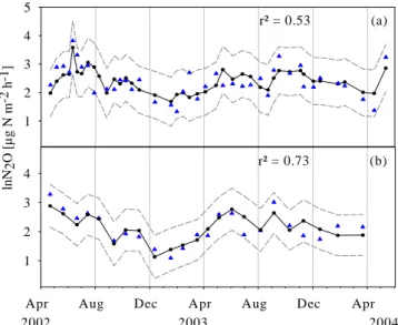
Fig. 7. Measured (triangles), predicted (line with circles) and

con-fidence limits (dashed lines) for log-transformed N₂O emissions in Schottenwald (a) (Model 1) and Klausenleopoldsdorf (b) (Model 2) over the investigation years. Independent variables are soil mois-ture, soil temperature and CO2emission for both sites.

Autoregres-sive parameters are shown in Table 6.

Log-transformed N2O emission rates measured by the

manual chambers were positively correlated (SW: r2=0.54,

KL: r2=0.56, p<0.001) with CO2 emission rates and soil

temperature (r2=0.29, r2=0.40, p<0.001). A significant

positive dependency was found between soil N2O

emis-sions at SW and NO−₃-N concentrations in the organic layer

(r2=0.43, p<0.01). There was no significant correlation be-tween N2O fluxes and soil extractable N (NH+₄-N and NO−₃ -N) in KL.

Soil and meteorological parameters correlated with daily fluxes measured by AGPS as follows: Significant corre-lations (Pearson correlation coefficients) were detected

be-tween daily log-transformed N2O and NO fluxes (r2=0.23;

p<0.001; n=289) in SW, while at KL a significant positive relationship with soil temperature (p<0.01; r2=0.16; n=330) was demonstrated.

A GARCH (1,1) model was developed to predict mean

log-transformed N2O emissions from soil, in SW (Model 1;

r2=0.53) and in KL (Model 2; r2=0.73) (Figs. 7a, b).

Es-timated parameters are shown in Table 6. Due to the fact, that CO2emission rates are significantly correlated with N2O emissions, and soil moisture as well as soil temperature have

a strong effect on N2O emissions these variables were used

within the GARCH model. Furthermore these variables were

measured regularly and simultaneously with N2O emissions

from the manual chambers. For model 1 soil temperature was squared for removing negative values. Model 1 revealed

a time-lag of 14, which means that actual N2O emissions

Table 3. Mean annual CO2-C [mg C m−2h−1], N2O-N and NO-N [µg N m−2h−1] emissions±S.E at Schottenwald and Klausenleopoldsdorf

in the two investigation years (year 1: May 2002–April 2003 and year 2: May 2003–April 2004). Minimum and maximum values are in parenthesis. SW KL CO₂ N₂O NO CO₂ N₂O NO [mg C m−2h−1] [µg N m−2h−1] [mg C m−2h−1] [µg N m−2h−1] year 1 43.41±4.1 10.42±0.6 3.57±0.1 31.57±4.0 6.82±0.5 (0.7–177.5) (−6.3–75.4) (1.2–5.7) (0.9–82.8) (−1.0–48.6) year 2 33.00±2.9 10.15±0.4 7.36±0.6 29.23±3.2 7.63±0.5 0.671)±0.1 (0.2–103.4) (0–41.8) (0.2–44.9) (2.9–77.6) (0.03–37.4) (0–2.2)

1)_{Total NO-N emission between August and October 2003.}

Table 4. Total measured versus total predicted (bold type) CO2-C, N2O-N (manual chambers) and NO-N emissions (±S. E) at Schottenwald

and Klausenleopoldsdorf in the two investigation years (year 1: May 2002–April 2003 and year 2: May 2003–April 2004). Predicted values are based on Models 1 to 4.

SW KL CO₂ N₂O NO CO₂ N₂O NO [kg C ha−1y−1] [kg N ha−1y−1] [kg C ha−1y−1] [kg N ha−1y−1] year 1 2916 ±491 0.79 ±0.004 0.24 ±0.004 2413 ±230 0.64 0.014 0.75 ±0.003 0.18 ±0.005 0.54 ±0.031 0.026 ±0.002 year 2 2875 ±430 0.79 ±0.006 0.49 ±0.038 2315 ±281 0.65 ±0.010 0.0211) ±0.001 0.82 ±0.005 0.39 ±0.022 0.67 ±0.021 0.018 ±0.001

1)_{Total NO-N emission between August and October 2003.}

emission over a period of 14 days. For model 2 (KL) mean

CO2 emissions (x3) were log–transformed. As in KL

mea-surements were carried out once a month we could not detect a similar lag at this site as time between the samplings was too large. By applying the GARCH (1,1) model and hence the calculation of an autoregressive error term, significant ef-fects of variables could be detected that had not been visible before (Table 6).

3.4.3 NO emissions

In SW the NO fluxes from soil were measured from June

2002 until May 2004 (Fig. 8a). During winter no flux

measurements were carried out. Mean NO emission rates

were 3.6±0.1 µg NO-N m−2 h−1 in the first year (June–

November 2002; n=114) with no significant differences

be-tween monthly means. In the second year (May 2003–

January 2004; n=195) significantly higher emission rates

were measured with a mean of 7.4±0.6 µg NO-N m−2h−1

(Table 3). In this year the variation of NO fluxes between the chambers was higher compared to the fluxes measured in the first year.

Highest NO emissions were measured in September after a rainfall event (35 mm), which occurred after an extended dry

period at low soil moisture contents (7–17%) and at soil

tem-peratures between 10 and 15◦_{C. (NO}

x-NO) was deposited

(year 2) with a mean of −2.7±0.09 µg N m−2_h−1_{. Only in}

July the soil seemed to act as a weak net source of (NOx

-NO).

To quantify soil NOx fluxes at KL measuring

cam-paigns were carried out between August and October 2003. The mean NO fluxes measured in this period were

0.7±0.1 µg NO-N m−2h−1 in KL, whereas for the same

period of time, significantly (p<0.001) higher NO fluxes

(Fig. 8b) with a mean of 10.4±1.3 µg N m−2h−1 (−0.8 to

44.9 µg N m−2h−1)were detected at SW. At KL a weaker

deposition of (NOx-NO) was observed with a mean of

−0.6±0.06 µg N m−2h−1.

Daily variations in NO emission could partly be ex-plained by changes in soil temperature at a depth of 5– 30 cm (r2=0.23, p<0.001), and by air temperature (r2=0.17,

p<0.01), respectively. NO and N2O emissions were posi-tively correlated (r2=0.23, p<0.001) in SW. A simple regres-sion model could not be developed to identify relationships between NO emissions and other parameters because resid-uals were correlated over time. An autoregression model (Model 3) was developed, where soil moisture at 15 cm soil

Table 5. Monthly mean N2O and NO emissions in µg N m−2h−1 derived from (a) manual chambers (in Schottenwald-biweekly, in

Klausenleopoldsdorf-monthly) and (b) AGPS system (1/day) and the continuous dynamic system (c).

SW KL N2O NO N2O NO (a) (b) (c) (a) (b) (c) Apr-02 7.65 24.59 * May-02 16.37 14.17 Jun-02 27.53 * 18.40 3.13 9.69 Jul-02 12.86 17.63 3.69 11.90 10.96 Aug-02 6.35 6.87 3.51 9.68 6.41 Sep-02 7.89 * 6.04 3.56 3.39 8.07 Oct-02 7.71 4.42 3.66 4.85 6.27 Nov-02 9.57 11.91 * 4.18 3.433) Dec-02 3.29 17.521) 2.01 14.223) Jan-03 2.23 10.742) 0.98 16.335) Feb-03 9.27 20.663) 2.15 3.155) Mar-03 3.90 5.37 4.63 3.54 Apr-03 9.45 8.83 ** 4.45 3.96 May-03 7.50 8.81 * 5.49 11.35 5.57 Jun-03 7.64 5.73 * 4.88 *** 11.82 3.33 Jul-03 7.65 5.78 * 3.80 *** 4.62 4.63 0.64 Aug-03 7.41 13.09 3.42 5.68 12.47 Sep-03 19.35 20.35 ** 21.22 *** 18.30 9.67 1.04 Oct-03 12.51 7.59 11.31 *** 7.10 7.64 0.29 Nov-03 12.13 * 9.81 6.47 4.42 6.42 Dec-03 8.43 6.732) 2.08 3.69 Jan-04 8.21 3.804) 2.64 6.97 Feb-04 7.37 5.382) Mar-04 3.82 3.68 6.68 Apr-04 1.97 7.72 * 3.50 May-04 23.56 22.20 3.41 16.01 Jun-04 12.14 1)_n=3;2)_n=14;3)_n=8;4)_n=9;5)_n=2;

Asterisks marks significant higher values between the sites (* p<0.05, ** p<0.01, *** p<0.001).

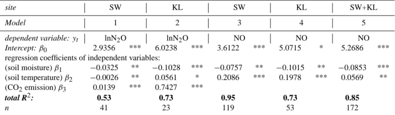
Table 6. Parameter estimation for the autoregression models 1 to 5 (Eq. 1) to predict lnN2O and NO emissions from Schottenwald and

Klausenleopoldsdorf.

site SW KL SW KL SW+KL

Model 1 2 3 4 5

dependent variable: yt lnN2O lnN2O NO NO NO

Intercept: β₀ 2.9356 *** 6.0238 *** 3.6122 *** 5.0715 * 5.2686 *** regression coefficients of independent variables:

(soil moisture) β₁ −0.0325 ** −0.1028 *** −0.0757 ** −0.1015 ** −0.0853 *** (soil temperature) β2 −0.0026 ** 0.0561 * 0.2086 *** 0.1978 *** 0.0569 **

(CO2emission) β3 0.0139 *** 0.7427 ***

total R2: 0.53 0.73 0.95 0.73 0.85

n 41 23 119 53 172

Sample period is from April 2002–May 2004 and for model 4 from August–October 2003. Regression coefficients are statistically significant at the * p<0.05, ** p<0.01, *** p<0.001 level.

Aug Dec Apr Aug Dec Apr NO [µg N m -2 h -1] -10 0 10 20 30 40 50 2002 2003 2004 (a)

Sep Oct Nov

NO [µg N m -2 h -1] 0 10 20 30 40 50 60 (b)

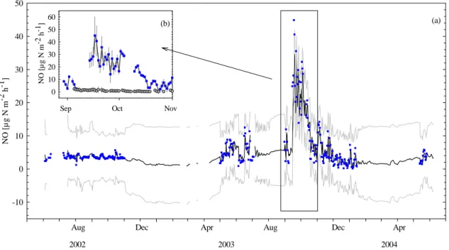
Fig. 8. (a) Measured mean (squares), predicted (black line) and confidence limits (grey line) of NO emission data in Schottenwald between

2002 and 2004. Predicted NO emissions are based on observed soil temperature and soil moisture changes (r2=0.95). Autoregressive parameters for the model (3) are shown in Table 6 (b) Comparison of emitted NO±SE in Schottenwald (squares) and Klausenleopoldsdorf (circles) between August and November 2003.

depth (x1t) and soil temperature at 5 cm soil depth (x2t),

describes daily mean NO emission with a total r2 of 0.95

(Fig. 8a). The model revealed a time-lag of 14, which means that actual NO emissions reflect changes in soil moisture and soil temperature over a period of 14 days.

At KL, NO emissions showed a significant positive corre-lation with soil (r2=0.44, p<0.001, n=66) and air tempera-ture (r2=0.66 p<0.001). There was no significant correlation

between NO and N2O emissions in KL (r2=0.29, p=0.06).

Nitric oxide emissions in KL could be predicted by soil mois-ture at a soil depth of 30 cm (x1t) and through soil tempera-ture in 5 cm soil depth (x2t) with a total r2 of 0.73 (Model 4). Expressing the prediction of NO emissions of both sites through one model (Model 5) resulted in a 5th order

autore-gressive model (lag of 5 days) with a total r2of 0.85 (Model

5). Soil moisture was the most significant (p<0.001) param-eter. Soil temperature was significant at p<0.01. Estimated parameters for the models are shown in Table 6.

3.4.4 Effects of N-input on gaseous N-emissions

To identify if N-input affects the gaseous N-emissions on longer time scales monthly mean N deposition rates were smoothed by using a moving average of 2 or 3. The

correla-tion coefficients of the mean N2O and NO monthly emission

rates measured in SW and KL and N-deposition values are outlined in Table 7. The correlation between N input and N trace gas emissions were found to be closer for KL, i.e. the less N saturated site. Correlations between N input and mean

N2O emissions were especially pronounced when calculated

from daily measurements. In KL highly significant

correla-tions between N2O emissions and deposited NO−₃ and NH+₄

via stemflow were found. In addition, a significant

corre-lation could be demonstrated for NH+₄ entering the

ecosys-tem via throughfall. In SW a significant relationship between

N2O emissions and atmospheric N-deposition could only be

demonstrated for dry deposition and NH+₄ originating from

wet (throughfall and stemflow) deposition (Table 7). Further-more, close correlations were observed between NO

emis-sions, dry NO2deposition and wet NH+4 deposition. No

cor-relation existed between NO emission and NO−₃ deposition.

Due to the short period of time regarding the measurements of NO at KL (3 months) we could not produce the same sta-tistical analysis for this site.

4 Discussion

4.1 CO2emissions

At our sites, between 70–90% of the temporal variations of soil respiration could be explained by soil temperature.

High-est CO2 emissions were detected in spring 2002, when the

increase of soil temperature and the mineralization of the

lit-ter led to a peak in CO2emissions. Zechmeister-Boltenstern

et al. (2002) found that in SW, CO2emission always peaked

in late spring due to the fast decomposition of Allium leaves, which cover the ground only from April to June.

Table 7. Correlation coefficients for significant relationships of monthly mean N-emissions and monthly N-input data at Schottenwald

and Klausenleopoldsdorf. Total N-deposition (Total Ndep) is calculated from the first investigation year (May 2002–April 2003) when dry deposition was measured.

SW KL SW KL SW lnN2O1)-manual N2O2)-AGPS NO2) TF NO−₃-N TF NH+₄-N 0.30 ** 0.32 * TF sumN 0.23 * STEM NH+₄-N 0.24 * 0.50 *** STEM NO−₃-N 0.37 ** 0.76 *** STEM N 0.36 ** 0.76 *** WET NH+₄-N 0.34 *** 0.30 * 0.46 *** 0.35 * WET NO−₃-N 0.43 *** WETsumN 0.28 ** 0.43 *** DRY NO2-N −0.50 *** −0.60 *** −0.54 ** 0.77 *** DRY NH₃-N 0.32 * 0.58 *** DRY sumN −0.48 *** −0.60 *** 0.60 ***

TF = throughfall, STEM = stemflow, WET = TF + STEM, DRY = dry deposition (1)Pearson and2)Spearman). Asterisks indicate statistic significance (* p<0.05, ** p<0.01, *** p<0.001).

Another important variable affecting respiration rates is

soil water content. Low CO2 emissions are often observed

when soils are either waterlogged or dry (Ball et al., 1999; Lee et al., 2002; Howard and Howard, 1993; Smith et al., 2003). In 2003 a continuous decrease of soil moisture was observed: from 22% at the end of May to 8% at early

September. This explains why CO2emissions measured in

the summer months of 2003 were significantly lower as com-pared to emissions measured in summer 2002. In both years and at both sites lowest emission rates were measured at the beginning of the vegetation period as a result of low tem-peratures and, subsequently, lower activity of heterotrophic microorganisms and root respiration. The overall negative

relationship between soil CO2emissions and soil water

con-tent are due to low CO2emissions in winter during periods of

high soil water content. The cumulative CO2emissions (2.3–

2.9 t C ha−1_y−1_{)from the sites (Table 4) are in good}

agree-ment with annual CO2fluxes from temperate, broad-leaved

and mixed forest soils as reported by Raich and Schlesinger (1992).

4.2 N2O emissions

During the two years of measurements N2O emissions

fol-lowed a similar seasonal trend as observed at these sites in earlier years by Meger (1997), Hahn et al. (2000) and

Zechmeister-Boltenstern et al. (2002). Highest N2O

emis-sions in SW were measured in June 2002 when soils were moist and soil temperatures were high. Schindlbacher et

al. (2004) found maximum N2O emissions at a soil

temper-ature of 20◦C and at a water-filled pore space (WFPS) of

85–95% in laboratory studies with soils from both sites. The

reported percentage of WFPS corresponds with a soil mois-ture content of 50–56% in SW and 56–63% in KL. As the soil in SW never reached the moisture optima, significantly

higher N2O emissions can be expected in the case of high

soil moisture content.

In SW the decomposition of decaying Allium leaves led to high N mineralization rates in early summer (Zechmeister-Boltenstern et al., 2002). The mineralized N was immedi-ately transformed during nitrification and denitrification re-sulting in high N2O emissions.

The meteorological conditions in the two experimental years were highly different in terms of the occurrence of dry periods and temperature maxima, thus causing pronounced interannual variations. The year 2002 was characterized by a very wet summer. In contrast meteorological conditions observed in summer 2003 showed significantly lower pre-cipitation and higher temperatures: The mean soil moisture

was about 10% lower and mean soil temperature about 0.6◦C

higher. The impact of drought in 2003 was even more pro-nounced at SW. During summer soil microbial activity, es-pecially the activity of denitrifying bacteria is strongly re-lated to water availability (Sch¨urmann et al., 2002). When soil desiccates, microbial activity is inhibited. High emis-sions were measured during the first rain after drought. In September 2003, when soil moisture increased from 9% to 12% during a precipitation event of 35 mm rainfall, a sudden

increase in N2O emissions was observed. Microorganisms

in the very dry soil produced high emissions after this rain-fall event. Comparable effects of re-wetting of dry temperate

forest soils on N2O emissions were observed by Brumme et

In the soil the concentration of NO−₃ is higher at SW as compared to the soil at KL or other soils in the region (Zechmeister-Boltenstern et al., 2002; Hackl et al., 2004); therefore nitrification might play an important role in the

pro-duction of N2O at SW. Both investigation years were

charac-terized by a dry and warm spring. As nitrification is strongly

dependent on the O2 concentration in the soil and on soil

temperature we hypothesize that, especially in spring,

nitrifi-cation was the main source of N2O production.

Generally, lowest emissions were detected in winter.

How-ever, some high winter N2O fluxes of up to 39 µg N2

O-N m−1h−1 were found after freezing and thawing events.

The winter fluxes accounted for 16%–32% of the total an-nual emissions.

The variation coefficient between the manual chambers ranged from 20% to 180% with highest variations in win-ter 2002 and in summer 2003. At both sites spatial vari-ation can be high and can be explained by different soil moisture conditions between the plots. Topographical differ-ences in the landscape alter hydrological processes and hence

N2O production/emission as previously reported by Corre et

al. (1996).

Total annual N2O emissions (mean of AGPS and manual

chambers) at SW were in the range of 0.72 and 0.79 kg N2

O-N ha−1_y−1 _{(Table 4). At the low N-input site KL annual}

N2O emissions were significantly lower (0.59 and 0.62 kg

N2O-N ha−1y−1). The calculated annual N2O emission

rates at both sites are still to some extent uncertain since e.g. in our measurements diurnal variations are not in-cluded and the location of our plots was in interstem areas which might lead to underestimations (Butterbach-Bahl et

al., 2002b). Annual N2O emissions at SW and KL were

within the same range as reported for other temperate de-ciduous forests, which have been shown to vary from 0 to

10 kg N ha−1(Brumme and Beese, 1992; Wolf and Brumme,

2003; Brumme et al., 1999; Oura et al., 2001; Papen and Butterbach-Bahl, 1999). In a Danish beech forest (N-input:

25.6 kg N ha−1y−1) N2O emissions were estimated to be

0.5 kg N ha−1_y−1_{(Beier et al., 2001).}

4.2.1 N2O emissions and N-deposition

One of the questions of our project was, whether nitrogen

deposition can have an effect on N2O emissions (Brumme et

al., 1999) at our sites. Some studies suggest that forests

re-ceiving high N-deposition are emitting higher rates of N2O

than forests exposed to low N-deposition (Castro et al., 1993; Butterbach-Bahl et al., 1997, 2002a). As a consequence of lower precipitation rates wet N-input was lower at both sites in the year 2003 as compared to the year 2002. Nitrous ox-ide emissions were found to be significantly correlated with

precipitation and N-input. In our study N2O emissions

mea-sured with high time-resolution showed a closer relationship to N-deposition than measurements with high spatial resolu-tion. At the low N-input site KL, higher and stronger

corre-lations between N2O emissions and N-deposition were

ob-served in comparison to the high N-input site SW (Table 7). These results indicate that low N-deposition sites seem to be more responsive to N-deposition events than forest sites re-ceiving chronically high rates of N deposition.

4.3 NO emissions

At SW total NO emissions in the investigation period were

0.2 and 0.5 kg N ha−1(Table 4). This considerable

interan-nual variation was mainly caused by the extremely contrast-ing weather conditions durcontrast-ing the two years. Soil moisture, followed by soil temperature, were the most important fac-tors affecting the magnitude of soil NO emissions. NO emis-sions were found to be highest at intermediate soil water con-tents (van Dijk et al., 2002). Under waterlogged conditions

NO can easily be reduced to N2O or N2before the N may

es-cape to the atmosphere (Venterea and Rolston, 2000; David-son et al., 2000). On the other hand, NO emission can also be low, when dry soil conditions constrain microbial activity (Galbally, 1989; Ludwig et al., 2001). In laboratory stud-ies (Schindlbacher et al., 2004) maximum NO emissions

oc-curred at a soil temperature of 20◦C and a WFPS of 30–45%

at SW and 65% at KL. These values correspond to a soil moisture content of 18–26% and 43% and are in good agree-ment with the environagree-mental conditions at periods with high-est NO emissions as observed by the field measurements. Rain induced pulses in NO emissions as observed at our sites in September 2003 have also been observed in seasonally dry ecosystems (Davidson, 1992; Otter et al., 1999). At SW a pulse of NO emissions, amounting to almost 50% of the an-nual emission, was recorded when soil was moistened after a long dry period, caused by a rainfall event (<35 mm). The effect of rain on dry soils may lead to a sudden burst of min-eralization and nitrification (Schmidt, 1982; Davidson et al., 1991; Williams et al., 1992). This increase of NO emissions can last several days after the water addition (Anderson and Levene, 1987; Slemr and Seiler, 1984).

At both sites (NOx-NO) was deposited. Mean daily

(NOx-NO) deposition was −2.7 µg N m−2h−1 in SW and

−0.64 µg N m−2h−1in KL. Only once we observed a weak

net emission of (NOx-NO) from the soil at the SW site

and that was in July 2003. The upward flux of (NOx-NO)

could be explained by the conversion of other nitrogen com-pounds. HONO for example might be abundant in substan-tial amounts in forest atmospheres (Kleffmann et al., 2005),

but as HONO production (from NO2) is most likely working

any time also other nitrogen compounds may contribute to

an upward flux. It has to be mentioned that NOxand O3was

measured in year 2003, but not in year 2002 where we used a filter to remove air impurities. Fluxes might have been over-estimated in the first year as the enclosed soil was exposed to

low NO concentrations. NO2which is deposited to the soil

can originate from above the canopy (by advection and sub-sequent vertical turbulent diffusion into the forest canopy)

(Jacob and Bakwin, 1992; Rummel et al., 2002; Meixner et al., 2003). On the other hand part of the NO emitted from

the soil may be converted to NO2 by reactions with ozone

that is vented into the trunkspace from the atmosphere. With

the passive diffusion tubes NO2 originating from above the

canopy but also converted NO from the soil will be captured

and has to be considered when comparing NO2 deposition

from the two systems.

4.3.1 NO emissions and N-deposition

Mean monthly NO fluxes from the soil in SW ranged

be-tween 2.1 and 21.2 µg NO-N m−2_h−1_{and were, thus}

signif-icantly (p<0.001) higher than those measured from KL. The NO emission rates at the site SW were higher than the values of a deciduous forest ecosystem (oak-hickory: 0.2–4 µg

NO-N m−2h−1)reported by Williams and Fehsenfeld (1991) and

within – or slightly lower – than reported NO emissions for

the H¨oglwald beech site in Germany (6.1–47 µg NO-N m−2

h−1)(Butterbach-Bahl et al., 1997) and for a beech forest at Sorø, Denmark (<1 kg NOxha−1y−1)(Beier et al., 2001).

At KL 0.02 kg NO-N ha−1were emitted from soil from

Au-gust to October 2003. The soil in SW received 70% more N from the atmosphere and 16 times more NO was produced (0.32 kg N ha−1). With these data we assume that there is a relationship between atmospheric N-deposition and NO flux rates at our sites.

4.4 Time series analysis

As N2O and NO emission data were autocorrelated over

time, time series analysis were conducted to predict N2O

and NO emissions from our sites taking time deferred re-lationships into account. Through the autoregression models

the temporal variation of NO and N2O emissions could be

explained by soil moisture, soil temperature as well as CO2

emission as an indicator of general microbial activity. The

results of GARCH modelling for N2O emissions of the

in-dividual sites depicted better predicted values (SW: r2=0.53

and KL: r2=0.73) compared to a simple regression model

(SW: r2=0.28 and KL: r2=0.46).

Temporal variations in NO emissions could hardly be ex-plained by a simple regression model using soil moisture and soil temperature as drivers (SW: 18% KL: 39%). However, when taking previously measured (daily mean) soil moisture and soil temperature into account up to 95% and 73% of the variations of NO emission could be explained in SW and KL, respectively. Simulation results were at their best for the year 2002, when variations between the chambers were small due to continuously high soil moisture. As a result of soil des-iccation in summer 2003 variation was higher and the fit be-tween simulated and measured values was lower.

The GARCH models revealed a 14-days deferred effect of

soil moisture and soil temperature on N2O (SW) as well as

NO (SW and KL) emissions. We could demonstrate with

this statistical procedure that at our sites emissions increased especially when soil moisture was lower (14 days before), combined with favourable soil temperature.

Modelled annual NO emissions for SW amounted to 0.18 and 0.39 kg NO-N ha−1y−1for the two years of investigation (Table 4). Using values of mean soil moisture and soil tem-perature measured daily over a period of two investigation years in order to drive the empirical model, we estimated annual NO-emissions at KL to be in the range of 0.02 and 0.03 kg NO-N ha−1y−1(Table 4).

5 Conclusions

Our results show that the temporal pattern of CO2 and

N-oxides emissions is strongly dependent on temperature. However, short-term fluctuations in N trace gas emissions can also be modulated by changes in soil moisture or freezing-thawing events. In our study significant interannual variations in the magnitude and seasonality of N trace gas emissions were demonstrated at both forest sites. Therefore, long-term measurements on a larger scale covering several years – as suggested by Ambus and Christensen (1995) – are needed to finally come up with reliable estimates of forest soil emissions.

Since we found a detectable effect of topographic

struc-tures on N2O fluxes, we hypothesize that medium scale

mea-surements in the range of several 100 m would increase the accuracy of nitrous oxide emission estimates from forests. Thus, variability caused by topographic structures could be detected.

We assume that N-input has an impact on N-emissions

at our sites. Nitric oxide emissions from the soil were

stronger affected by atmospheric N-deposition than N2O

emission. The temporal relationship between N-inputs and N-emissions was stronger for the N-limited forest ecosystem suggesting that – under increased N-input – such ecosystems can potentially function as strong sources of N trace gases in the future.

Emission data were autocorrelated over time. Therefore time series analysis was used which revealed patterns that did not become apparent through simple regression mod-els. Nitrogen oxide emissions from soils could be predicted with a higher r2. Since there are few studies in soil science which apply more complex models rather than simple regres-sion analysis, we would like to emphasize the potential of such models for data analysis and the prediction of GHG-emissions.

Acknowledgements. We would like to thank the forest managers

S. Jeitler and J. Wimmer for giving access to their properties. A. Fiege, F. Winter for field work and C. Abo-Elschabaik and M. Kitzler for helping with the sample analysis, S. Wolf for English corrections and K. Gartner for provision of meteorological data. The authors also thank K. Moder, T. Gschwantner for their

constructive work with statistics and R. Jandl and A. Schindl-bacher for comments and F. X. Meixner and three anonymous reviewers for critical discussion and editing. The study is a part of the NOFRETETE project EVK2-CT2001-00106 funded by the European Commission DG Research – Vth Framework Programme. Edited by: F. X. Meixner

References

Aber, J., McDowell, W., Nadelhoffer, K., Magill, A., Berntson, G., Kamakea, M., McNulty, S., Currie, W., Rustad L., and Fernan-dez I.: Nitrogen saturation in temperate forest ecosystems, Bio-Science, 48, 921–934, 1998.

Ambus, P. and Christensen, S.: Spatial and seasonal nitrous ox-ide and methane fluxes in Danish forest-, grassland-, and agroe-cosystems., J. Environ. Qual., 24, 993–1001, 1995.

Anderson, I. C. and Levene, J. S.: Simultaneous field measurements of nitric oxide and nitrous oxide, J. Geophys. Res., 92, 964–976, 1987.

Ball, B. C., Scott, A., and Parker, J. P.: Field N2O, CO2and CH4

fluxes in relation to tillage, compaction and soil quality in Scot-land, Soil Till. Res., 53, 29–39, 1999.

Beier, C., Rasmussen, L., Pilegaard, K., Ambus, P., Mikkelsen, T., Jensen, N. O., Kjøller, A., Priem´e, A., and Ladekarl, U. L.: Fluxes of NO−₃, NH+₄, NO, NO₂, and N₂O in an old Danish beech forest, Water, Air Soil Poll., Focus 1, 187–195, 2001. Brown, R. H.: Monitoring the ambient environment with diffusive

samplers: theory and practical considerations, J. Env. Monit., 2, 1–9, 2000.

Brumme, R. and Beese, F.: Effects of liming and nitrogen fertil-ization on emissions of CO2and N2O from temperate forest, J.

Geophys. Res., 97, 12, 851–858, 1992.

Brumme, R., Borken, W., and Finke, S.: Hierachical control on ni-trous oxide emission in forest ecosystems, Global Biogeochem. Cycl., 13, 1137–1148, 1999.

Bush, T., Smith, S., Stevenson, K., and Moorcroft, S.: Validation of nitrogen dioxide diffusion tube methodology in the UK, Atmos. Environ., 35, 289–296, 2001.

Butterbach-Bahl, K., Gasche, R., Breuer, L., and Papen, H.: Fluxes of NO and N2O from temperate forest soils: impact of forest

type, N-deposition and of liming on NO and N₂O emissions, Nutr. Cycl. Agroecosys., 48, 79–90, 1997.

Butterbach-Bahl, K., Breuer, L., Gasche, R., Willibald, G., and Pa-pen, H.: Exchange of trace gases between soils and the atmo-sphere in Scots pine forest ecosystems of the North Eastern Ger-man Lowlands, 1. Fluxes of N2O, NO/NO2and CH4at forest

sites with different N-deposition, Forest Ecol. Managem., 167, 123–134, 2002a.

Butterbach-Bahl, K., Rothe, A., and Papen, H.: Effect of tree dis-tance on N₂O and CH₄-fluxes from soils in temperate forest ecosystems, Plant Soil, 240, 91–103, 2002b.

Castro, M. S., Steudler, P. A., Melillo, J. M., Aber, J. D., and Mill-ham, S.: Exchange of N2O and CH4between the atmosphere

and soils in spruce-fir forests in the north-eastern United States, Biogeochemistry, 18, 119–135, 1993.

Corre, M. D., van Kessel, C., and Pennock, D. J.: Landscape and seasonal patterns of nitrous oxide emissions in a semiarid region, Soil Sci. Soc. Am. J., 60, 1806–1815, 1996.

Dahlgren, R. A. and Singer, M. J.: Nutrient cycling in managed and non-managed oak woodland-grass ecosystems, University of California, Davis, CA, 1994.

Davidson, E. A., Vitousek, P. M., Matson, P. A., Riley, R., Garcia-Mendez, G., and Maass, J. M.: Soil emissions of nitric oxide in a seasonally dry tropical forest of Mexico, J. Geophys. Res., 96, 15 439–15 445, 1991.

Davidson, E.: Pulses of nitric oxide and nitrous oxide flux follow-ing wettfollow-ing of dry soil: an assessment of probable sources and importance relative to annual fluxes, Ecol. Bull., 42, 149–155, 1992.

Davidson, E. A.: Soil water content and the ratio of nitrous oxide to nitric oxide emitted from soil, in: Biogeochemistry of global change, edited by: Oremland, R. S., Chapman and Hall, New York, 369–386, 1993.

Davidson, E. A. and Kingerlee, W.: A global inventory of nitric oxide emissions from soils, Nutr. Cycl. Agroecosys., 48, 37–50, 1997.

Davidson, E. A., Keller, M., Erickson, H. E., Verchot, L. V., and Veldkamp, E.: Testing a conceptual model of soil emissions of nitrous and nitric oxides, BioScience, 50, 667–680, 2000. Fitzhugh, R. D., Driscoll, C. T., Groffman, P. M., Tierney, G. L.,

Fahey, T. J., and Hardy, J. P.: Effects of soil freezing disturbance on soil solution nitrogen, phosphorus and carbon chemistry in a northern hardwood ecosystem, Biogeochemistry, 56, 215–238, 2001.

Galbally, I. E.: Factors controlling NOxemissions from soil, in:

Exchange of Trace Gases between Terrestrial Ecosystems and the Atmosphere, edited by: Andreae, M. O. and Schimel, D. S., John Wiley, New York, 23–37, 1989.

Galloway, J. N., Schlesinger, W. H., II, H. L., Michaels, A., and Schnorr, J. L.: Nitrogen fixation: anthropogenic enhancement-environmental response, Global Biogeochem. Cycl., 9, 2, 235– 252, 1995.

Gundersen, P., Emmett, B. A., and Konaas, O. J.: Impact of nitrogen deposition on nitrogen cycling in forests: a synthesis on NITREX data, Forest Ecol. Managem., 101, 37–55, 1998.

Hackl, E., Bachmann, G., and Zechmeister-Boltenstern, S.: Micro-bial nitrogen turnover in soils under different types of natural forest, Forest Ecol. Managem., 188, 101–112, 2004.

Hahn, M., Gartner, K., and Zechmeister-Boltenstern, S.: Green-house gas emissions (N₂O, CO₂ and CH₄)from beech forests near Vienna with different water and nitrogen regimes, Die Bo-denkultur – Austrian Journal of Agricultural Research, 51, 91– 101, 2000.

Hall, S. J. and Matson, P. A.: Nitrogen oxide emissions after nitro-gen additions in tropical forests, Nature, 400, 152–155, 1999. Holtermann, C.: A transportable system for the

on-line-measurement of NOx(NO, NO2)emission from soils, Die

Bo-denkultur, 47, 235–244, 1996.

Howard, D. M. and Howard, P. J.: Relationships between CO₂ evo-lution, moisture content and temperature for a range of soil types, Soil Biol. Biochem., 25, 1537–1546, 1993.

IAEA: Manual on measurements of methane and nitrous ox-ide emissions from agriculture, International Atomic Energy Agency, Vienna, 90, 1992.

Jacob, D. J. and Bakwin, P. S.: Cycling of NO in tropical forest canopies, in: Microbial Production and Consumption of Green-house Gases, edited by: Whitman, W. B., American Society of