Streamflow disaggregation: a nonlinear deterministic approach

HAL Id: hal-00302353

https://hal.archives-ouvertes.fr/hal-00302353

Submitted on 8 Sep 2004

HAL is a multi-disciplinary open access

archive for the deposit and dissemination of

sci-entific research documents, whether they are

pub-lished or not. The documents may come from

teaching and research institutions in France or

abroad, or from public or private research centers.

L’archive ouverte pluridisciplinaire HAL, est

destinée au dépôt et à la diffusion de documents

scientifiques de niveau recherche, publiés ou non,

émanant des établissements d’enseignement et de

recherche français ou étrangers, des laboratoires

publics ou privés.

approach

B. Sivakumar, W. W. Wallender, C. E. Puente, M. N. Islam

To cite this version:

B. Sivakumar, W. W. Wallender, C. E. Puente, M. N. Islam. Streamflow disaggregation: a nonlinear

deterministic approach. Nonlinear Processes in Geophysics, European Geosciences Union (EGU),

2004, 11 (3), pp.383-392. �hal-00302353�

Nonlinear Processes in Geophysics (2004) 11: 383–392

SRef-ID: 1607-7946/npg/2004-11-383

Nonlinear Processes

in Geophysics

© European Geosciences Union 2004

Streamflow disaggregation: a nonlinear deterministic approach

1_{Department of Land, Air and Water Resources, University of California, Davis, USA}

2_{Department of Biological and Agricultural Engineering, University of California, Davis, USA} 3_{Center for Computational Science and Engineering, University of California, Davis, USA} 4_{Water Resources Division, Broward County, Fort Lauderdale, Florida, USA}

∗

formerly at: Department of Land, Air and Water Resources, University of California, Davis, USA

Received: 12 May 2004 – Revised: 9 August 2004 – Accepted: 12 August 2004 – Published: 8 September 2004 Part of Special Issue “Nonlinear deterministic dynamics in hydrologic systems: present activities and future challenges”

Abstract. This study introduces a nonlinear

determinis-tic approach for streamflow disaggregation. According to this approach, the streamflow transformation process from one scale to another is treated as a nonlinear determinis-tic process, rather than a stochasdeterminis-tic process as generally as-sumed. The approach follows two important steps: (1) re-construction of the scalar (streamflow) series in a multi-dimensional phase-space for representing the transforma-tion dynamics; and (2) use of a local approximatransforma-tion (near-est neighbor) method for disaggregation. The approach is employed for streamflow disaggregation in the Mississippi River basin, USA. Data of successively doubled resolutions between daily and 16 days (i.e. daily, 2-day, 4-day, 8-day, and 16-day) are studied, and disaggregations are attempted only between successive resolutions (i.e. 2-day to daily, 4-day to 2-day, 8-day to 4-day, and 16-day to 8-day). Comparisons between the disaggregated values and the actual values re-veal excellent agreements for all the cases studied, indicating the suitability of the approach for streamflow disaggregation. A further insight into the results reveals that the best results are, in general, achieved for low embedding dimensions (2 or 3) and small number of neighbors (less than 50), suggesting possible presence of nonlinear determinism in the underlying transformation process. A decrease in accuracy with increas-ing disaggregation scale is also observed, a possible implica-tion of the existence of a scaling regime in streamflow.

1 Introduction

Streamflow disaggregation has been and continues to be a challenging problem in hydrology. The past few decades have witnessed numerous studies addressing the streamflow disaggregation problem and, consequently, a large number of mathematical models (e.g. Harms and Campbell, 1967; Va-lencia and Schaake, 1972; Salas et al., 1980; Stedinger and

Correspondence to: B. Sivakumar

(sbellie@ucdavis.edu)

Vogel, 1984; Bras and Rodriguez-Iturbe, 1985; Grygier and Stedinger, 1988; Lin, 1990; Santos and Salas, 1992; Ma-heepala and Perera, 1996). The essence of such models is to develop a staging framework (e.g. Santos and Salas, 1992), where streamflow sequences are generated at a given level of aggregation and then disaggregated into component flows.

Traditionally, streamflow disaggregation approaches have involved some variant of a linear model of the form

Xt =AZt +BVt (1)

where Xt is the vector of disaggregate variables at time t ,

Zt is the aggregate variable, Vt is a vector of independent random innovations (usually drawn from a Gaussian distri-bution), and A and B are parameter matrices. The matrix A is estimated to reproduce the correlation between aggregate and disaggregate flows, whereas the matrix B is estimated to reproduce the correlation between individual disaggregate components. The many model variants that have been made available in the literature make different assumptions on the structure and sparsity of these matrices. They also apply, prior to use of Eq. (1), a variety of normalizing transfor-mations to the data to account for the fact that (monthly) streamflow data are seldom normally distributed. Summa-bility (i.e. the requirement that disaggregate variables should add up to the aggregate quantity) has also been an issue in these models, though a few studies have effectively handled this problem in some ways (e.g. Bras and Rodriguez-Iturbe, 1985; Grygier and Stedinger, 1988).

An important aspect that has to be recognized from the above models is that they present a mathematical framework where a joint distribution of disaggregate and aggregate vari-ables is specified. However, the specified model structure is parametric. It is imposed by the form of Eq. (1) and the normalizing transformations applied to the data to represent the marginal distributions. Even though, the parametric ap-proach has been shown to be effective for streamflow disag-gregation purposes, they also possess certain important draw-backs, such as the following (Tarboton et al., 1998):

1. As Eq. (1) involves linear combinations of random vari-ables, it is compatible mainly with Gaussian distribu-tions (with only a few excepdistribu-tions). Therefore, if the marginal distribution of the streamflow variables in-volved is not Gaussian, normalizing transformations are required for each streamflow component, in which case Eq. (1) would be applied to the normalized flow vari-ables. It is often difficult to find a general normaliz-ing transformation and retain statistical properties of the streamflow process in the untransformed multi-variable space; and

2. The linear nature of Eq. (1) limits it from representing any nonlinearity in the dependence structure between variables, except through the normalizing transforma-tion used.

In view of such limitations with the parametric approach, Tarboton et al. (1998) developed a nonparametric approach for streamflow disaggregation. Such a study, in fact, fol-lowed the studies by Lall and Sharma (1996) and Sharma et al. (1997), which proposed and demonstrated the use of the nonparametric approach for streamflow simulation. The non-parametric approach eliminates the drawbacks of the para-metric approach (Tarboton et al., 1998), since: (1) the nec-essary joint probability density functions are estimated di-rectly from the historic data using kernel density estimates; (2) the procedures are data driven and relatively automatic and, therefore, nonlinear dependence can be incorporated to the extent suggested by the data; and (3) difficult subjective choices as to appropriate marginal distributions and normal-izing transformations are avoided.

With regards to disaggregation in particular, since the ba-sic purpose is to determine the proportions of the aggregate flow to allocate to each subset, the real difference between the parametric and the nonparametric approaches is the fol-lowing. The parametric approach deals with the allocation problem through a “global” prescription of the associated density function and correlation structure in a transformed data domain, whereas in the nonparametric approach this problem is approached by looking at the relative proportions of the subset variables in a “local” sense. As a result, the nonparametric approach has the ability to better capture (any) variations that may lead to heterogeneous density functions and to adaptively model complex relationships between ag-gregate and disagag-gregate flows.

The nonparametric approach, presented by Tarboton et al. (1998), is certainly a significant step forward in the con-text of streamflow disaggregation (or any other hydrologic analysis), because it not only recognizes the possible nonlin-ear behavior of the streamflow (disaggregation) phenomenon but also attempts to incorporate the nonlinear dependence of the data. In regards to the issue of nonlinearity, it is appro-priate to note that the topic of “nonlinear hydrology” has already witnessed a significant progress in the last decade or so. Among the notable advances that have been made within the area of nonlinear hydrology, the finding of the pos-sible nonlinear deterministic nature of hydrologic

phenom-ena (e.g. Rodriguez-Iturbe et al., 1989) has received arguably the widest attention (both positively and negatively). This is particularly the case in streamflow studies (e.g. Jayawardena and Lai, 1994; Porporato and Ridolfi, 1997; Krasovskaia et al., 1999; Jayawardena and Gurung, 2000; Sivakumar et al., 2001a, 2002a, b; Lisi and Villi, 2001; Islam and Sivakumar, 2002). For further details, the reader is referred to the articles by Sivakumar (2000, 2004).

The above studies have brought encouraging news for hy-drologists, in particular streamflow modelers, as they re-vealed the possible presence of nonlinear determinism in the seemingly highly irregular hydrologic phenomena, suggest-ing the possibility of accurate short-term predictions. This has further been verified and supported by the near-accurate predictions achieved for streamflow data observed at differ-ent river systems (e.g. Porporato and Ridolfi, 1997; Jayawar-dena and Gurung, 2000; Sivakumar et al., 2001a, 2002a, b; Lisi and Villi, 2001; Islam and Sivakumar, 2002) and also for other hydrologic and geomorphic data, such as lake vol-ume (e.g. Abarbanel and Lall, 1996) and suspended sediment concentration (e.g. Sivakumar, 2002).

In the spirit of such studies, an attempt is made in the present study to use the relevant ideas for streamflow dis-aggregation purposes. It is appropriate to note that such an attempt is not entirely new to hydrology, as the first author and his colleagues have previously used such ideas for rain-fall disaggregation (Sivakumar et al., 2001b). As the present study is, in a way, an extension of the study by Sivakumar et al. (2001b) as far as the field of hydrology is concerned, its originality must only be assessed from a hydrologic problem (i.e. streamflow disaggregation) point of view, rather than from a methodological perspective. Having said that, the study by Sivakumar et al. (2001b) encountered an important problem in implementing the disaggregation procedure, es-sentially due to the presence of zero rainfall values. It is the authors’ opinion that such a problem is either completely or largely overcome (depending upon the river system) when one is dealing with streamflow data, since the probability of occurrence of no flow is almost zero for large rivers and significantly low for others (compared to the probability of no rain situation). This is particularly the case for annual and monthly streamflow data, used in most of the previous streamflow disaggregation studies.

For the purpose of streamflow disaggregation in the present study, data observed in the Mississippi River basin (at St. Louis, Missouri), USA, are considered (recent re-search on the flow series from the basin has provided clues to the possible presence of nonlinear deterministic behav-ior in the underlying dynamics; Sivakumar and Jayawar-dena, 2002). Streamflow data of successively doubled res-olutions (i.e. scales) between daily and 16 days, i.e. daily, 2-day, 4-2-day, 8-2-day, and 16-2-day, are studied. Disaggregations are made only between successive resolutions, i.e. 2-day to daily, 4-day to 2-day, 8-day to 4-day, and 16-day to 8-day. The nonlinear local approximation disaggregation procedure proposed by Sivakumar et al. (2001b), with required modi-fications for streamflow data, is employed. The accuracy of

B. Sivakumar et al.: Streamflow disaggregation: a deterministic approach 385 disaggregation is measured using four different indicators:

(1) correlation coefficient; (2) root mean square error; (3) di-rect time series plots; and (4) scatter diagrams.

The organization of this paper is as follows. Section 2 presents a brief account of the nonlinear deterministic dis-aggregation procedure, originally proposed by Sivakumar et al. (2001b). Section 3 presents the details of the Mississippi River basin and the streamflow data considered in this study. Details of the disaggregation analysis carried out, results ob-tained and their discussion are reported in Sect. 4. Conclu-sions from the present study and the scope for further re-search are presented in Sect. 5.

2 Nonlinear deterministic disaggregation procedure

In a recent study, Sivakumar et al. (2001b) proposed a non-linear deterministic disaggregation approach for rainfall and also demonstrated its effectiveness on the rainfall data ob-served in the Leaf River basin in Mississippi, USA. As this approach is employed in the present study for streamflow dis-aggregation, the procedure is described below.

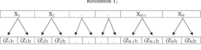
Let us assume that we have a streamflow series Xi, i=1, 2,..., N , at a certain resolution T1, and the task is to obtain

the (disaggregated) streamflow values (Zi)k, k=1, 2,..., p, at a higher (or finer) resolution T2, where p=T1/T2. Let us

also assume that the values of Xi are distributed into (Zi)k according to (Zi)k=(Wi)k*Xi, where (Wi)k are the distri-butions of weights of Xi to (Zi)k and

p

P

k=1

(Wi)k=1. As the present study considers, for the purpose of convenience, only streamflow data at successively doubled temporal reso-lutions for disaggregation purposes, the parameter p is given by p=T1/T2=2. A schematic diagram depicting such a

disag-gregation situation is presented in Fig. 1.

As the purpose is streamflow disaggregation (rather than prediction), the procedure is simplified by working with only the available streamflow series (rather than predict-ing/generating the future streamflow values and disaggregat-ing them). Let us now assume that information is available about the history of distributions of weights (Wi)k (or Xi and (Zi)k), i=1, 2,..., n, where n<N , and the task at hand is to obtain the distributions of weights (Wi)kand, hence, the streamflow values (Zi)k at a finer resolution, where i=n+1,

n+2,..., N and k=1, 2,..., p. In other words, streamflow val-ues Xi, i=1, 2,..., n, are used as the “training set” for the model to learn the dynamics of disaggregation (or transfor-mation), whereas streamflow values Xi, i=n+1, n+2,..., N are used as the testing test to assess the model performance. Based on these information, the nonlinear deterministic dis-aggregation approach is developed as follows. The procedure adopted in the model is somewhat similar to the one gener-ally used for prediction of nonlinear deterministic time series (e.g. Farmer and Sidorowich, 1987; Casdagli, 1989, 1991).

As the basic problem is to understand the dynamic changes that take place in the streamflow transformation process, it is first of all necessary to represent the evolution of the

un-Resolution T1 X1 X2 . . XN-1 XN (Z1)1 (Z1)2 (Z2)1 (Z2)2 . . . . (ZN-1)1 (ZN-1)2 (ZN)1 (ZN)2 Resolution T2 (= T1/2) Figure 1

Fig. 1. Schematic representation of distributions of weights of streamflow transformation from one resolution to another.

derlying mechanism(s). This can be done by reconstructing the multi-dimensional phase-space from the available single-dimensional series, Xi, where i=1, 2,..., N , as follows (e.g. Takens, 1981):

Yj =(Xj, Xj +τ, Xj +2τ, ..., Xj +(m−1)τ) (2)

where j =1, 2,..., N − (m − 1)τ /1t, m is the dimension of the vector Yj, called as embedding dimension, and τ is the delay time taken to be some suitable multiple of the sampling time 1t. Such a reconstruction (in a correct m dimension) allows making connection between the current state (i.e. Yj) and the future state (i.e. Yj +T) through a functional relationship

Yj +T =fT(Yj) (3)

An appropriate expression for fT (i.e. FT) is found using a local approximation technique (e.g. Farmer and Sidorowich, 1987), which entails the subdivision of the fT domain into many subsets (neighborhoods), each of which identifies some approximations FT, valid only in that subset.

With the above information, let us now consider determin-ing how the streamflow data Xn+1(i.e. the value at time n+1)

at resolution T1is disaggregated to values at resolution T2,

i.e. determining the distributions of weights (Wn+1)k. The phaspace for this case can be reconstructed using the se-ries Xi, i=1, 2,..., n+1, according to Eq. (2), where j =1, 2,..., (n+1) − (m − 1)τ /1t . Then, the disaggregation of Xn+1 is made based on Yj, j =(n+1) − (m − 1)τ /1t, and its neighbors Y0_j for all j0<j. The neighbors of Yjare found on the basis of the minimum values of ||Yj−Y0j||. If only one neighbor is considered, then the distributions of weights (Wn+1)k of Xn+1 would be the distributions of weights of

the corresponding element Xjin the nearest vector Y0_j. This is called the zeroth-order approximation. An improvement to this is the first-order approximation, which considers k0 num-ber of neighbors, and the distributions of weights (Wn+1)kof

Xn+1 is taken as an average of the k0 values’ distributions

of weights of the corresponding elements Xj in the nearest vectors. The optimal value of k0 (i.e. k_opt0 ) is determined by trial and error (e.g. Casdagli, 1991). Having determined the weights, the disaggregation of flow value Xn+1observed at

the resolution T1to flow values (Zn+1)k at resolution T2is

obtained according to (Zn+1)k=(Wn+1)k*Xn+1.

The above procedure is repeated to obtain the distributions of weights of streamflow values Xn+2, Xn+3,..., XN, i.e. (Wn+2)k, (Wn+3)k,..., (WN)k, and hence the streamflow val-ues at the resolution T2, i.e. (Zn+2)k, (Zn+3)k,..., (ZN)k. The

Table 1. Statistics of Streamflow Data of Different Temporal Resolutions in the Mississippi River Basin at St. Louis, Missouri

(Unit=m3s−1ds, where ds is the scale of observation in days).

Statistic Daily 2-day 4-day 8-day 16-day

Number of data 8192 4096 2048 1024 512 Mean 5513.9 11027.7 22055.4 44110.8 88221.6 Standard deviation 3462.6 6908.1 13713.4 26995.2 52251.5 Maximum value 24100 48100 94300 183300 338500 Minimum value 980 1990 4030 8280 17430 Coefficient of variation 0.6280 0.6264 0.6218 0.6120 0.5923 Skew 1.4779 1.4771 1.4704 1.4559 1.4122 Kurtosis 2.5031 2.5081 2.5078 2.5066 2.3898

accuracy of disaggregation can be evaluated by comparing the actual and the modeled disaggregated values using any of the standard statistical measures. In the present study, the disaggregation accuracy is evaluated using correlation coeffi-cient (CC) and root mean square error (RMSE). Time series plots and scatter diagrams are also used to choose the best disaggregation results, among a large combination of results achieved with varying number of neighbors and embedding dimensions.

3 Study area and data used

In the present study, river flow data observed in the Missis-sippi River basin is studied to evaluate the performance of the nonlinear deterministic disaggregation approach. The Mis-sissippi River, because of its enormous size and quantity of flow, plays a major role in fulfilling various water demands in a number of states in the United States and also in parts of Canada. However, the river’s size and quantity of flow are also primary reasons for the flooding and sediment transport problems faced in these regions. The frequent floods in the Mississippi River cause extensive losses of life and property. The river is also a dominant mover of sediment and trans-ports more sediment than any other river in North America (e.g. Meade and Parker, 1985), in spite of the large dams that have been built across its major tributaries. Discharging as large as about 230 million tons of suspended sediment per year to the coastal zone, the Mississippi River ranks sixth in the world in suspended sediment transport to the oceans (e.g. Milliman and Meade, 1983). The extensive flooding and sediment transport problems caused by the Mississippi River, often within the order of a few days, necessitate ac-curate flow data at much higher resolutions than that are cur-rently available, in order for flood forecasting and emergency measures to be effective. For this reason, in the present study, flow data observed in the Mississippi River basin is studied for streamflow disaggregation purposes, in order to evaluate the performance of the nonlinear deterministic disaggrega-tion approach.

Flow data in the Mississippi River basin are measured at a large number of locations throughout the basin. For the

present study, flow data observed in a sub-basin station of the Mississippi River basin at St. Louis in the State of Missouri (US Geological Survey station no. 07010000) are considered. The sub-basin is situated at 38◦3700300latitude and 90◦1004700 longitude, on downstream side of west pier of Eads Bridge at St. Louis, 24.1 km downstream from Missouri River. The drainage area of this sub-basin is 251 230 km2 (e.g. Chin et al., 1975). The natural flow of stream at this gaging station is affected by many reservoirs and navigation dams in the upper Mississippi River basin and by many reservoirs and diversions for irrigation in the Missouri River basin.

For the above station, daily flow measurements have been made available from April 1948. However, there were some missing data before 1960. As the use of continuous data eliminates the possible uncertainties on data quality (that could arise from interpolation and other schemes if the record were to contain missing data), it is decided to use only the data measured starting from 1 January 1961. The data con-sidered in this study are those measured over a period of about 22.5 years from 1961 to 1983 (amounting to 8192 val-ues).

To evaluate the effectiveness of the disaggregation ap-proach, an aggregation-disaggregation scheme (aggregation followed by disaggregation) is used. First, the above daily flow values are aggregated (by simple addition) to obtain flow data at four successively doubled lower resolutions (i.e. 2-day, 4-day, 8-day, and 16-day). The nonlinear determin-istic disaggregation approach is then employed to disaggre-gate these aggredisaggre-gated data series to obtain flow data at the successively doubled finer resolutions (i.e. from 16-day to 8-day, from 8-day to 4-day, from 4-day to day, and from 2-day to daily). Table 1 presents some of the important statis-tics of these five flow series. As the minimum values indi-cate, there are no zero values in the flow series. This elimi-nates the problems faced by Sivakumar et al. (2001b) in their study of disaggregation of rainfall series observed in the Leaf River basin, even though this cannot be generalized for every streamflow series.

Each of the above five series is used as follows in the im-plementation of the disaggregation procedure. The entire se-ries is divided into two halves. The first half of the sese-ries

B. Sivakumar et al.: Streamflow disaggregation: a deterministic approach 387

Table 2. 2-day to Daily Streamflow Disaggregation Results in the Mississippi River Basin at St. Louis, Missouri.

Embedding Correlation Root mean square Optimal number of

dimension (m) coefficient (CC) error (RMSE) neighbors (k_opt0 )

1 0.9981 260.867 150 2 0.9990 187.025 10 3 0.9991 183.801 3 4 0.9989 196.865 5 5 0.9988 207.081 10 6 0.9987 216.099 10 7 0.9986 227.645 5 8 0.9985 230.183 5 9 0.9985 234.772 10 10 0.9984 238.474 10

is used for phase-space reconstruction to represent the dy-namics of the disaggregation process. As the phase-space reconstruction is, in a way, done as a “training” or “learn-ing” procedure to understand how the coarser (i.e. lower) resolution series is disaggregated into the next finer resolu-tion series, such a set is called “training set” or “learning set.” Based on such a training procedure, the disaggrega-tion is made only for one-fourth of the second half of the series (that immediately follows the first half). This latter set, essentially used to verify the effectiveness of the dis-aggregation procedure through comparison between actual and modeled disaggregated values, is called the “testing set.” Therefore, the training and testing sets are selected in such a way that disaggregation is made for the same period, ir-respective of the disaggregation resolution. This is done, as it would allow useful and consistent comparisons between the disaggregation results obtained for the four disaggrega-tion cases. This, in turn, could provide important informadisaggrega-tion about the performance or effectiveness of the nonlinear de-terministic disaggregation scheme with respect to changing (increasing/decreasing) scales.

4 Analysis, results and discussion

4.1 Analysis and results

The nonlinear deterministic disaggregation approach is now employed to the above flow series. As mentioned above, dis-aggregation between only successively doubled resolutions (i.e. p=2) is considered. For each of the four disaggrega-tion cases, the flow series is reconstructed in phase-spaces or embedding dimensions (m) from 1 to 10 to represent the transformation dynamics, and the number of neighbors (k0) used in the disaggregation procedure is varied from 1 to 200. However, to reduce the computational time, only nine differ-ent combinations of numbers of neighbors (i.e. 1, 2, 5, 10, 20, 50, 100, 150, and 200) are considered. These combinations

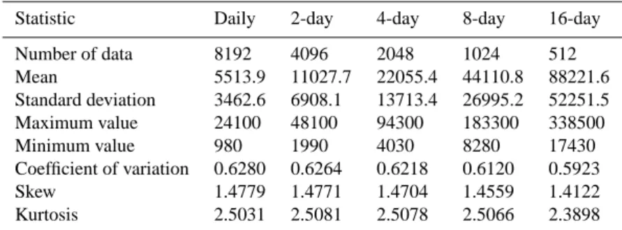
Figure 2(a) Figure 2(b) 0.996 0.997 0.998 0.999 1.000 1 10 100 1000 Number of Neighbors C or re la tio n C oe ff ic ie nt m = 1 m = 2 m = 3 m = 4 m = 5 m = 6 m = 7 m = 8 m = 9 m = 10 100 150 200 250 300 350 400 450 1 10 100 1000 Number of Neighbors R oo t M ea n Sq ua re E rr or m = 1 m = 2 m = 3 m = 4 m = 5 m = 6 m = 7 m = 8 m = 9 m = 10 (a) Figure 2(a) Figure 2(b) 0.996 0.997 0.998 0.999 1.000 1 10 100 1000 Number of Neighbors C or re la tio n C oe ff ic ie nt m = 1 m = 2 m = 3 m = 4 m = 5 m = 6 m = 7 m = 8 m = 9 m = 10 100 150 200 250 300 350 400 450 1 10 100 1000 Number of Neighbors R oo t M ea n Sq ua re E rr or m = 1 m = 2 m = 3 m = 4 m = 5 m = 6 m = 7 m = 8 m = 9 m = 10 (b) Fig. 2. Effect of number of neighbors on the performance of disag-gregation of 2-day streamflow to daily streamflow in the Mississippi River basin at St. Louis, Missouri: (a) correlation coefficient; and (b) root mean square error.

are chosen (at different, but appropriate, intervals) in such a way that the results would be able to reflect the sensitivity of the disaggregation results to the number of neighbors used in the disaggregation procedure.

With the above general information, the streamflow dis-aggregation results obtained for each of the four disaggre-gation cases using the nonlinear deterministic procedure are presented in this section. However, for the purpose of brevity, detailed results are presented only for the case of disaggrega-tion of flow from 2-day to daily, and for the remaining three cases, only the important results are highlighted.

4.1.1 Disaggregation of flow from 2-day to daily

Figures 2a and b present the accuracy of disaggregation (in terms of correlation coefficient (CC) and root mean square error (RMSE)) against the number of neighbors (for each of the ten embedding dimensions) when the 2-day flow series is disaggregated into daily flow series. As can be seen, in gen-eral, for any embedding dimension, the disaggregation accu-racy increases with increasing number of neighbors up to a certain point and then saturates (or even decreases) beyond that point. The minimum number of neighbors that corre-sponds to the above saturation point is called as the “optimal number of neighbors”, k0_opt. These results are presented in a different form in Table 2, which includes also the optimal number of neighbors. As can be seen, different k0_opt values

Table 3. 4-day to 2-day Streamflow Disaggregation Results in the Mississippi River Basin at St. Louis, Missouri.

Embedding Correlation Root mean square Optimal number of

dimension (m) coefficient (CC) error (RMSE) neighbors (k_opt0 )

1 0.9941 920.248 200 2 0.9961 745.735 20 3 0.9966 702.532 5 4 0.9958 770.948 5 5 0.9951 833.635 10 6 0.9948 860.788 10 7 0.9947 871.089 20 8 0.9945 882.668 20 9 0.9945 885.667 20 10 0.9945 882.886 20

are obtained for different embedding dimensions. Again, the disaggregation results show a trend of increase in accuracy with increasing embedding dimension up to a certain point and then saturation (or even decrease) in accuracy beyond that point. The smallest embedding dimension correspond-ing to such a saturation point is called as the “optimal em-bedding dimension”, mopt.

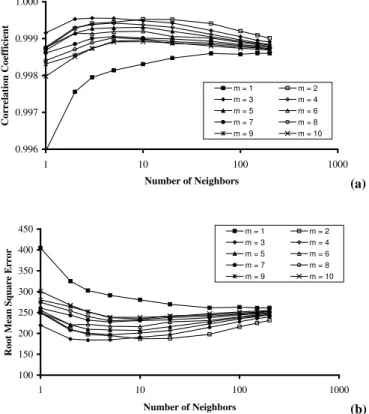
Figure 2 and Table 2 indicate that, even though almost all of the ten combinations of m and nine combinations of k0 yield very good results, the best disaggregation results (with CC=0.9991, RMSE=183.801) are achieved when the embedding dimension is 3 and the number of neighbors is 3, i.e. mopt=3 and kopt0 =3 (indicated in bold in Table 2). For this case, Fig. 3 presents comparisons, using scatter diagram (with the solid 1:1 diagonal line shown for reference), of the actual daily flow series and the daily flow series disag-gregated from the 2-day series (time series and scatter di-agram comparisons for different combinations of m and k0 (figures not shown) also indicate that the best results are in-deed achieved for m=3 and k0=3). As can be seen, the dis-aggregated flow values are in excellent agreement with the actual flow values, as the points are lying on an almost per-fect diagonal line.

The fact that the best disaggregation results are achieved for m=3 could be an indication that a three-dimensional phase-space is essential to represent the important dynam-ics involved in the flow transformation process between 2-day and daily scales. In other words, the transformation dy-namics may be governed by only three dominant variables or mechanisms. This seems to suggest that the disaggre-gation dynamics can be understood and modeled through a low-dimensional approach. The near-accurate disaggrega-tion results achieved using such an approach seem to pro-vide further support to the above. The observations of low mopt (=3) and small kopt0 (=3) values also seem to present clues to the presence of low-dimensional deterministic be-havior in the underlying transformation dynamics (e.g. Cas-dagli, 1989, 1991). Figure 3 0 5000 10000 15000 20000 25000 0 5000 10000 15000 20000 25000 Observed Streamflow (m3_s-1_d s) M od el ed S tr ea m flo w (m 3s -1d s )

Fig. 3. Comparison between modeled and observed disaggregated values of 2-day streamflow to daily streamflow in the Mississippi River basin at St. Louis, Missouri. The results are for embedding

dimension (m)=3 and number of neighbors (k0)=3.

At this stage, it is relevant to discuss the decrease in dis-aggregation accuracy beyond mopt and kopt0 . If the under-lying transformation dynamics is low-dimensional determin-istic, then, conceptually, the disaggregation accuracy should increase with increase in embedding dimension up to a cer-tain point (i.e. mopt)and attain saturation beyond that point. A similar conceptual definition also applies for the number of neighbors, where saturation in disaggregation accuracy should be attained beyond k_opt0 . However, the results ob-tained for the case of flow disaggregation from 2-day to daily, presented in Table 2 and Fig. 2, reveal a slightly different story. While, as expected, an increase in disaggregation accu-racy up to mopt (Table 2) and k0opt(Fig. 2) is observed, there is no saturation in disaggregation accuracy beyond mopt and

k0_opt, but a decrease in accuracy is observed. This is surpris-ing considersurpris-ing the fact that any dimension beyond mopt (for a particular k0_{) or any number of neighbors beyond k}0

opt (for a particular m) potentially include only additional informa-tion about the dynamics in the phase-space reconstrucinforma-tion or in the disaggregation procedure, as the case may be.

Having said that, the above pure theoretical explanation and expectation is valid only for noise-free data series, such as artificially generated ones. As noise is a prominent lim-iting factor in the phase-space reconstruction and neighbor searching procedures (e.g. Schreiber and Kantz, 1996), such a theoretical expectation is difficult to meet with when one deals with real data, which are always contaminated with noise. The effect of noise (on prediction/disaggregation) with respect to embedding dimension and number of neigh-bors are discussed in detail in Sivakumar et al. (1999, 2001a, b, 2002a, b) and, therefore, are not reported herein.

4.1.2 Disaggregation of flow from 4-day to 2-day, 8-day to 4-day, and 16-day to 8-day

Tables 3, 4, and 5 summarize the results of disaggregation of flow from 4-day to 2-day, from 8-day to 4-day, and from 16-day to 8-day, respectively. The results presented therein, for each case, are the best results achieved for each of the

B. Sivakumar et al.: Streamflow disaggregation: a deterministic approach 389

Table 4. 8-day to 4-day Streamflow Disaggregation Results in the Mississippi River Basin at St. Louis, Missouri.

Embedding Correlation Root mean square Optimal number of

dimension (m) coefficient (CC) error (RMSE) neighbors (k_opt0 )

1 0.9892 2470.02 200 2 0.9902 2350.76 50 3 0.9899 2381.36 50 4 0.9898 2401.80 100 5 0.9897 2411.06 100 6 0.9896 2425.62 100 7 0.9896 2418.28 150 8 0.9896 2425.59 200 9 0.9894 2440.80 200 10 0.9894 2445.44 200

ten embedding dimensions used in the phase-space recon-struction, with the optimal number of neighbors for each di-mension is also presented. From these results, the following general observations may be made:

1. The disaggregation accuracy is very high for all of the three disaggregation cases (with CC>0.974), irrespec-tive of the embedding dimension used for the phase-space reconstruction;

2. The best disaggregation results are near-accurate (with CC>0.975);

3. The best disaggregation results are achieved when the embedding dimension is low, i.e. typically 2 or 3 (the only exception to this is the case of disaggregation from 16-day to 8-day, where m=8 yields the best results, and m=10 and m=3 yield, in order, the next best results) (in-dicated in bold in Tables 4, 5, and 6);

4. The best disaggregation results are achieved when the number of neighbors is small, i.e. typically below 20 (an exception to this is the case of disaggregation from 8-day to 4-day, for which k0=50 yields the best results); and

5. The disaggregation accuracy decreases with increasing scale of aggregation, with the best results for the case of disaggregation from 4-day to 2-day and the worst for the case of disaggregation from 16-day to 8-day. The first four of these observations are consistent with the observations made earlier for the case of disaggregation from 2-day to daily. Also, a comparison of the results for all of the above four disaggregation cases supports the fifth observa-tion, with the best results obtained for the case of disaggre-gation from 2-day to daily (see below more further details).

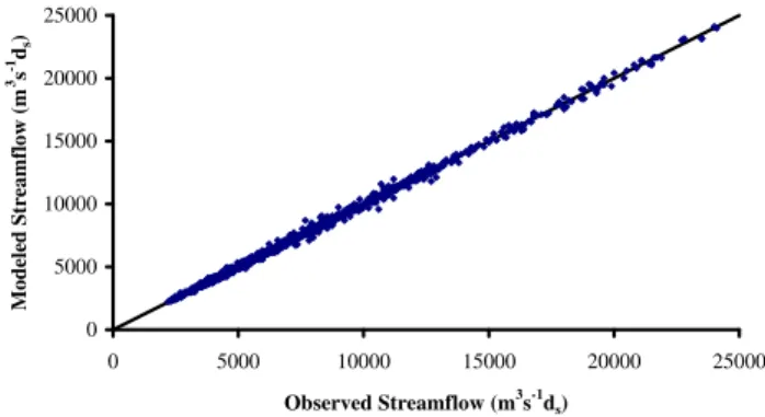
Figures 4, 5, and 6 compare, through scatter diagrams, the actual and modeled disaggregated values for the cases of dis-aggregation from 4-day to 2-day, from 8-day to 4-day, and

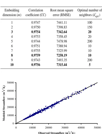
Table 5. 16-day to 8-day Streamflow Disaggregation Results in the Mississippi River Basin at St. Louis, Missouri.

Embedding Correlation Root mean square Optimal number of

dimension (m) coefficient (CC) error (RMSE) neighbors (k0_opt)

1 0.9747 7441.11 100 2 0.9750 7398.83 150 3 0.9754 7342.64 20 4 0.9753 7358.45 20 5 0.9744 7478.98 200 6 0.9751 7388.94 10 7 0.9755 7325.99 10 8 0.9759 7258.19 10 9 0.9743 7493.35 200 10 0.9756 7315.44 5 Figure 4 0 10000 20000 30000 40000 50000 0 10000 20000 30000 40000 50000 Observed Streamflow (m3_s-1_d s) M od el ed S tr ea m flo w (m 3s -1d s )

Fig. 4. Comparison between modeled and observed disaggregated values of 4-day streamflow to 2-day streamflow in the Mississippi River basin at St. Louis, Missouri. The results are for embedding

dimension (m)=3 and number of neighbors (k0)=5.

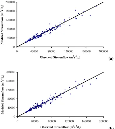
from 16-day to 8-day, respectively. The results shown are the best results achieved for each of these three cases (except for the last case), and are chosen from Tables 3, 4, and 5, respec-tively. In the case of disaggregation from 16-day to 8-day, re-sults corresponding to two different combinations: (1) m=3 and k0=20 (Fig. 6a); and (2) m=8 and k0=10 (Fig. 6b), are shown. This is done because these two combinations yield almost similar results but represent phase-space reconstruc-tions at low and high embedding dimensions, respectively, and, therefore, might provide interesting observations and fa-cilitate better comparisons and interpretations.

As can be seen from Figs. 4, 5, and 6, there are, in general, excellent agreements between the actual and modeled disag-gregated flow values for each of the three cases (as for Fig. 6, while an unambiguous identification of the better combina-tion is not easy, the combinacombina-tion of m=8 and k0=10 seems to have an edge over that of m=3 and k0=20). This indicates the suitability of the nonlinear deterministic approach for under-standing and modeling the flow disaggregation dynamics at these disaggregation scales. Also, a decrease in disaggrega-tion accuracy with increasing scale of aggregadisaggrega-tion is clearly evident from the scatter diagrams.

Figure 5 0 20000 40000 60000 80000 100000 0 20000 40000 60000 80000 100000 Observed Streamflow (m3_s-1_d s) M od el ed S tr ea m flo w (m 3s -1d s )

Fig. 5. Comparison between modeled and observed disaggregated values of 8-day streamflow to 4-day streamflow in the Mississippi River basin at St. Louis, Missouri. The results are for embedding

dimension (m)=2 and number of neighbors (k0)=50.

Figure 6(a) Figure 6(b) 0 40000 80000 120000 160000 200000 0 40000 80000 120000 160000 200000 Observed Streamflow (m3_s-1_d s) M od el ed S tr ea m flo w (m 3s -1d s ) 0 40000 80000 120000 160000 200000 0 40000 80000 120000 160000 200000 Observed Streamflow (m3_s-1_d s) M od el ed S tr ea m flo w (m 3s -1d s ) (a) Figure 6(a) Figure 6(b) 0 40000 80000 120000 160000 200000 0 40000 80000 120000 160000 200000 Observed Streamflow (m3_s-1_d s) M od el ed S tr ea m flo w (m 3s -1d s ) 0 40000 80000 120000 160000 200000 0 40000 80000 120000 160000 200000 Observed Streamflow (m3_s-1_d s) M od el ed S tr ea m flo w (m 3s -1d s ) (b) Fig. 6. Comparison between modeled and observed disaggregated values of 16-day streamflow to 8-day streamflow in the Mississippi River basin at St. Louis, Missouri: (a) embedding dimension (m)=3

and number of neighbors (k0)=20; and (b) embedding dimension

(m)=8 and number of neighbors (k0)=10.

4.2 Discussion of results

The decrease in disaggregation accuracy with increasing scale of aggregation may seem contradictory, since it is gen-erally (but not necessarily) believed that data at coarser res-olutions are less irregular when compared to that at finer resolutions and, thus, are easier to deal with. Even if this belief/expectation exists, it should be noted, in the present case, that the transformation process between any two scales

is entirely different from the evolution process at the two in-dividual scales. Therefore, when the task at hand is disag-gregation, “coarser resolutions” do not necessarily mean less irregular than “finer resolutions.” In view of this, the present results could indeed be an actual reflection of the reality of the flow transformation process at the four disaggregation resolutions considered. On the other hand, the above results could also be an indication of the “scaling range” present in the river flow process. That is, a clear scaling range may ex-ist between daily and 8-day scales (where the disaggregation procedure is much more effective), and may disappear grad-ually beyond such a resolution. Whether or not this is indeed true needs to be investigated by studying resolutions coarser than 16 days.

Having said that, it is also possible that the aggregation procedure used to obtain data sets at different (coarser) reso-lutions could hamper the ability of the present disaggregation procedure in providing accurate results. This is essentially because the coarser resolution data series (e.g. 16-day) con-tain, in all probability, higher levels of noise than the finer resolution series (e.g. daily), considering the facts that the finest resolution series (i.e. daily) itself is contaminated with noise and that data at other resolutions are obtained by sim-ply adding the appropriate (number of) daily values. The presence of noise in the data series of two different resolu-tions certainly brings noise to the transformation (i.e. distri-butions of weights) between the two resolutions. As a result, the distributions of weights at coarser resolutions would, in all probability, contain higher level of noise than that at finer resolutions. The issue of noise on the outcomes of the disag-gregation procedure has already been discussed and, there-fore, is not reiterated at this stage.

One other observation that is worthy of mention is con-cerned with the pattern of behavior (or lack thereof) in the disaggregation accuracy with respect to the embedding di-mension and the number of neighbors, for the four flow dis-aggregation cases studied. For the case of disdis-aggregation from 2-day to daily (Table 2 and Fig. 3), there is a definite pattern of increase in disaggregation accuracy with an in-crease in m and k0 and then a decrease with further increase in m and k0 (except for m=1, in which case the phase-space is largely inadequate). There is also some consistency in the k0_opt for each m (k_opt0 typically below 10). These patterns are observed also for the cases of disaggregation from 4-day to 2-day (with k_opt0 typically below 50) (Table 3) and from 8-day to 4-day (with k0

opt typically above 100, except for m=2 and

m=3) (Table 4). In other words, clear mopt and kopt0 exist for these three cases. However, no definite pattern is observed for the case of disaggregation from 16-day to 8-day (Table 5), where the disaggregation accuracy fluctuates, in an irregular manner, with respect to both m and k0. The k_opt0 for each malso fluctuates significantly, ranging from 5 to 200. What causes this situation is not clear at this moment, and further investigations are needed in this area.

B. Sivakumar et al.: Streamflow disaggregation: a deterministic approach 391 However, the fluctuation with respect to m seems to start

at m=4, and there still seems to be a trend of increase in disaggregation accuracy up to m=3, suggesting that a three-dimensional phase-space could still be sufficient for this case, just as it is for the other cases (for which mopt is typi-cally 2 or 3). The fact that there is no significant difference between the results obtained at m=3 and at m=8 only seems to support the above. However, one has to be cautious in pro-viding such interpretations and conclusions, since there is al-ways a possibility of getting trapped into a “local optimum” rather than finding a “global optimum”. The determination of mopt and k0opt in the present disaggregation procedure (or any phase-space reconstruction and neighbor searching pro-cedure for that matter) is in itself an important problem to be addressed, details of which are not discussed herein (the interested reader is referred to, for instance, Jayawardena et al. (2002) and Phoon et al. (2002) for details).

5 Summary, conclusions and future research potential

The present study introduced a nonlinear deterministic ap-proach for streamflow disaggregation that treats the dy-namics of flow transformation between (two) scales as a deterministic chaotic process. As per this approach, the flow transformation dynamics was represented first using a phase-space reconstruction procedure and then disaggrega-tion was made using a local approximadisaggrega-tion (nearest neigh-bor) method. The performance of the approach was tested on the streamflow series observed in the Mississippi River basin (at St. Louis, Missouri), USA. Specifically, flow series of successively doubled resolutions between daily and 16 days (i.e. daily, 2-day, 4-day, 8-day, and 16-day) were studied, and disaggregations were made only between successive resolu-tions (i.e. 2-day to daily, 4-day to 2-day, 8-day to 4-day, and 16-day to 8-day). The results revealed the appropriateness of the nonlinear deterministic approach for streamflow dis-aggregation, as there were excellent agreements between the actual values and the modeled values for all of the four disag-gregation cases studied. In general, phase-space reconstruc-tion in lower dimensions (typically 2 or 3) yielded the best disaggregation results, a possible implication that the under-lying transformation dynamics could be dominated by only a few variables or mechanisms. The results also indicated a decrease in accuracy with a change of disaggregation scale from finer to coarser. While this could imply the existence of a particular “scaling range,” (probably between daily and 8 days in this case) where the disaggregation procedure is expected to be effective, further verification is necessary in light of the potential limitations of the present approach for noisy time series, among others.

The present study was different from the previous stream-flow disaggregation studies in two important aspects: (1) The study treated the dynamics of streamflow transformation as a nonlinear deterministic process, whereas the previous stud-ies assumed the underlying process as stochastic (through parametric or non-parametric procedures); and (2) Whereas

most, if not all, of the past studies focused on streamflow disaggregation between very coarse resolutions (e.g. annual and monthly scales), the present study attempted disaggre-gation between relatively much finer resolutions (e.g. daily and weekly scales). In regards to (1), even though a direct comparison between the present study and the past studies could not be made, due essentially to the different disaggre-gation scales studied, the near-accurate results achieved in the present study indicate the suitability of the nonlinear de-terministic approach for streamflow disaggregation. A com-parison of the performance of stochastic and nonlinear de-terministic approaches is expected to shed some light on the usefulness and appropriateness of these approaches for the specific disaggregation scale (finer or coarser) at hand, and on the selection of the better approach for that scale. Efforts are being made in this direction, details of which will be re-ported elsewhere.

It is the authors’ opinion that the present study has equal practical relevance and significance when compared to the previous studies because of the finer disaggregation scales studied, as mentioned in (2). Obtaining streamflow data at much finer resolutions (e.g. daily scales and even finer) is as equally important as that at coarser resolutions (e.g. monthly). This is because (the availability of) finer reso-lution data plays an important role in effectively forecast-ing flood events and efficiently improvforecast-ing and implement-ing flood warnimplement-ing and emergency measures, which normally (must) happen within a few days or even a few hours.

A final remark on the possibility of dealing with stream-flow disaggregation problem over all (or at least a large range of) scales is in order. As the stochastic streamflow disaggre-gation schemes have been found to provide very good results for coarser resolutions (e.g. Lin, 1990; Maheepala and Per-era, 1996; Tarboton et al., 1998) and as the present deter-ministic disaggregation procedure has been found to perform extremely well for finer resolutions, coupling of these two approaches could potentially yield better results than those that can be achieved when the two are performed indepen-dently. In this regard, the coupling of nonlinear deterministic approach and nonparametric approach (e.g. Tarboton et al., 1998) could be a first step. As these two approaches pos-sess important commonalities, such as: (1) they use historic data in the analysis (to reconstruct the phase-space or to es-timate the necessary joint probability density functions); (2) they are data driven; (3) they restore summability; (4) they view the allocation problem from a “local” sense rather than a “global” sense; and (5) they are able to incorporate the non-linear dependency that is present in the underlying dynamics, it is hoped that their coupling could be done without much difficulty. Whether this is indeed the case remains to be seen.

Acknowledgements. The authors thank the two anonymous review-ers for their constructive comments and useful suggestions on an earlier version of this manuscript.

Edited by: R. Berndtsson Reviewed by: two referees

References

Abarbanel, H. D. I. and Lall, U.: Nonlinear dynamics of the Great Salt Lake: system identification and prediction, Climate Dyn., 12, 287–297, 1996.

Bras, R. L. and Rodriguez-Iturbe, I.: Random Functions and Hy-drology, Addison-Wesley, Massachusetts, 1985.

Casdagli, M.: Nonlinear prediction of chaotic time series, Physica D, 35, 335–356, 1989.

Casdagli, M.: Chaos and deterministic versus stochastic non-linear modeling, J. Royal Stat. Soc. B, 54(2), 303–328, 1991.

Chin, E. H., Skelton, J., and Guy, H. P.: The 1973 Mississippi River Basin flood: compilation and analysis of meteorologic, stream-flow, and sediment data, US Geol. Surv. Prof. Pap., 937, 1–137, 1975.

Farmer, D. J. and Sidorowich, J. J.: Predicting chaotic time series, Phys. Rev. Lett., 59, 845–848, 1987.

Grygier, J. C. and Stedinger, J. R.: Condensed disaggregation pro-cedures and conservation corrections for stochastic hydrology, Water Resour. Res., 24(10), 1574–1584, 1988.

Harms, A. A. and Campbell, T. H.: An extension to the Thomas-Fiering model for the sequential generation of streamflow, Water Resour. Res., 3(3), 653–661, 1967.

Islam, M. N. and Sivakumar, B.: Characterization and prediction of runoff dynamics: A nonlinear dynamical view, Adv. Water Resour., 25(2), 179–190, 2002.

Jayawardena, A. W. and Gurung, A. B.: Noise reduction and predic-tion of hydrometeorological time series: Dynamical systems ap-proach vs. stochastic apap-proach, J. Hydrol., 228, 242–264, 2000. Jayawardena, A. W. and Lai, F.: Analysis and prediction of chaos

in rainfall and stream flow time series, J. Hydrol., 153, 23–52, 1994.

Jayawardena, A. W., Li, W. K., and Xu, P.: Neighborhood selection for local modeling and prediction of hydrological time series, J. Hydrol., 258, 40–57, 2002.

Krasovskaia, I., Gottschalk, L., and Kundzewicz, Z. W.: Dimen-sionality of Scandinavian river flow regimes, Hydrol. Sci. J., 44(5), 705–723, 1999.

Lall, U. and Sharma, A.: A nearest neighbor bootstrap for time series resampling, Water Resour. Res., 32(3), 679–693, 1996. Lin, G. F.: Parameter estimation for seasonal to subseasonal

disag-gregation, J. Hydrol., 120, 65–77, 1990.

Lisi, F. and Villi, V.: Chaotic forecasting of discharge time series: A case study, J. Am. Water Resour. Assoc., 37(2), 271–279, 2001. Maheepala, S. and Perera, B. J. C.: Monthly hydrologic data

gener-ation by disaggreggener-ation, J. Hydrol., 178, 277–291, 1996. Meade, R. H. and Parker, R. S.: Sediment in rivers of the United

States. National Water Summary 1984 – Hydrologic Events, Se-lected Water Quality Trends, and Groundwater Resources, US Geol. Surv. Water Supply Pap., 2275, 1–467, 1985.

Milliman, J. D. and Meade, R. H.: Worldwide delivery of river sed-iments to the oceans, J. Geol., 91, 1–9, 1983.

Phoon, K. K., Islam, M. N., Liaw, C. Y., and Liong, S. Y.: A practi-cal inverse approach for forecasting of nonlinear time series anal-ysis, J. Hydrol. Engg. ASCE, 7(2), 116–128, 2002.

Porporato, A. and Ridolfi, L.: Nonlinear analysis of river flow time sequences, Water Resour. Res. 33(6), 1353–1367, 1997.

Rodriguez-Iturbe, I., De Power, F. B., Sharifi, M. B., and Geor-gakakos, K. P.: Chaos in rainfall, Water Resour. Res., 25(7), 1667–1675, 1989.

Salas, J. D., Delleur, J. W., Yevjevich, V., and Lane, W. L.: Applied Modeling of Hydrologic Time Series, Water Resources, Little-ton, Colorado, 1980.

Santos, E. G. and Salas, J. D.: Stepwise disaggregation scheme for synthetic hydrology, J. Hyd. Engg ASCE, 118(5), 765–784, 1992.

Schreiber, T. and Kantz, H.: Observing and predicting chaotic sig-nals: Is 2% noise too much? in: Predictability of Complex Dy-namical Systems, edited by Kravtsov, Yu. A and Kadtke, J. B., Springer Series in Synergetics, Springer, Berlin, 43–65, 1996. Sharma, A., Tarboton, D. G., and Lall, U.: Streamflow simulation:

A nonparametric approach, Water Resour. Res., 33(2), 291–308, 1997.

Sivakumar, B.: Chaos theory in hydrology: important issues and interpretations, J. Hydrol., 227(1-4), 1–20, 2000.

Sivakumar, B.: Chaos theory in geophysics: past, present and fu-ture, Chaos Sol. Fract., 19(2), 441–462, 2004.

Sivakumar, B.: A phase-space reconstruction approach to predic-tion of suspended sediment concentrapredic-tion in rivers, J. Hydrol., 258, 149–162, 2002.

Sivakumar, B. and Jayawardena, A. W.: An investigation of the presence of low-dimensional chaotic behavior in the sediment transport phenomenon, Hydrol. Sci. J., 47(3), 405–416, 2002. Sivakumar, B., Phoon, K. K., Liong, S. Y., and Liaw, C. Y.: A

systematic approach to noise reduction in chaotic hydrological time series, J. Hydrol., 219, 103–135, 1999.

Sivakumar, B., Berndtsson, R., and Persson, M.: Monthly runoff prediction using phase-space reconstruction, Hydrol. Sci. J., 46(3), 377–387, 2001a.

Sivakumar, B., Sorooshian, S., Gupta, H. V., and Gao, X.: A chaotic approach to rainfall disaggregation, Water Resour. Res., 37(1), 61–72, 2001b.

Sivakumar, B., Persson, M., Berndtsson, R., and Uvo, C. B.: Is cor-relation dimension a reliable indicator of low-dimensional chaos in short hydrological time series? Water Resour. Res., 38(2), 10.1029/2001WR000333, 2002a.

Sivakumar, B., Jayawardena, A. W., and Fernando, T. M. G. H.: River flow forecasting: Use of phase-space reconstruction and artificial neural networks approaches, J. Hydrol., 265(1-4), 225– 245, 2002b.

Stedinger, J. R. and Vogel, R. M.: Disaggregation procedures for generating serially correlated flow vectors, Water Resour. Res., 20(11), 47–56, 1984.

Takens, F.: Detecting strange attractors in turbulence, Dynamic Sys-tems and Turbulence, in: Lecture Notes in Mathematics, edited by Rand, D. A. and Young, L. S., 898, Springer, Berlin, 366–381, 1981.

Tarboton, D. G., Sharma, A., and Lall, U.: Disaggregation proce-dures for stochastic hydrology based on nonparametric density estimation, Water Resour. Res., 34(1), 107–119, 1998.

Valencia, D. R. and Schaake, J. L.: A disaggregation model for time series analysis and synthesis, Rep. 149, Ralph M. Parsons Laboratory, Massachusetts Institute of Technology, Cambridge, Massachusetts, 1972.