HAL Id: hal-00299427
https://hal.archives-ouvertes.fr/hal-00299427
Submitted on 17 Apr 2007
HAL is a multi-disciplinary open access
archive for the deposit and dissemination of
sci-entific research documents, whether they are
pub-lished or not. The documents may come from
teaching and research institutions in France or
abroad, or from public or private research centers.
L’archive ouverte pluridisciplinaire HAL, est
destinée au dépôt et à la diffusion de documents
scientifiques de niveau recherche, publiés ou non,
émanant des établissements d’enseignement et de
recherche français ou étrangers, des laboratoires
publics ou privés.
Using empirical mode decomposition to correlate
paleoclimatic time-series
J. Solé, A. Turiel, J. E. Llebot
To cite this version:
J. Solé, A. Turiel, J. E. Llebot. Using empirical mode decomposition to correlate paleoclimatic
time-series. Natural Hazards and Earth System Science, Copernicus Publications on behalf of the European
Geosciences Union, 2007, 7 (2), pp.299-307. �hal-00299427�
www.nat-hazards-earth-syst-sci.net/7/299/2007/ © Author(s) 2007. This work is licensed under a Creative Commons License.
and Earth
System Sciences
Using empirical mode decomposition to correlate paleoclimatic
time-series
J. Sol´e1, A. Turiel2, and J. E. Llebot1
1Department of Physics, Universitat Autonoma de Barcelona. Campus de la UAB 08193 Bellaterra (Cerdanyola del Vall`es),
Catalunya, Spain
2Institute of Marine Sciences, CSIC. Pg. Mar´ıtim de la Barceloneta 37-49, 08003 Barcelona, Catalunya, Spain
Received: 23 October 2006 – Revised: 15 March 2007 – Accepted: 3 April 2007 – Published: 17 April 2007
Abstract. Determination of the timing and duration of
pa-leoclimatic events is a challenging task. Classical
tech-niques for time-series analysis rely too strongly on having a constant sampling rate, which poorly adapts to the uneven time recording of paleoclimatic variables; new, more flexible methods issued from Non-Linear Physics are hence required. In this paper, we have used Huang’s Empirical Mode De-composition (EMD) for the analysis of paleoclimatic series. We have studied three different time series of temperature proxies, characterizing oscillation patterns by using EMD. To measure the degree of temporal correlation of two vari-ables, we have developed a method that relates couples of modes from different series by calculating the instantaneous phase differences among the associated modes. We observed that when two modes exhibited a constant phase difference, their frequencies were nearly equal to that of Milankovich cycles. Our results show that EMD is a good methodology not only for synchronization of different records but also for determination of the different local frequencies in each time series. Some of the obtained modes may be interpreted as the result of global forcing mechanisms.
1 Introduction
The progress over the past decades in the extraction and pro-cessing of geological records of paleoclimatic data has lead to a relative increase, both in number and in time scope, of the data about past, distant dates of the planet (Cronin, 1999). However, to link the timing of significant events accord-ing to the different series with the desired accuracy presents great difficulties (Rahmstorf, 2003). These difficulties arise from the diversity of locations at which the probes were ob-tained, the differences in the physical and chemical processes
Correspondence to: J. Sol´e
giving rise to the concentration of the proxy species, and the inherent uncertainties in the determination of the pre-cise time pace of geological deposition of the proxy elements (Saltzman, 2002). For the same reasons, any hypothesis di-rectly based on the comparison of experimental data about the mechanisms underlying the evolution of the local tem-perature at different places on Earth can always be blamed as non-conclusive, due to this lack of confidence on the experi-mental record and the problems with its precise timing.
To solve the timing problem, the different series are usu-ally put into correspondence by more or less manual methods based on the visual assessment of some precise time instants with strong signature in all the series (Bond et al., 1993; Mor-gan et al., 2002; Landais et al., 2004; Knutti et al., 2004; Cruz et al., 2005; Pahnke and Zahn, 2005): typical milestones for this manual correspondence are rapid transitions from stadial to inter-stadial periods, and some other events, like Heinrich events (Heinrich, 1988; Broecker, 1994), for those cases in which they induce a signature strong enough in the com-pared records. Therefore, such kind of assessment leads to a qualitative use of the data. In addition, it implies the ne-cessity of performing an expertised re-analysis of the probes to understand the differences in event duration according to the different records, typically due to the changing environ-mental conditions influencing the fixation of the proxy to the substrate (Hemming, 2004).
In this context, it would be convenient to have a post-processing method which could help manipulating data in a more objective, automatized way. This method should be able to deal with data in a multiple resolution fashion, so en-abling to distinguish among different processes involved by the proxy evolution. One goal would be to separate those (faster) processes specific to the particularities of the cho-sen proxy from the (slower) processes common to all proxies and which can thus confidently be taken as a manifestation of planetary (or at least non-local) changes. In addition, the method should help in clearly marking the starting and finish
300 J. Sol´e et al.: EMD to correlate paleoclimatic TS instants of relevant events in a non-conventional way, so they
could be used to unify the time reference for the different time series. Besides, the method should rely in a flexible scheme for describing oscillatory events, in which the asso-ciated time frequency could eventually evolve with time.
During the last decade a method satisfying all the require-ments above has been devised. Empirical Mode Decompo-sition (EMD) (Huang et al., 1998, 2003; Wu and Huang, 2003) is a useful objective method for studying time se-ries. Recently the EMD method has been employed over many different datasets such as cardiorespiratory synchro-nization (Wu and Hu, 2006), ozone records (J´anosi and M¨uller, 2006), precipitation variability related with El Nino (El-Askary et al., 2004), analysis of North Atlantic oscilla-tion (Hu and Wu, 2004), analysis of solar insolaoscilla-tion (Lin and Wang, 2006), space-time rainfall analysis (Sinclair and Pe-gram, 2005), ice-cover analysis (Gloersen and Huang, 2003) and analysis of temperature under global warming (Molla et al., 2006). The applicability of EMD to non-linear and non-stationary time series make it specially interesting for the study of series in which the stationarity can not be
as-sured. EMD decomposes a given time series in
oscilla-tory Intrinsic Mode Functions (IMF), determined by well-defined oscillatory characteristics of given resolution but
time-depending frequency. For this reason, each IMF is
guessed to be the effect of a different physical cause with different characteristic time. In this paper, we propose to employ EMD for the study of paleoclimatic series, putting the IMFs arising from the different series in correspondence, and so be able to interpret these IMFs as effects of a common physical cause.
For the present study, we have used three paleoclimatic se-ries of ice-core temperature proxies: Grip (Dansgaard et al., 1993), Vostok (Petit et al., 1999), Epica (EPICA community members, 2004). Each proxy series are expressed in differ-ent units, related to the concdiffer-entration of an appropriate ra-diative isotope with known decay properties. Thus, we are not interested in studying effects associated to the amplitude (which has dimensions and depends on the physical coupling constants between the proxy and the temperature) but those associated to the local frequency, which are directly related to the timing of the series.
So that, we first proceed to extract the IMFs associated to the different temperature-proxy series. We then just keep the information about the local frequencies of the IMFs to eval-uate the correlations among the modes from different series. We proceed to compare the data series in pairs, trying to char-acterize a general, “universal” oscillating pattern; we intend to avoid high-frequency, noisy components in the signal and to quantify the main features of the oscillation.
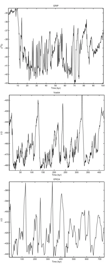
10 20 30 40 50 60 70 80 90 100 −43 −42 −41 −40 −39 −38 −37 −36 −35 Time (kyr) δ 18O GRIP 50 100 150 200 250 300 350 400 −480 −470 −460 −450 −440 −430 −420 Time (kyr) δ D Vostok 100 200 300 400 500 600 700 −440 −430 −420 −410 −400 −390 −380 Time (kyr) δ D EPICA
Fig. 1. Time-series of temperature proxies. From top to bottom for: Grip (δ18Oin ‰), Vostok and EPICA (δD in ‰). Time is expressed in kyr.
Materials and methods
A modified version of EMD method, developed in Huang et al. (1998), has been used to produce a linear decomposition of series in non-linear modes, the so-called Intrinsic Mode Functions (IMF). IMFs represent partial Hilbert transforms of the signal, and so they posses special properties such as the smoothness in both frequency and amplitude modula-tion. The EMD method is based on the existence of local time-scales of the data, what gives a precise meaning to local frequencies and allows to remove spurious harmonics (typ-ical in Fourier analysis) in the representation of non-linear and non-stationary signals (Coughlin and Tung, 2004). The essence of EMD is to empirically identify oscillatory modes in the data by means of their local extrema. Such a decom-position is based in three assumptions (Huang et al., 1998, 2003; Wu and Huang, 2003): (1) the signal has at least two extrema -one maximum and one minimum; (2) the character-istic local time scale is defined by the time interval between two consecutive extrema; and (3) if the data were totally free of extrema but contained only inflection points, then the sig-nal can be obtained by the integration of the components.
For this work we have used a MatLab implementation of the algorithm, provided by Patrick Flandrin and collaborators (Rilling et al., 2003; Flandrin et al., 2004). The code can be retrieved at the following URL: http://perso.ens-lyon.fr/ patrick.flandrin/emd.html.
The series under study are represented in Fig. 1. They are GRIP 100 ky before present (BP) series, Vostok 400 ky BP series, and Epica 741 ky BP series (all downloaded at http://www.ncdc.noaa.gov/paleo/data.html). GRIP series de-scribes the time evolution of the differences in
concentra-tion of the oxigen isotope (18O) (Saltzman, 2002) δ18O
(ex-pressed in parts per thousand, ‰), which is directly propor-tional to the zonal temperature (Dahl-Jensen et al., 1998; Landais et al., 2004). These data have uneven time resolu-tion, ranging from 1.3 years for the most recent records to 172 years for the oldest one (Dansgaard et al., 1993; Landais et al., 2003). Vostok time series (Petit et al., 1999) describes the time evolution of the differences in concentration of deu-terium (D) (Saltzman, 2002) δD (expressed in parts per thou-sand, ‰) in a time span of 422 766 years. The time resolution of the data is 17 years for the earliest records and 664 yr in the most distant ones. Epica (EPICA community members, 2004) time series describes the time evolution of the concen-tration of δD (expressed in parts per thousand, ‰) in a time span of 741 kyr BP. The time resolution is 68.5 yr for the ear-liest records and 5421 yr for the most distant ones. Previous to the extraction of the IMF’s we pre-process the time series by calculating a uniform sampling surrogate of lower reso-lution. This surrogate is obtained by sampling the different series with boxes of 200 years for Grip, 500 years for Vostok and 3000 years for Epica, associating to each box a represen-tative: the average of the points contained in that box inter-val. Such an average-downsampling acts much as a low-pass
filter and diminishes fluctuations1. Uniformly sub-sampling
the series is not really necessary, as EMD should also work on the non-uniform series; however, this pre-process is con-venient in order to give more stability to the procedure of IMF extraction, so reducing the number of iterations neces-sary to obtain each IMF. In fact, this uniform sampling is necessary to compare the IMFs coming from different time series.
Not all the IMFs directly emerging from EMD can be con-sidered as physically significant. As a matter of fact, there must be some degree of noise contaminating the sample. We will assume that series are affected by additive, white noise. When a signal is affected by other types of noise (e.g. red noise), this will appear as an additional IMF component in the decomposition, which will utterly need to be interpreted. As EMD is a linear decomposition, we can assume that, af-ter decomposition, each empirical IMF is the sum of a signal IMF plus a noise IMF. As noise contributes with constant amplitude at all frequencies, noise IMFs have the same, con-stant amplitude and frequency ranges coincident with those of the associated signal IMFs. As far as noise IMF ampli-tude is significantly smaller than signal IMF ampliampli-tude, we can consider the empirical IMF to be physically meaning-ful. Contrarily, when noise IMF amplitude is larger than signal IMF amplitude the noise will mask the structure of the signal IMF and hence the empirical IMF must be dis-carded. We can reasonably assume that the first empirical IMF, which comprises the highest frequencies, is completely corrupted by noise and we take its amplitude level as a ref-erence of the amplitude of noise IMFs. So, we establish the following criterion to consider an empirical IMF physically significant: the amplitude of that IMF must be at least one third of the maximum amplitude of the first (i.e. highest fre-quency) IMF. Notice that, contrarily to noise, physical sig-nals (for instance, finite variation sigsig-nals) usually have am-plitudes which increase as frequency decreases (what can be observed, for instance, when the power-spectrum is evalu-ated and a power-law decay is observed). Hence, as we con-sider following orders in the IMF decomposition frequency decreases and signal IMF amplitude increases, so they even-tually become significantly larger than those of noise and the empirical IMF can then considered as reliable. This does not mean that as frequency decreases only physically sig-nificant empirical IMFs happen: sometimes, an additional, completely spurious IMF appears, with no signal contribu-tion. These can be recognized as purely noise IMFs precisely because of their small amplitude. Notice also that our crite-rion to select IMFs has a direct physical interpretation: the square of the amplitude of each IMF gives its energy; hence, small amplitudes mean low energy contribution to the whole signal. In order to keep the total energy of the signal, we ac-cumulate all noise-dominated IMFs and the lowest frequency
1In fact, this downsampling could be considered as cutting the
302 J. Sol´e et al.: EMD to correlate paleoclimatic TS 20 40 60 80 100 −1 0 1 Time (kyr) δ 18 O 20 40 60 80 100 −2 −1 0 1 Time (kyr) δ 18 O 20 40 60 80 100 −2 0 2 Time (kyr) δ 18 O 20 40 60 80 100 −1 0 1 Time (kyr) δ 18 O 20 40 60 80 100 −1 −0.50 0.5 Time (kyr) δ 18 O 20 40 60 80 100 −2 0 2 Time (kyr) δ 18 O 20 40 60 80 100 −40 −39 −38 Time (kyr) δ 18 O GRIP IMFs
Fig. 2. IMFs of GRIP series, from highest (upper left) to lowest frequencies (down). Time is expressed in kyr.
IMF (the trend, as it does not oscillate) in a remaining term. Hence, we produce a reduced IMF decomposition, formed by the physically significant, oscillating IMFs.
Once the reduced set of IMFs for each signal has been ob-tained, we can calculate the phase difference between two IMFs belonging to two different series, in order to assess
their degree of synchronization. Given two time series, s1(t )
and s2(t ), their reduced IMF decompositions read:
s1(t ) =X n
c1n(t ); s2(t ) =X m
c2m(t ) (1)
where cn1(t ), c2m(t )are the IMFs of each series (we follow
the convention of designating the remaining term as the last IMF). In order to evaluate the phase differences of two given
IMFs, cn1(t )and c2m(t ), we need first to define their local
fre-quencies. This can be done by means of the Hilbert trans-form of each mode. The Hilbert transtrans-form of a function Rudin (1987) creates a complex completion of it, shifting
its phase by 90 degrees. Hence, if an IMF cn(t )can be
ex-pressed in terms of its amplitude an(t )and phase evolution
θn(t )as cn(t )=an(t )cos θn(t ), the Hilbert transform of cn(t ),
denoted by H cn(t ), verifies that H cn(t ) = an(t )sin θn(t ).
We can hence use Hilbert transforms to isolate the amplitude
an(t )and the phase evolution θn(t )of each mode cn(t ), and
obtaining from them the phase differences between two given
modes. Let us first introduce the set of complex IMFs c1n(t )
and c2m(t ), given by:
c1n(t ) ≡ c1n(t ) + H c1n(t ) = an1(t ) eiθ1,n(t )
c2m(t ) ≡ c2m(t ) + H cm2(t ) = a2m(t ) eiθ2,m(t ) (2)
We are interested in the phase velocity, that is, the relative
phase speed 1θnm(t )=θ1,n(t )−θ2,m(t ). It can be derived
from the following expression:
ei1θnm(t ) = c
1
n(t ) · (c2m(t ))∗
|c1n(t )||c2m(t )| . (3)
We define the real projection of the phase shift, δnm(t ), as:
δnm(t ) ≡ cos(1θnm(t )) = Re(ei1θnm(t )) (4)
Finally, we will take the variance of δnm(t )(var[δnm(t )]) as
a global indicator of constant phase shift between two given
IMFs n and m. As a matter of fact, var[δnm(t )] =0 means
constant phase shift, while var[δnm(t )] ≥0.5 for modes with
very different local frequencies. We fix a compromise
thresh-old of 0.3 for var[δnm(t )]to detect couples of modes having
constant phase shift over a reasonable long time span. The inter-series phase shift of modes is a good estimator of the degree of closeness of the modes and gives a useful informa-tion on the oscillating pattern of the couple.
100 200 300 400 −5 0 5 Time (kyr) δ D 100 200 300 400 −5 0 5 Time (kyr) δ D 100 200 300 400 −5 0 5 Time (kyr) δ D 100 200 300 400 −20 0 20 Time (kyr) δ D 100 200 300 400 −20 0 20 40 Time (kyr) δ D 100 200 300 400 −10 0 10 Time (kyr) δ D 100 200 300 400 −5 0 5 Time (kyr) δ D 100 200 300 400 −466 −464 −462 Time (kyr) δ D Vostok IMFs of can all appears. ing beha phase 10 graphs o phase Discussion Using position
Fig. 3. IMFs of Vostok series, from highest (upper left) to lowest frequencies (down right). Time is expressed in kyr.
200 400 600 −10 0 10 Time (kyr) δ D 200 400 600 −10 0 10 Time (kyr) δ D 200 400 600 −20 0 20 Time (kyr) δ D 200 400 600 −20 0 20 Time (kyr) δ D 200 400 600 −4 −2 0 2 4 Time (kyr) δ D 200 400 600 −421 −420 −419 −418 −417 Time (kyr) δ D
Epica IMFs that
lo sometimes lem series: disturb ef tw Recently ferent 2003). be longer able adv tion domain compositon
Fig. 4. IMFs of Epica series, from highest (upper left) to lowest frequencies (down right). Time is expressed in kyr.
2 Results
We have decomposed the three time series of data into their IMFs. The decomposition separates modes from those with local high frequencies to the ones with low local frequen-cies. The lowest frequency mode (comprising the empiric lowest frequency mode plus the physically non-significant modes, as explained before) is always an almost DC compo-nent, which does not arrive to create a full oscillation so it can be interpreted as the series trend. As discussed before, we expect that low frequency IMFs can be associated to physi-cal forcings common to all the series, while high-frequency IMFs will likely depend on noise and proxy-specific
pro-cesses. As observed in the figures, local periods are not constant but for each fixed IMF they are contained within different, non-overlapping ranges. The IMFs of GRIP se-ries are shown in the Fig. 2, with oscillation patterns periods of about 100 kyr (last component), 30–50 kyr (6th mode),
∼15 kyr (5th mode), and ∼5 kyr (4th mode). The IMFs of
Vostok series are presented in the Fig. 3; there the local pe-riods range from 80–120 kyr observed in the 6th mode, 40– 50 kyr in the 5th mode, and 20–30 kyr in the 4th mode. In Epica (Fig. 4) the IMFs exhibit local periods ranging from 80–120 kyr for the 4th mode, 40–50 kyr for the 3rd mode, and 20–30 ky for the 2nd mode.
304 J. Sol´e et al.: EMD to correlate paleoclimatic TS
a-1)
0 10 20 30 40 50 60 70 80 90 100 −4 −2 0 2 4 δ 18 O Time (kyr) Grip−Vostok 0 10 20 30 40 50 60 70 80 90 100−20 −10 0 10 20 δDa-2)
10 20 30 40 50 60 70 80 90 100 −0.6 −0.4 −0.2 0 0.2 0.4 0.6 0.8 Grip−Vostok Time (kyr) δb-1)
0 10 20 30 40 50 60 70 80 90 100 −4 −2 0 2 4 δ 18O Time (kyr) Grip−Epica 0 10 20 30 40 50 60 70 80 90 100−20 −10 0 10 20 δDb-2)
10 20 30 40 50 60 70 80 90 100 0.1 0.2 0.3 0.4 0.5 0.6 0.7 0.8 0.9 Time (kyr) δ Grip−Epicac-1)
0 50 100 150 200 250 300 350 400 −20 0 20 δD Time (kyr) Vostok−Epica 0 50 100 150 200 250 300 350 400 −50 0 50 δDc-2)
50 100 150 200 250 300 350 400 0 0.1 0.2 0.3 0.4 0.5 0.6 0.7 0.8 0.9 Vostok−Epica Time (kyr) δFig. 5. (a) Grip 6th mode and Vostok 5th mode for 100 ky period (top) and the associated δ65(t )(bottom) (b) Grip 6th mode and Epica 3th
mode for 100 ky period (top) and the associated δ63(t )(bottom) (c) Vostok 6th mode and Epica 4th mode for 400 ky period (top) and the
associated δ64(t )(bottom).
for all possible couples of IMFs from two series, that is, to obtain the matrices of variance between IMFs of couples of series. As mentioned before, we select those couples of modes having variance less than 0.3, as they are more likely to exhibit lasting periods of synchronization. In Fig. 5a-1 we present joints graphs of IMFs from Grip and Vostok series, restricted to the common time span of 100 kyrs BP (6th mode
of Grip and 5th of Vostok). In Fig. 5a-2, δ65(t )is shown. We
can observe the phase coincidence (δ65(t ) ∼ 1) for almost
all the time, except in the last 10 ky where an opposite phase appears. We can also observe the common local period rang-ing from 40 to 50 kyr. For the couple Grip-Epica ( 5b-1) the behavior is similar to the previous case, having a coincident phase in the first 90 kyr, and an opposite phase at the last 10 kyr, as seen in Fig. 5b-2. In Fig. 5c-1, the joint graphs of Vostok and Epica series are shown; phases coincide over
practically all the period, as shown in Fig. 5c-2. The phase ranges between the 120 kyr to 80 kyr period.
3 Discussion
Using an objective method as the Empirical Mode Decom-position (EMD), we have separated different oscillation pat-terns composing the selected three paleoclimatic time series. The EMD method allows to relate and to compare differ-ent time series, despite precise timings, just by considering their common characteristics. A word of warning on EMD should be introduced here. Although the EMD method has well-founded theoretical roots, some problems limit its per-formance in practice (Huang et al., 1998, 2003). Two are the main limitations. The first one is the difficulty to perform
a clean separation in IMFs when their local frequencies are too close. This partially happens in some of our IMFs and for that reason the correlations between individual IMFs are a bit lowered, as a fraction of the IMF energy of a given mode is sometimes attributed to another close IMF. The second prob-lem with EMD has to do with domain boundaries of the time series: the two endings (beginning and end of the time span) disturb the local frequency for around half a cycle, and this effect also lowers the mutual correlations, specially when two series with very different time sampling are compared. Recently, these two difficulties have been discussed and dif-ferent ways to solve them have been proposed (Huang et al., 2003). In spite of these problems, the method has proved to be rather robust and so it is guaranteed that, at least for the longer features, EMD will produce a decomposition reason-able enough to give an interpretation of the results. The main advantage of using EMD lies in the fact that the decomposi-tion is peformed in the time domain instead of the frequency domain typical of Fourier methods. This time domain de-compositon allows to obtain an instantaneous frequency at each time instant and then to locally compare the instant fre-quencies of two points from two diferent time series. Those instantaneous frequencies allow for instance, to identify the starting and finishing intants of relevant events. Frequency domain decomposition methods derived from Fourier analy-sis, on the contrary, do not allow to associate a characteristic frequency at each point in the time-series and consequently to compare points of two different series, except in the case where the two series are stationary.
The results of the different series decomposition show common, regular oscillation patterns (for medium and low frequencies). Correlating series by pairs we have observed the presence of two common oscillation patterns (for Grip, Vostok and Epica), one with local periods in the range from 80 to 120 ky, and other ranging from 30 to 50 ky. This coinci-dences could be interpreted as the effect of a non-local com-mon forcing mechanism, but the weak time dependence of the local phase (as can be seen in the coupled modes of three series) and the growing period of oscillation with the time, seems to indicate that the effect on the temperature proxies is strongly non-linear. This seems to suggest that although a pe-riodic non-local forcing mechanism as Milankovitch forcing mechanism (Milankovitch, 1941) can act over well-defined periods, the system response may show non-linear relations, like power-law responses (Huybers and Curry, 2006). Be-tween all the non-linear coupling mechanisms that can pro-duce such patterns, the stochastic resonance is cited in the literature as a plausible phenomena that can trigger abrupt changes or climate oscillations (Gammaitoni et al., 1998; P.V´elez-Belch´ı et al., 2001; Alley et al., 2001; Ganopolski and Rahmstorf, 2002; Sol´e et al., 2007). It has also been ar-gued that a possible cause mechanism that forces the change stadial-interstadial can be found in the change of the At-lantic thermohaline circulation (Clark et al., 2002; Rahm-storf, 2002; Stocker, 2002; Alley et al., 2003). Other
hy-potesis for that change in such a non-constant phase oscilla-tion can be found in a tidal forcing mechanism (Keeling and Whorf, 1997, 2000).
We have seen that the series of temperature proxies stud-ied here have their own particularities and different origins but are subjected to the same climatic forcings, and con-sequently their dynamic behavior present common aspects. The use of EMD allows us to compare different series, so giving a powerful method to extract the common behavior of the series. Using this method we can extract precise in-formation about local mechanisms in different scales and to decide if the supposed driving forcings are the main influ-encing mechanism in the time-scales considered or the sys-tem has a more complex behavior in such time periods. This can be a first step for to study from a objective point of view the common patterns of given paleoclimatic time series, but more detailed analysis, as well as improvements in the EMD methodology, should be undertaken in the future in order to give more strength to the hypotheses presented here. The in-troduction of additional temperature proxies would also help to extract more meaningful intrinsic modes.
Another different branch of research concerns the adjust-ment of time-schedules: if two IMFs are suspected to be co-incident but they show some phase difference due to timing errors, it would be possible to re-define the time sampling of one series according to the other series sampling by us-ing an invertible function t →f (t ) so that phase shifts
van-ish, i.e., if we trust the time schedule for c1n(t )we look for
f (t )such that cm,f2 (t )≡c2m(f (t )) verifies δnm,f(t )=0. The
ability of IMFs to separate common forcings from particu-lar relaxation cycles will enable to refer the time labeling of the different series to a fixed reference, enhancing the degree of confidence about event synchronization. Further research should be enterprised in this direction.
Acknowledgements. AT is supported by Ramon y Cajal contract
from the Spanish Ministry of Education. JELL acknowledges partial financial support of contract REN2003-00185.
Edited by: L. Ferraris Reviewed by: two referees
References
Alley, R., Anandakrishnan, S., and Jung, P.: Stochastic resonance in the North Atlantic, Paleoceanography, 16, 190–198, 2001. Alley, R., Marotzke, J., Nodhaus, W., Overpeck, J., Peteet, D. M.,
Pielke, R., Pierrehumbert, R., Rhines, P., Stocker, T., Talley, L., and Wallace, J.: Abrupt Climate Change, Science, 299, 2005– 2010, 2003.
Bond, G., Broecker, W., Johnsen, S., McManus, J., Labeyrie, L., Jouzel, J., and Bonani, G.: Correlations between climate records from North Atlantic sediments and Greenland ice, Nature, 365, 143–147, 1993.
Broecker, W.: Massive iceberg discharges as triggers for global cli-mate change, Nature, 372, 421–424, 1994.
306 J. Sol´e et al.: EMD to correlate paleoclimatic TS
Clark, P., Pisias, N., Stocker, T., and Weaver, A.: The role of the thermohaline circulation in abrupt climate change, Nature, 415, 863–869, 2002.
Coughlin, K. and Tung, K.: 11-year solar cycle in the stratosphere extracted by the empirical mode decomposition method, Adv. Space Res., 34, 323–329, 2004.
Cronin, T.: Principles of Paleoclimatology, Columbia University press, New York, 1999.
Cruz, F., Burns, S., karmann, I., Sharp, W., Vuille, M., Cardoso, A., Ferrari, J., Dias, P. S., and Jr, O.: Insolation-driven changes in at-mospheric circulation over the past 116 000 years in subtropical Brazil, Nature, 434, 63–66, 2005.
Dahl-Jensen, D., Mosegaard, K., Gundestrup, N., Clow, G. D., Johnsen, S. J., Hansen, A. W., and Balling, N.: Past Tempera-tures Directly from the Greenland Ice Sheet, Science, 282, 268– 279, 1998.
Dansgaard, W., Johnsen, S., Clausen, H., Dahl-Jensen, D., Gundestrup, N., Hammer, C., Hvidberg, C., Steffensen, J., Sveinbj¨ornsd´ottir, A., Jouzel, J., and Bond, G.: Evidence for general instability of past climate from a 250 kyr ice-core record, Nature, 264, 218–220, 1993.
El-Askary, H., Sarkar, S., Chiu, L., Kafatos, M., and El-Ghazawi, T.: Rain gauge derived precipitation variability over Virginia and its relation with the El Nino southern oscillation. Adv. Space Res., 33, 338–342, 2004.
EPICA community members: Eight glacial cycles from an antarctic ice core, Nature, 429, 623–628, 2004.
Flandrin, P., Rilling, G., and Gonc¸alv`es, P.: Empirical mode de-composition as a filterbank, Signal Processing Letters, IEEE, 11, 112–114, 2004.
Gammaitoni, L., H¨anggi, P., Jung, P., and Marchesoni, F.: Stochas-tic resonance, Rev. Modern Phys., 70, 223–287, 1998.
Ganopolski, A. and Rahmstorf, S.: Abrupt glacial climate changes due to stochastic resonance, Phys. Rev. Lett., 88, 38 501–38 504, 2002.
Gloersen, P. and Huang, N.: Comparison of interannual intrinsic modes in hemispheric ice covers and other geophysical parame-ters, IEEE Transactions in Gosciences and Remote Sensing, 41, 1062–1074, 2003.
Heinrich, H.: Origin and consequences of cyclic ice rafting in the northeast Atlantic Ocean during the past 130 000 years, Quat. Res., 29, 142–152, 1998.
Hemming, S.: Heinrich events: massive late Pleistocene detritus layers of the North Atlantic and their global climate imprint, Rev. Geophys., 42, 1–43, 2004.
Hu, Z. and Wu, Z.: The intensification and shift of the annual North Atlantic Oscillation in a global warming scenario simu-lation, Tellus, 56, 112–124, 2004.
Huang, N., Shen, Z., Long, S., Wu, M., Shih, H., Zhen, Q., Yen, N., Tung, C., and Liu, H.: The empirical mode descomposition and the Hilbert spectrum for nonlinear and non-stationary time series analysis, Proc. R. Soc. London, 454, 903–995, 1998.
Huang, N., Wu, M., Long, S., Shen, S., Qu, W., Gloersen, P., and Fan, K.: A confidence limit for the empirical mode decompo-sition and Hilbert spectral analysis, Proc. R. Soc. London, 459, 2317–2345, 2003.
Huybers, P. and Curry, W.: Links between annual, Milankovitch and continuum temperature variability, Nature, 441, 329–332, 2006.
J´anosi, I. M. and M¨uller, R.: Empirical mode decomposition and correlation properties of long daily ozone records, Phys. Rev. E, 71, 1597–1611, 2006.
Keeling, C. and Whorf, T.: Possible forcing of global temperature by the oceanic tides, Proceedings of the National Academy of Sciences, 94, 8321–8328, 1997.
Keeling, C. and Whorf, T.: The 1.800-year oceanic tidal cycle: A possible cause of rapid climate change, Proceedings of the Na-tional Academy of Sciences, 97, 3814–3819, 2000.
Knutti, R., Fl¨uckiger, J., Stocker, T., and Timmermann, A.: Strong hemispheric coupling of glacial climate through freshwater dis-charge and ocean circulation, Nature, 430, 851–856, 2004. Landais, A., Barnola, J. M., Masson-Delmotte, V., J. Jouzel, J. C.,
Caillon, N., Huber, C., Leuenberger, M., and Johnsen, S. J.: A continuous record of temperature evolution over a sequence of Dansgaard-Oeschger events during Marine Isotopic Stage 4 (76 to 62 kyr BP), Geophys. Res. Lett., 31, 4563–4572, 2004. Landais, A., Chapellaz, J., Delmotte, M., Jouzel, J., Blunier, T.,
Bourg, C., Caillon, N., Cherrier, S., Malaiz´e, B., Masson-Delmotte, V., Raynaud, D., Schwander, J., and Steffensen, J.: A tentative reconstruction of the last interglacial and glacial incep-tion in Greenland based on new gas measurements in the Green-land Ice Core Project (GRIP) ice core, J. Geophys. Res., 108, 4563–4572, 2003.
Lin, Z. and Wang, S.: EMD analysis of solar insolation, Meteorol. Atmos. Phys., 93, 123–128, 2006.
Milankovitch, M.: Canon of insolation and ice-age problem, Royal Serb Acad, 1941.
Molla, K., Sumi, A., and Rahman, M.: Analysis of Temperature Change under Global Warming Impact using Empirical Mode Decomposition, Int. J. Information Technol., 3, 131–139, 2006. Morgan, V., Delmotte, M., van Ommen, T., Jouzel, J., Chapellaz, J., Woon, S., Masson-Delmotte, V., and Raynaud, D.: Relative tim-ing of Deglacial Climate Events in Antarctica and Greendland, Science, 297, 1862–1864, 2002.
Pahnke, K. and Zahn, R.: Southern Hemisphere Water Mass Con-version Linked with North Atlantic Climate Variability, Science, 307, 1741–1746, 2005.
Petit, J., Jouzel, J., Raynaud, D., Barkov, N., Barnola, J., Basile, I., Bender, M., Chappellaz, J., Davis, J., Delaygue, G., Delmotte, M., Kotlyakov, V., Legrand, M., Lipenkov, V., Lorius, C., P´epin, L., Ritz, C., Saltzman, E., and Stievenard, M.: Climate and at-mospheric history of the past 420,000 years from the vostok ice core, antarctica, Nature, 399, 429–436, 1999.
P.V´elez-Belch´ı, Alvarez, A., Colet, P., and Tintor´e, J.: Stochastic resonance in the thermohaline circulation, Geophys. Res. Lett., 28, 2053–2056, 2001.
Rahmstorf, S.: Ocean circulation and climate during the past 120 000 years, Nature, 419, 207–214, 2002.
Rahmstorf, S. (2003). Timing of abrupt climate change: A precise clock. Geophysical Research Letters, 30:17–1–17–4.
Rilling, G., Flandrin, P., and Gonc¸alv`es, P.: On empirical mode de-composition and its algorithms. Technical report, UMR,INRIA, France. IEEE-EURASIP Workshop on Nonlinear Signal and Im-age Processing.Workshop Report, 2003.
Rudin, W.: Real and Complex Analysis, Mc Graw Hill, New York, USA, 1987.
Saltzman, B.: Dynamical Paleoclimatology, Academic Press, 2002.
Sinclair, S. and Pegram, G.: Empirical Mode Decomposition in 2-D space and time: a tool for space-time rainfall analysis and now-casting, Hydrol. Earth Syst. Sci., 9, 127–137, 2005.
Sol´e, J., Turiel, A., and Llebot, J.: Classification of Dansgaard-Oeschger climatic cycles by the application of similitude signal processing, Phys. Lett. A, in press, 2007.
Stocker, T.: North-south connections, Science, 297, 1814–1815, 2002.
Wu, Z. and Hu, C. K.: Empirical mode decomposition and synchro-gram approach to cardiorespiratory synchronization, Phys. Rev. E, 73, 1597–1611, 2006.
Wu, Z. and Huang, N.: A study of the characteristics of white noise using the empirical mode decomposition method, Proc. R. Soc. London, 460, 1597–1611, 2003.