Gap filling and noise reduction of unevenly sampled data by means of the Lomb-Scargle periodogram

(1)

HAL Id: hal-00304012

https://hal.archives-ouvertes.fr/hal-00304012

Submitted on 4 Mar 2008

HAL is a multi-disciplinary open access

archive for the deposit and dissemination of sci-entific research documents, whether they are pub-lished or not. The documents may come from teaching and research institutions in France or abroad, or from public or private research centers.

L’archive ouverte pluridisciplinaire HAL, est destinée au dépôt et à la diffusion de documents scientifiques de niveau recherche, publiés ou non, émanant des établissements d’enseignement et de recherche français ou étrangers, des laboratoires publics ou privés.

Gap filling and noise reduction of unevenly sampled

data by means of the Lomb-Scargle periodogram

K. Hocke, N. Kämpfer

To cite this version:

K. Hocke, N. Kämpfer. Gap filling and noise reduction of unevenly sampled data by means of the Lomb-Scargle periodogram. Atmospheric Chemistry and Physics Discussions, European Geosciences Union, 2008, 8 (2), pp.4603-4623. �hal-00304012�

(2)

ACPD

8, 4603–4623, 2008

Gap filling and noise reduction K. Hocke and N. K ¨ampfer

Title Page Abstract Introduction Conclusions References Tables Figures ◭ ◮ ◭ ◮ Back Close Full Screen / Esc

Printer-friendly Version Interactive Discussion Atmos. Chem. Phys. Discuss., 8, 4603–4623, 2008

www.atmos-chem-phys-discuss.net/8/4603/2008/ © Author(s) 2008. This work is distributed under the Creative Commons Attribution 3.0 License.

Atmospheric Chemistry and Physics Discussions

Gap filling and noise reduction of

unevenly sampled data by means of the

Lomb-Scargle periodogram

K. Hocke and N. K ¨ampfer

Institute of Applied Physics, University of Bern, Switzerland

Received: 25 January 2008 – Accepted: 4 February 2008 – Published: 4 March 2008 Correspondence to: K. Hocke (klemens.hocke@mw.iap.unibe.ch)

(3)

ACPD

8, 4603–4623, 2008

Printer-friendly Version Interactive Discussion

Abstract

The Lomb-Scargle periodogram is widely used for the estimation of the power spectral density of unevenly sampled data. A small extension of the algorithm of the Lomb-Scargle periodogram permits the estimation of the phases of the spectral components. The amplitude and phase information is sufficient for the construction of a complex 5

Fourier spectrum. The inverse Fourier transform can be applied to this Fourier spec-trum and provides an evenly sampled series (Scargle,1989). We are testing the pro-posed reconstruction method by means of artificial time series and real observations of mesospheric ozone, having data gaps and noise. For data gap filling and noise reduction, it is necessary to modify the Fourier spectrum before the inverse Fourier 10

transform is done. The modification can be easily performed by selection of the rele-vant spectral components which are above a given confidence limit or within a certain frequency range. Examples with time series of lower mesospheric ozone show that the reconstruction method can reproduce steep ozone gradients around sunrise and sunset and superposed planetary wave-like oscillations observed by a ground-based 15

microwave radiometer at Payerne.

1 Introduction

Atmospheric data are often unevenly sampled due to spatial and temporal gaps in net-works of ground stations, radiosondes, and satellites. Many measurement techniques such as lidar, solar UV backscatter, occultation depend on weather, solar zenith angle, 20

or constellation geometry and cannot provide continuous data series. Unevenly sam-pled data have one advantage since aliasing effects at high frequencies are reduced, compared to evenly sampled data (Press et al.,1992).

There are several approaches to come over with undesired data gaps: linear and cubic interpolation and triangulation (appropriate for small gaps), spherical harmonics 25

(4)

ACPD

8, 4603–4623, 2008

Printer-friendly Version Interactive Discussion and data assimiliation of observations into atmospheric general circulation models.

At-mospheric parameters often have periodic oscillations due to forcing processes within the dynamical system of Sun, atmosphere, ocean, and soil. Thus, gap filling by spectral methods can also be considered as an efficient tool.

Adorf (1995) performed a very brief and valuable survey on available interpolation 5

methods for irregularly sampled data series in astronomy.Kondrashov and Ghil(2006) describe the application of singular spectrum analysis for spatio-temporal filling of miss-ing points in geophysical data sets. The leadmiss-ing orthogonal eigenvectors of the lag-covariance matrix of data series are utilized for iterative gap filling. Ghil et al. (2002) give a detailed review on advanced spectral methods for reconstruction of climatic time 10

series (e.g. singular spectrum analysis, maximum entropy method, multitaper method). The review of Ghil et al. (2002) does not mention the Lomb-Scargle periodogram which provides the least-squares spectrum of unevenly sampled data series (Lomb,

1976; Scargle, 1982; Press et al., 1992). The Lomb-Scargle periodogram reduces to the Fourier transform in case of evenly sampled data. In presence of data gaps, 15

the sine and cosine model functions are orthogonalized by additional phase factors (Lomb, 1976). Scargle (1989) investigated the reconstruction of unevenly sampled time series by application of the Lomb-Scargle periodogram and subsequent, inverse Fourier transform. The potential of the study ofScargle(1989) for gap filling of atmo-spheric data sets has not been recognized yet, maybe because the article has been 20

published in an astronomical journal. Another reason is that most available computer programs of the Lomb-Scargle periodogram solely derive the spectral power density but not the phase or the complex Fourier spectrum.Hocke(1998) modified the Lomb-Scargle algorithm (Fortran program “period.f”) ofPress et al.(1992) in such a way that amplitudes and phases are returned as functions of frequency and tested the program 25

by means of artificial time series. The modified algorithm has been applied in various studies, e.g. for estimation of amplitudes and phases of tides, planetary waves, and gravity waves in the mesosphere and lower thermosphere, and for investigation of en-ergy dissipation rates in the auroral zone (Nozawa et al., 2005; Altadill et al., 2003;

(5)

ACPD

8, 4603–4623, 2008

Ford et al.,2006;Hall et al.,2003).

The present study continues the basic idea ofScargle(1989) and utilizes the Lomb-Scargle periodogram for reconstruction of time series. We explain the derivation of the complex Fourier spectrum from the Lomb-Scargle periodogram (Sect. 2). The com-plex Fourier spectrum should be reduced to its relevant spectral components before 5

the inverse Fourier transform yields the equally spaced time series without gaps and without noise. The reconstruction method is tested with synthetic data and with real observations of lower mesospheric ozone (Sect. 3). Particularly, the tests with time series of lower mesospheric ozone show that the reconstruction method is not only appropriate for gap filling. The reconstruction method also supports the interpretation 10

of the data and retrieves the regular daily change of lower mesospheric ozone with a high temporal resolution which is required around sunset and sunrise.

2 Data analysis

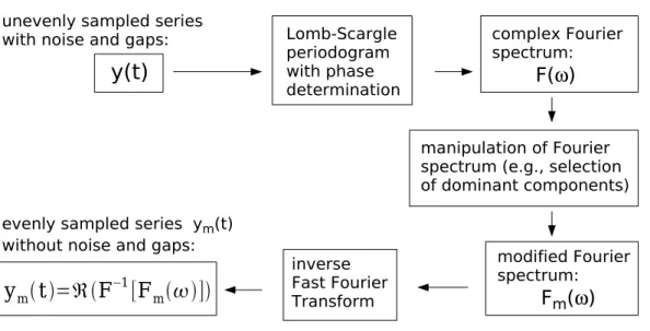
The flow chart of the data analysis for reconstruction of data gaps and noise reduction is illustrated in Fig. 1. In the following, we explain the principle of the Lomb-Scargle 15

periodogram. Special emphasis is put on the construction of a Fourier spectrum which is used for the inverse Fourier transform from the frequency domain back to the time domain. The selection of relevant spectral components has not been considered by

Scargle(1989). This idea is related to the selection of principal components or leading orthogonal eigenfunctions of the lag-covariance matrix for filling of data gaps ( Kon-20

drashov and Ghil,2006).

2.1 Lomb-Scargle periodogram

The Lomb-Scargle periodogram is equal to a linear least-squares fit of sine and cosine model functions to the observed time seriesy(ti) which shall be centered around zero

(6)

ACPD

8, 4603–4623, 2008

Printer-friendly Version Interactive Discussion (Lomb,1976;Press et al.,1992).

y(ti) =a cos (ωti − Θ) + b sin (ωti − Θ) + ni; with i = 1, 2, 3, ..., N (1)

where y(t_i) is the observable at time t_i, a and b are constant amplitudes, ω is the angular frequency,ni is noise at timeti, and Θ is the additional phase which is required

for the orthogonalization of the sine and cosine model functions of Eq. (1) when the 5

data are unevenly spaced.

According to the addition theorem of sine and cosine functions, Eq. (1) can also be written as

y(ti) =A cos (ωti − Θ − φ) + ni; with φ = arctan (b, a) and A =

p

a2+_b2_. ₍₂₎

This writing style shows that a cosine function with amplitudeA and phase ϕ=Θ+φ 10

is fitted to the observed time series. For the construction of the Fourier spectrum we need both, amplitude and phase.

The power spectral densityP (ω) of the Lomb-Scargle periodogram is given by

P (ω) = 1 2σ2 R(ω)2 C(ω) + I(ω)2 S(ω) ! , (3) R(ω) ≡ N X i =1 y(t_i) cos (ωt_i _{− Θ),} (4) 15 I(ω) ≡ N X i =1 y(t_i) sin (ωt_i _{− Θ),} (5) C(ω) ≡ N X i =1 cos2(ωti − Θ), (6) S(ω) ≡ N X i =1 sin2(ωti − Θ). (7) (8)

(7)

ACPD

8, 4603–4623, 2008

Printer-friendly Version Interactive Discussion σ2 is the variance of the y series. The phase Θ is calculated with the four quadrant

inverse tangent Θ = 1 2arctan N X i =1 sin (2ωt_i), N X i =1 cos (2ωt_i) ! . (9)

Scargle(1982) presented this formula of Θ as the exact solution for orthogonalization of the sine and cosine model functions of Eq. (1) in case of unevenly sampled data 5

(P cos (ωt_i_{−Θ) sin (ωt}_i_−Θ)=0).

Equations (1–9) describe the Lomb-Scargle periodogram (Lomb, 1976; Scargle,

1982; Press et al., 1992; Bretthorst, 2001a). Scargle (1982) or Hocke (1998) ex-plained that the variables R and I are closely related with the amplitudes of Eq. (1) (a= q 2/NR/√C and b= q 2/NI/√S). 10

2.2 Construction of the complex Fourier spectrum

For calculation of the complex Fourier spectrum (as required for the FFT algorithm of the program language Matlab), the normalization of the spectral power density P (ω) of Eq. (3) is removed by multiplication of P with σ2 (variance of the y series). The amplitude spectrumA_{F T} is 15 AF T(ω) = r n 2σ 2_{P (ω),} ₍₁₀₎

wheren is the dimension of the complex Fourier spectrum F .

It is better to start the time vector witht1=0 (before calculation of the Lomb-Scargle

periodogram). Within the program period.f of Press et al. (1992), the phase is cal-culated with respect to the average time tave=(t1+tN)/2. The change of the phase

20

(8)

ACPD

8, 4603–4623, 2008

1989;Hocke,1998). The phaseϕ_{F T} of the complex Fourier spectrum (inclusive phase correctionωtave) is given by

ϕ_{F T} = arctan (I, R) + ωtave+ Θ. (11)

The real part of the Fourier spectrum is

RF T =AF T cosϕF T. (12)

5

The imaginary part of the Fourier spectrum is I_{F T} =_A

F T sinϕF T. (13)

The FFT-algorithm of the program language Matlab requires a complex vector F of such a format:

F = [complex(0, 0), complex(R_{F T}, I_{F T}), reverse[complex(R_{F T}, −IF T)]]. (14)

10

The first number is the mean of the time series (zero mean), then comes the complex spectrum, and finally the reverse, complex conjugated spectrum is attached.

For the frequency grid, we used an oversampling factor ofac=4 in order to have a small spacing of the frequency grid points . The frequencies are at

ω_j = 2π (tN− t1)ofac

j, with j = 1, 2, 3, ..,Nofac

2 . (15)

15

There are other small details, and the reader is referred to our Matlab program lspr.m which is an extension of the program period.f (Press et al.,1992) and which is provided as auxiliary material of the present study.

2.3 Reconstruction

Once the complex Fourier spectrum is in the right format, the data analysis is quite 20

(9)

ACPD

8, 4603–4623, 2008

Printer-friendly Version Interactive Discussion all spectral components with amplitudes below a certain confidence limit can be set

to zero, and/or spectral components within certain frequency bands can be easily re-moved. Thus, there are many possibilities for modifications of the time series in the frequency domain, and several examples are shown in the next section. The inverse Fourier transform of the modified Fourier spectrum Fm quickly provides the result in

5

the time domain (Fig. 1). The real part of F−1₍_F

m) is an evenly spaced time series

with reduced noise and composed by the selected spectral components. We have not investigated yet, but it is likely, that the phase information could be utilized for modifica-tion of the Fourier spectrum. For example, the phase spectrum may contain valuable information on phase coupling of atmospheric oscillations.

10

3 Results

3.1 Test with synthetic data

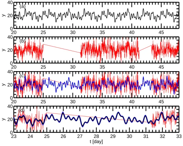
The periodic signal within the synthetic data series consist of 5 superposed sine waves with frequencies from 0.3 to 3 cycles/day. The time interval is 60 days long, and the sampling time is 20 min. A segment of the signal curve is shown in Fig.2a. Random 15

noise is added to the signal curve. The random noise is by a factor of 2.5 larger than the signals. The combined series of periodic signals, random noise, and data gaps are depicted in Fig. 2b. The series will be used for a test of data gap filling by the Lomb-Scargle periodogram.

For preparation, we subtract the arithmetic mean from the series of Fig.2b and mul-20

tiply the series with a Hamming window. Then we apply the data analysis as described by Fig. 1 and obtain the blue curve in Fig. 2c which is almost identical with the true signal curve (black line in Fig.2c). For the sake of a better comparison of the blue and the black line, Fig.2d shows a zoom of Fig.2c. Our data analysis successfully reduced the noise of the red line in Fig. 2b which was the input series and correctly filled the 25

(10)

ACPD

8, 4603–4623, 2008

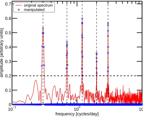
Printer-friendly Version Interactive Discussion The modification of the Fourier spectrum (Fig.1) is not mentioned byScargle(1989)

and is described in more detail by the amplitude spectra of Fig.3. The red line is the amplitude spectrum as obtained from the red time series of Fig. 2b by means of the Lomb-Scargle periodogram. The blue symbols denote the modified spectrum which is used for the inverse fast Fourier transform providing the blue line of Fig. 2c. All 5

spectral components with amplitudes smaller than the dashed horizontal line of Fig.3

are removed by setting their amplitudes to zero.

In case of geophysical data, confidence limits can be utilized for separation between relevant spectral components and noise. As already mentioned, more sophisticated methods of spectrum modification are also thinkable. In the following we give an ex-10

ample with real data, showing the consequence if the spectrum is not modified.

3.2 Test with observational data of lower mesospheric ozone

3.2.1 SOMORA ozone microwave radiometer

The stratospheric ozone monitoring radiometer (SOMORA) monitors the radiation of the thermal emission of ozone at 142.175 GHz. SOMORA has been developed at the 15

Institute of Applied Physics, University Bern. The instrument was first put into operation on 1 January 2000 and was operated in Bern (46.95 N, 7.44 E) until May 2002. In June 2002, the instrument was moved to Payerne(46.82 N, 6.95 E) where its operation has been taken over by MeteoSwiss. SOMORA contributes primary data to the Network for Detection of Atmospheric Composition Change (NDACC).

20

The vertical distribution of ozone is retrieved from the recorded pressure-broadened ozone emission spectra by means of the optimal estimation method (Rodgers,1976). A radiative transfer model is used to compute the expected ozone emission spectrum at the ground. Beyond 45 km altitude, the model atmosphere is based on monthly averages of temperature and pressure of the CIRA-86 climatology, adjusted to actual 25

ground values using the hydrostatic equilibrium equation. Either a winter or summer CIRA-86 ozone profile is taken as a priori. The retrieved profiles minimize a cost

(11)

func-ACPD

8, 4603–4623, 2008

Printer-friendly Version Interactive Discussion tion that includes terms in both the measurement and state space. The altitudeh is

fixed in both the forward and inverse models, and altitude-dependent information is ex-tracted from the measured spectra by reference to the used pressure profile. SOMORA retrieves the volume mixing ratio of ozone with less than 20% a priori contribution in the 25 to 65 km altitude range, with a vertical resolution of 8–10 km, and a time reso-5

lution (spectra integration time) of ∼30 min. More details concerning the instrument design, data retrieval, intercomparisons, and applications can be found in Calisesi

(2000), Calisesi (2003), Calisesi et al. (2005), Hocke et al. (2006), and Hocke et al.

(2007). Here, we use SOMORA measurements of ozone volume mixing ratio in the lower mesosphere ath=52 km having a time resolution of about 30 min.

10

3.2.2 Lower mesospheric ozone in summer and winter

A data segment with a length of 40 days and starting on 10 July 2004 is selected. The lower mesospheric ozone series of the SOMORA radiometer are depicted by the black line in Fig.4. Two major gaps appear around day 6.5 and day 12. If we apply the data analysis (Fig.1) without the modification of the spectrum, the red line is retrieved which 15

well captures the original series. However the noise is not reduced and the gaps are just filled by the arithmetic mean of the time series. This is certainly not desired but the example gives us some insight into the Lomb-Scargle periodogram method. The variance of the evenly sampled series (red line) minimizes at the locations of the data gaps.

20

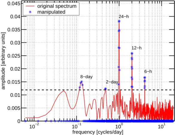
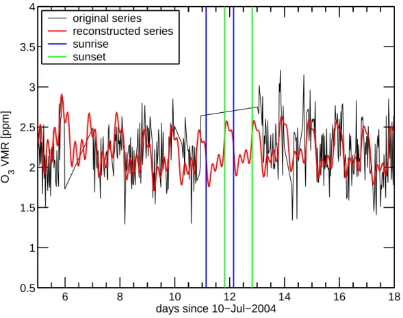
Reduction of the spectrum to its dominant spectral components seems to be neces-sary for an improved filling of the data gaps. Thus all spectral components with am-plitudes smaller than the 98%-confidence limit (dashed horizontal line) are set to zero in Fig.5where the full spectrum is shown by the red line, and the modified spectrum is given by the blue symbols. Application of the fast Fourier transform to the modified 25

spectrum yields the series of Fig.6. The red line is the reconstructed series which has been retrieved from the black, original series. The data gap around day 12 is well filled. The time points of sunrise and sunset are independently determined and are marked

(12)

ACPD

8, 4603–4623, 2008

Printer-friendly Version Interactive Discussion by blue and green vertical lines respectively. Due to fast recombination of atomic and

molecular oxygen after sunset, the ozone volume mixing ratio is larger during night-time. The reconstructed series well captures the regular daily variation. Additionally a planetary wave-like oscillation with a period of about 8 days is also present in the reconstructed series of Fig.6. If we go back to the spectrum in Fig.5, we see spec-5

tral components due to planetary wave-like oscillations (e.g. 8-day, 2-day) as well as the diurnal, semidiurnal, and 6-h components. Because of these periodic signals, the reconstruction by spectral methods yields good results in Fig.6.

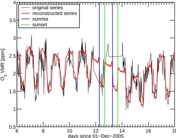
Finally the reconstruction method is applied to lower mesospheric ozone observed ath=52 km in winter (December 2005) by the SOMORA radiometer. The daily vari-10

ation of the red curve in Fig. 7 is different to Fig. 6, since the nights are longer in winter. Additionally, planetary wave activity is usually stronger in winter. However the red reconstructed series of Fig.7well represent the daily variations and the planetary wave-like oscillations in winter too. The major gap around day 13 is well filled by the Lomb-Scargle reconstruction method. We like to emphasize that the reduction of noise 15

and the filling of data gaps are valuable for a better recognition of basic processes such as the impact of sunrise and sunset on lower mesospheric ozone. A good estimate of the regular daily variation of lower mesospheric ozone with a high temporal resolution is needed for analysis of gravity wave-induced short-term variance of ozone (Hocke

et al., 2006). Digital filtering of the ozone series in the time domain cannot correctly 20

distinguish between sudden changes of the ozone distribution around the solar termi-nator and gravity wave-induced short-term fluctuations of ozone. A reconstruction by means of spectral methods can solve this problem (Fig.7).

4 Conclusions

The reconstruction of unevenly sampled data series with data gaps has been per-25

formed by means of the Lomb-Scargle periodogram, with subsequent modification of the Fourier spectrum, and inverse fast Fourier transform. This reconstruction method

(13)

ACPD

8, 4603–4623, 2008

Printer-friendly Version Interactive Discussion is reasonable for data series with various periodic signals. Compared to reconstruction

methods in the time domain, the Lomb-Scargle reconstruction provides the amplitude and phase spectrum which are utilized for the modification of the time series in the spectral domain. Thus the data user has analytical support by the spectrum and a high degree of freedom for modifications, adjustable to specific data sets and retrieval 5

purposes.

The reconstruction method has been successfully tested with synthetic data series and ground-based measurements of lower mesospheric ozone. The Lomb-Scargle periodogram is the basic element of the reconstruction method. Recently the Lomb-Scargle periodogram has been derived from the Bayesian probability theory, and the 10

method of the Lomb-Scargle periodogram has been expanded for the nonsinusoidal case (Bretthorst,2001a,b). Possibly, the analysis and reconstruction of unevenly sam-pled data series by means of the Lomb-Scargle periodogram have potential for further developments and applications.

Acknowledgements. We are grateful to the Swiss Global Atmosphere Watch program

15

(GAW-CH) for support of the study within project SHOMING. The ozone radiometer SOMORA is operated by MeteoSwiss in Payerne. We provide two preliminary Matlab programs (lspr.m and lspr-plot.m) at http://www.atmos-chem-phys-discuss.net/8/4603/2008/

acpd-8-4603-2008-supplement.zip for demonstration and discussion of the Lomb-Scargle re-construction.

20

References

Adorf, H.-M.: Interpolation of irregularly sampled data series – a survey, Astronomical data analysis software and systems IV, ASP conference series, edited by: Shaw, R. E., Payne, H. E., and Hayes, J. J. E., 77, 1–4, 1995. 4605

Altadill, D., Apostolev, E. M., Jacobi, C., and Mitchell, N. J.: Six-day westward propagating wave 25

in the maximum electron density of the ionosphere, Ann. Geophys., 21, 1577–1588, 2003,

(14)

ACPD

8, 4603–4623, 2008

Printer-friendly Version Interactive Discussion Bretthorst, G.: Generalizing the Lomb-Scargle periodogram, in: Maximum Entropy and

Bayesian Methods in Science and Engineering, edited by: Mohammad-Djafari, A., AIP con-ference proceedings, USA, 2001a.4608,4614

Bretthorst, G.: Generalizing the Lomb-Scargle periodogram – The nonsinusoidal case, in: Max-imum Entropy and Bayesian Methods in Science and Engineering, edited by: Mohammad-5

Djafari, A., AIP conference proceedings, USA, 2001b.4614

Calisesi, Y.: Monitoring of stratospheric and mesospheric ozone with a ground-based mi-crowave radiometer: data retrieval, analysis, and applications, Ph.D. thesis, http://www.

iap.unibe.ch/publications/, Philosophisch-Naturwissenschaftliche Fakult ¨at, Universit ¨at Bern, Bern, Switzerland, 2000. 4612

10

Calisesi, Y.: The Stratospheric Ozone Monitoring Radiometer SOMORA: NDSC Application Document, IAP Research Report 2003-11,http://www.iap.unibe.ch/publications/, Institut f ¨ur angewandte Physik, Universit ¨at Bern, Bern, Switzerland, 2003.4612

Calisesi, Y., Soebijanta, V. T., and van Oss, R. O.: Regridding of remote soundings: Formulation and application to ozone profile comparison, J. Geophys. Res., 110, D23306, doi:10.1029/ 15

2005JD006122, 2005. 4612

Ford, E. A. K., Aruliah, A. L., Griffin, E. M., and McWhirter, I.: Thermospheric gravity waves in Fabry-Perot interferometer measurements of the 630.0 nm OI line, Ann. Geophys., 24, 555–566, 2006,

http://www.ann-geophys.net/24/555/2006/. 4606

20

Ghil, M., Allen, M. R., Dettinger, M. D., Ide, K., Kondrashov, D., Mann, M. E., Robertson, A. W., Saunders, A., Tian, Y., Varadi, F., and Yiou, P.: Advanced spectral methods for climatic time series, Rev. Geophys., 40, 1003, doi:10.1029/2000RG000092, 2002. 4605

Hall, C. M., Nozawa, S., Meek, C. E., Manson, A. H., and Luo, Y.: Periodicities in energy dissipation rates in the auroral mesosphere/lower thermosphere, Ann. Geophys., 21, 787– 25

796, 2003,

http://www.ann-geophys.net/21/787/2003/. 4606

Hocke, K.: Phase estimation with the Lomb-Scargle periodogram method, Ann. Geophys., 16, 356–358, 1998,

http://www.ann-geophys.net/16/356/1998/. 4605,4608,4609,4617

30

Hocke, K., K ¨ampfer, N., Feist, D. G., Calisesi, Y., Jiang, J. H., and Chabrillat, S.: Temporal variance of lower mesospheric ozone over Switzerland during winter 2000/2001, Geophys. Res. Lett., 33, L09801, doi:10.1029/2005GL025496, 2006. 4612,4613

(15)

ACPD

8, 4603–4623, 2008

Printer-friendly Version Interactive Discussion Hocke, K., K ¨ampfer, N., Ruffieux, D., Froidevaux, L., Parrish, A., Boyd, I., von Clarmann, T.,

Steck, T., Timofeyev, Y., Polyakov, A., and Kyr ¨ol ¨a, E.: Comparison and synergy of strato-spheric ozone measurements by satellite limb sounders and the ground-based microwave radiometer SOMORA, Atmos. Chem. Phys., 7, 4117–4131, 2007,

http://www.atmos-chem-phys.net/7/4117/2007/. 4612

5

Kondrashov, D. and Ghil, M.: Spatio-temporal filling of missing points in geophysical data sets, Nonlin. Processes Geophys., 13, 151–159, 2006,

http://www.nonlin-processes-geophys.net/13/151/2006/. 4605,4606

Lomb, N. R.: Least-squares frequency analysis of unequally spaced data, Astrophys. Space Sci., 39, 447–462, 1976. 4605,4607,4608

10

Nozawa, S., Brekke, A., Maeda, S., Aso, T., Hall, C. M., Ogawa, Y., Buchert, S. C., R ¨ottger, J., Richmond, A. D., Roble, R., and Fuji, R.: Mean winds, tides, and quasi-2 day wave in the polar lower thermospshere observed in European Incoherent Scatter (EISCAT) 8 day run data in November 2003, J. Geophys. Res., 110, A12309, doi:10.1029/2005JA011128, 2005.

4605

15

Press, W. H., Teukolsky, S. A., Vetterling, W. T., and Flannery, B. P.: Numerical recipes in Fortran, Cambridge University Press, Cambridge, USA, 2 edn., 1992. 4604, 4605, 4607,

4608,4609

Rodgers, C. D.: Retrieval of atmospheric temperature and composition from remote measure-ments of thermal radiation, Rev. Geophys. Space Phys., 14, 609–624, 1976. 4611

20

Scargle, J. D.: Studies in astronomical time series analysis. II. Statistical aspects of spectral analysis of unevenly spaced data, Astrophys. J., 263, 835–853, 1982. 4605,4608

Scargle, J. D.: Studies in astronomical time series analysis. III. Fourier transforms, autocorre-lation and cross-correautocorre-lation functions of unevenly spaced data, Astrophys. J., 343, 874–887, 1989. 4604,4605,4606,4608,4611

(16)

ACPD

8, 4603–4623, 2008

Fig. 1. Flow chart of the reconstruction method: Phases and amplitudes of the spectral

compo-nents of the seriesy(t) are calculated with a special version of the Lomb-Scargle periodogram

(Hocke, 1998) and a complex Fourier spectrumF (ω) is constructed from these informations.

The Fourier spectrum is modified, e.g. removal of spectral components which are below a cer-tain confidence limit. The real part of the inverse fast Fourier transform of the modified Fourier spectrumF_m(ω) provides the evenly spaced series y_m(t) without noise and without gaps.

(17)

ACPD

8, 4603–4623, 2008

Printer-friendly Version Interactive Discussion 20 25 30 35 40 45 0 20 40 (a) y 20 25 30 35 40 45 0 20 40 (b) y 20 25 30 35 40 45 0 20 40 (c) y 23 24 25 26 27 28 29 30 31 32 33 0 20 40 y t [day] (d)

Fig. 2. Test of the reconstruction method with artificial data: (a) Artificial series consisting of 5

superposed sine waves (black); (b) Artificial series of (a) plus noise and two data gaps (red); (c) Blue line is reconstructed from the informations of the red line. The reconstructed series is in agreement with the the true signal curve (black line, almost hidden by the blue line); (d) Zoom of (c) for a better comparison of the true signal (black) and the reconstructed signal (blue).

(18)

ACPD

8, 4603–4623, 2008

Printer-friendly Version Interactive Discussion 10−1 100 101 0 0.1 0.2 0.3 0.4 0.5 0.6 0.7 frequency [cycles/day]

amplitude [arbitrary units]

original spectrum manipulated

Fig. 3. The original amplitude spectrum ofF (ω) (red) is derived from the Lomb-Scargle

pe-riodogram of the noisy seriesy(t) in Fig.2b. The modified Fourier spectrumF_m(ω) is shown

by blue symbols (amplitudes below the horizontal, dashed black line are set to zero). Vertical dashed lines indicate the true frequencies of the 5 sine waves of the artificial seriesy(t) of

Fig.2a. Inverse fast Fourier transform ofF_m(ω) provides the smooth and gap-free series which

(19)

ACPD

8, 4603–4623, 2008

Printer-friendly Version Interactive Discussion 6 8 10 12 14 16 18 1 1.5 2 2.5 3 3.5 O 3 VMR [ppm]

days since 10−Jul−2004 original series

reconstructed series

Fig. 4. Test of the reconstruction method with data of the ground-based microwave radiometer

SOMORA in Payerne (Switzerland): Time series of O₃volume mixing ratio ath=52 km which

are shown by the black line. The red line is the result if the inverse Fourier transform is applied to the complete spectrumF (ω) without modification. The spectrum is shown in Fig.5.

(20)

ACPD

8, 4603–4623, 2008

Printer-friendly Version Interactive Discussion 10−2 10−1 100 101 0 0.005 0.01 0.015 0.02 0.025 0.03 0.035 0.04 0.045 8−day 2−day 24−h 12−h 6−h frequency [cycles/day]

amplitude [arbitrary units]

original spectrum manipulated

Fig. 5. Complete amplitude spectrum ofF (ω) (red) and modified spectrum of F_m(ω) (blue) only

considering values above the 98% confidence limit which is shown by the horizontal dashed line. The spectra are derived from the O₃ series of Fig. 4 by means of the Lomb-Scargle periodogram. The result of inverse Fourier transform of the complete spectrumF (ω) is shown

in Fig. 4 by the red line. The result of inverse Fourier transform of the modified spectrum

F_m(ω) is shown in Fig. 6by the red line. It is better to take the modified spectrum F_m(ω) for

(21)

ACPD

8, 4603–4623, 2008

Printer-friendly Version Interactive Discussion 6 8 10 12 14 16 18 0.5 1 1.5 2 2.5 3 3.5 4 O 3 VMR [ppm]

days since 10−Jul−2004 original series

reconstructed series sunrise

sunset

Fig. 6. Comparison of the O₃ series (black) with the reconstructed series (red) using the modified spectrum of Fig.5. The reconstruction method provides good predictions or estimates of O₃ VMR within the gaps of the original series, e.g. large gap around day 12. The daily variation of lower mesospheric ozone (h=52 km) is obviously well described by the variation of

the reconstruced series (red): Rapid increase of ozone after sunset (time of sunset is indicated by the green vertical line) and rapid decrease of ozone after sunrise (blue vertical line).

(22)

ACPD

8, 4603–4623, 2008

Printer-friendly Version Interactive Discussion 6 8 10 12 14 16 18 0.5 1 1.5 2 2.5 3 3.5 4 O 3 VMR [ppm]

days since 01−Dec−2005 original series

reconstructed series sunrise

sunset