HAL Id: hal-00303274
https://hal.archives-ouvertes.fr/hal-00303274
Submitted on 29 Jan 2008HAL is a multi-disciplinary open access
archive for the deposit and dissemination of sci-entific research documents, whether they are pub-lished or not. The documents may come from teaching and research institutions in France or abroad, or from public or private research centers.
L’archive ouverte pluridisciplinaire HAL, est destinée au dépôt et à la diffusion de documents scientifiques de niveau recherche, publiés ou non, émanant des établissements d’enseignement et de recherche français ou étrangers, des laboratoires publics ou privés.
Evaluation of near-tropopause ozone distributions in the
Global Modeling Initiative combined
stratosphere/troposphere model with ozonesonde data
D. B. Considine, J. A. Logan, M. A. Olsen
To cite this version:
D. B. Considine, J. A. Logan, M. A. Olsen. Evaluation of near-tropopause ozone distributions in the Global Modeling Initiative combined stratosphere/troposphere model with ozonesonde data. Atmo-spheric Chemistry and Physics Discussions, European Geosciences Union, 2008, 8 (1), pp.1589-1634. �hal-00303274�
ACPD
8, 1589–1634, 2008 Evaluation of GMI Combo model near-tropopause ozone D. Considine et al. Title Page Abstract Introduction Conclusions References Tables Figures ◭ ◮ ◭ ◮ Back Close Full Screen / EscPrinter-friendly Version Interactive Discussion Atmos. Chem. Phys. Discuss., 8, 1589–1634, 2008
www.atmos-chem-phys-discuss.net/8/1589/2008/ © Author(s) 2008. This work is licensed
under a Creative Commons License.
Atmospheric Chemistry and Physics Discussions
Evaluation of near-tropopause ozone
distributions in the Global Modeling
Initiative combined
stratosphere/troposphere model with
ozonesonde data
D. B. Considine1, J. A. Logan2, and M. A. Olsen3
1
NASA Langley Research Center, Hampton, Virginia, USA
2
Harvard University, Cambridge, Massachusetts, USA
3
Goddard Earth Sciences and Technology Center, University of Maryland, Baltimore County, Baltimore, Maryland, USA
Received: 19 November 2007 – Accepted: 7 December 2007 – Published: 29 January 2008 Correspondence to: D. Considine (david.b.considine@nasa.gov)
ACPD
8, 1589–1634, 2008 Evaluation of GMI Combo model near-tropopause ozone D. Considine et al. Title Page Abstract Introduction Conclusions References Tables Figures ◭ ◮ ◭ ◮ Back Close Full Screen / EscPrinter-friendly Version Interactive Discussion
Abstract
The NASA Global Modeling Initiative has developed a combined strato-sphere/troposphere chemistry and transport model which fully represents the pro-cesses governing atmospheric composition near the tropopause. We evaluate model ozone distributions near the tropopause, using two high vertical resolution monthly
5
mean ozone profile climatologies constructed with ozonesonde data, one by averaging on pressure levels and the other relative to the thermal tropopause. Model ozone is high-biased at the SH tropical and NH midlatitude tropopause by ∼45% in a 4◦ lati-tude × 5◦ longitude model simulation. Increasing the resolution to 2◦×2.5◦ increases the NH tropopause high bias to ∼60%, but decreases the tropical tropopause bias
10
to ∼30%, an effect of a better-resolved residual circulation. The tropopause ozone biases appear not to be due to an overly vigorous residual circulation or excessive stratosphere/troposphere exchange, but are more likely due to insufficient vertical res-olution or excessive vertical diffusion near the tropopause. In the upper troposphere and lower stratosphere, model/measurement intercomparisons are strongly affected
15
by the averaging technique. NH and tropical mean model lower stratospheric biases are <20%. In the upper troposphere, the 2◦
×2.5◦ simulation exhibits mean high bi-ases of ∼20% and ∼35% during April in the tropics and NH midlatitudes, respectively, compared to the pressure-averaged climatology. However, relative-to-tropopause aver-aging produces upper troposphere high biases of ∼30% and 70% in the tropics and NH
20
midlatitudes. This is because relative-to-tropopause averaging better preserves large cross-tropopause O3gradients, which are seen in the daily sonde data, but not in daily
model profiles. The relative annual cycle of ozone near the tropopause is reproduced very well in the model Northern Hemisphere midlatitudes. In the tropics, the model amplitude of the near-tropopause annual cycle is weak. This is likely due to the annual
25
amplitude of mean vertical upwelling near the tropopause, which analysis suggests is ∼30% weaker than in the real atmosphere.
ACPD
8, 1589–1634, 2008 Evaluation of GMI Combo model near-tropopause ozone D. Considine et al. Title Page Abstract Introduction Conclusions References Tables Figures ◭ ◮ ◭ ◮ Back Close Full Screen / EscPrinter-friendly Version Interactive Discussion
1 Introduction
The tropopause is surrounded by a transition region that is strongly influenced by both tropospheric and stratospheric processes (Holton et al., 1995; Wennberg, et al., 1998; Rood et al., 2000; Gettelman et al., 2004; Pan et al., 2004). It is a challenge to repre-sent this “near-tropopause region” (NTR) in global models of atmospheric composition.
5
Many models do not consider all of the processes that influence the NTR, because they were designed for reasons of practicality and interest to focus on either the strato-sphere or the tropostrato-sphere, but not both (e.g., Douglass and Kawa, 1999; Bey et al., 2001; Horowitz et al., 2003; Rotman et al., 2001).
Computational advances have allowed a class of composition models to be
devel-10
oped recently that include both the stratosphere and the troposphere (e.g., Rotman et al., 2004; Chipperfield, 2006; Kinnison et al., 2007). The NASA Global Modeling Initia-tive (GMI) has constructed such a model (the Combo model), which includes a nearly complete treatment of both stratospheric and tropospheric photochemical and physical processes. (Schoeberl et al., 2006; Ziemke et al., 2006; Duncan et al., 2007; Strahan
15
et al., 2007). It uses the Lin and Rood (1996) transport scheme, which has been shown recently to be superior to spectral and semi-Lagrangian transport in representing the strong vertical tracer gradients that characterize the NTR (Rasch et al., 2006).
The Combo model has been shown to have many favorable characteristics in the NTR, when it utilizes meteorological data from a GCM. This includes good lower
strato-20
spheric transport (Douglass et al., 2003), and credible cross-tropopause mass and ozone fluxes (Olsen et al., 2004). Schoeberl et al. (2006) demonstrated that the Combo model reproduces the observed “tape recorder” characteristics of CO across the trop-ical tropopause. Strahan et al. (2007) showed that the model agrees well with many characteristics of satellite and aircraft observations of CO, O3, N2O, and CO2 in the
25
lowermost stratosphere. They also found realistic correlations between O3 and CO
near the extratropical tropopause.
Ozone is an important species to represent well in the NTR, due to its central role
ACPD
8, 1589–1634, 2008 Evaluation of GMI Combo model near-tropopause ozone D. Considine et al. Title Page Abstract Introduction Conclusions References Tables Figures ◭ ◮ ◭ ◮ Back Close Full Screen / EscPrinter-friendly Version Interactive Discussion in upper tropospheric chemistry (e.g., M ¨uller and Brasseur, 1999), and its effect on
the radiative balance of the atmosphere (Lacis et al., 1990). Typically, modeled NTR ozone mixing ratios are substantially higher than observed, particularly just below the tropopause (Wauben et al., 1998). Here we exploit the high vertical resolution of ozonesonde data to evaluate how well the GMI Combo model is able to reproduce
5
NTR ozone distributions. We explore the mechanisms responsible for any deficiencies that we find. We focus on a climatological evaluation due to the GCM source of the meteorological data used to drive the GMI CTM. Following Logan (1999a), we con-struct climatological monthly average ozone profiles from the ozonesonde data. The 23-station climatology exploits the availability of a now-substantial number of tropical
10
sondes from the SHADOZ network (Thomson et al., 2003a) to more fully represent the tropics than has been previously possible.
We also investigate the effects and importance of averaging relative to the tropopause versus averaging at constant pressure levels to create the monthly pro-files from daily ozonesondes. Averaging relative to the tropopause was shown by
Lo-15
gan (1999a) to substantially increase cross-tropopause vertical gradients in monthly averages. How this affects a model/measurement intercomparison has not yet been thoroughly investigated.
In Sect. 2 we describe the ozonesonde climatologies constructed for this compari-son. The GMI Combo model is described in Sect. 3. Section 4 presents comparisons
20
between modeled distributions and the climatologies. We summarize these results and draw conclusions in Sect. 5.
2 Ozonesonde data set description
The ozonesonde data were analyzed in a manner similar to that described in Logan (1999a). She presented monthly averages for ozone on standard pressure levels, and
25
on an altitude grid relative to the height of the thermal tropopause. At the time, data were available for only two tropical sonde stations. Here we use data from 10
ACPD
8, 1589–1634, 2008 Evaluation of GMI Combo model near-tropopause ozone D. Considine et al. Title Page Abstract Introduction Conclusions References Tables Figures ◭ ◮ ◭ ◮ Back Close Full Screen / EscPrinter-friendly Version Interactive Discussion cal stations in the Southern Hemisphere Additional Ozonesondes (SHADOZ) network
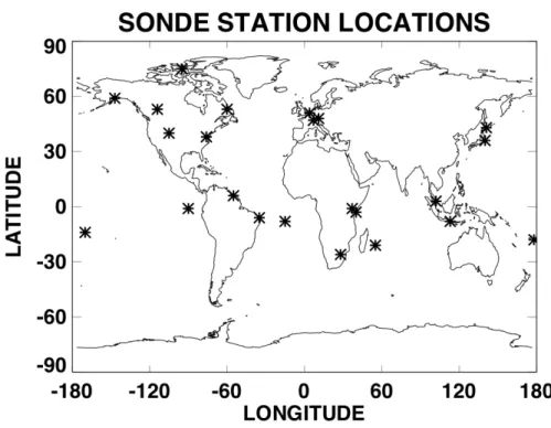
(Thompson et al., 2003a), which started in 1998; two of these are in the northern hemi-sphere (NH). We use data from 12 extratropical stations in the NH. Station details are given in Table 1 and shown in Fig. 1.
The analysis was the same as that in Logan (1999a) with the following differences:
5
the base period for the analysis was updated to 1985–2000 for the extratropical sta-tions, and to all available data for the tropical stasta-tions, which have shorter records; the pressure levels were changed from irregular intervals (1000, 900, 800 hPa etc.) to 35 levels equally spaced in pressure altitude between 1000 and 5 hPa (∼1 km apart), and averages were formed for each pressure level, with interpolation used only if there
10
were no measurements in a layer. This last change was made because the data are now available with much higher vertical resolution than previously, when the poor res-olution required that interpolation be used.
Exactly the same profiles were used to form the monthly means on the pressure levels and on the altitude grid relative to the thermal tropopause. Some profiles were
15
eliminated from the analysis as the tropopause levels derived from the temperature profiles were clearly unrealistic, as discussed in Logan (1999a). The data relative to the tropopause were interpolated to a grid with 1 km resolution in geometric altitude, extending from 6 km below the tropopause to 12 km above it. These profiles were averaged together to produce monthly means relative to the tropopause, the RTT
cli-20
matology. There are about 150 profiles in the monthly means for the European sonde stations, about 80 for the other extratropical stations, and about 22 for the tropical stations.
Several factors motivated the choice to use the thermal tropopause as a refer-ence. Temperature is simultaneously measured with ozone for each sonde,
provid-25
ing a straightforward and high-resolution profile enabling accurate identification of the thermal tropopause. Use of a dynamical tropopause definition based on potential vor-ticity (PV) would require interpolating relatively low vertical and horizontal resolution PV fields from one of several available analyzed data sets to the sonde profiles. Pan et
ACPD
8, 1589–1634, 2008 Evaluation of GMI Combo model near-tropopause ozone D. Considine et al. Title Page Abstract Introduction Conclusions References Tables Figures ◭ ◮ ◭ ◮ Back Close Full Screen / EscPrinter-friendly Version Interactive Discussion al. (2004) found that the chemical transition layer surrounding the tropopause defined
by CO and O3 correlations centered on the thermal tropopause, also supporting the use of the thermal tropopause.
3 Model and run description
The GMI Combo model is described in Duncan et al. (2007) and Strahan et al. (2007).
5
The basic structure of the Combo model, without photochemical modules, is also given in Considine et al. (2005). Here, we present details salient to this study. The Combo model is an outgrowth of the original GMI model, a stratospheric CTM described in Rotman et al. (2001). The complete Combo model also includes a full treatment of both stratospheric and tropospheric photochemistry. In this study, we run the Combo model
10
at horizontal resolutions of 4◦latitude by 5◦longitude and 2◦by 2.5◦. The model has 42
levels, extending from the surface up to 0.01 hPa. The resolution at the tropopause is about 1 km.
For this study, the Combo model was driven by meteorological data generated from a 50-year run of the GMAO GEOS4 AGCM (Bloom et al., 2005). This run was driven
15
by observed sea surface temperatures, but was otherwise unconstrained. We use a 5-year subset corresponding to the years 1994–1998. The GEOS4 AGCM has both deep (Zhang and McFarlane, 1995) and shallow (Hack, 1994) convective transport parameterizations.
The Combo model uses a 114-species chemical mechanism combining the
strato-20
spheric mechanism of Douglass et al. (2004) with the tropospheric chemical mecha-nism of Bey et al. (2001). Species transport is calculated using the flux-form semi-Lagrangian scheme of Lin and Rood (1996). The chemical mechanism describes both stratospheric halogen chemistry and tropospheric nonmethane hydrocarbon chemistry, including isoprene oxidation. Both stratospheric and tropospheric heterogeneous
re-25
actions are included in the chemical mechanism. PSCs are parameterized using the scheme of Considine et al. (2000). Tropospheric heterogeneous reactions occur on
ACPD
8, 1589–1634, 2008 Evaluation of GMI Combo model near-tropopause ozone D. Considine et al. Title Page Abstract Introduction Conclusions References Tables Figures ◭ ◮ ◭ ◮ Back Close Full Screen / EscPrinter-friendly Version Interactive Discussion tropospheric sulfate, dust, sea-salt, and organic and black carbon aerosol distributions
generated by the Goddard Chemistry, Aerosol, Radiation and Transport model (Chin et al., 2002).
Mixing ratio boundary conditions for stratospheric source gases, N2O, and CH4
cor-respond to the mid-1990’s. Surface emission inventories are described in Bey et
5
al. (2001) and Duncan et al. (2003), and represent rates typical of the mid-1990’s. Lightning NOxis also included as monthly mean emissions fields. The lightning source
is 5.0 Tg N/y. The horizontal distribution of lightning emissions is based on the ISCCP deep convective cloud climatology as described in Price et al. (1997). Lightning flash rates are from Price and Rind (1992), and the vertical distribution of lightning NOx is
10
based on the cloud resolved convection simulations of Pickering (1998).
The initial condition was taken from a 10-year spinup run of the Combo model, which is enough time for stratospheric species to converge to an approximate annually repeat-ing steady-state condition well above the lower stratosphere, the focus of this study. Diurnal average 3-D gridded ozone distributions were output daily. These were
inter-15
polated to the ozonesonde station locations, and used to construct the monthly average profiles we compare to observations in the next section.
4 Results
4.1 Global comparisons
We first provide a global-scale perspective for subsequent comparisons with the
20
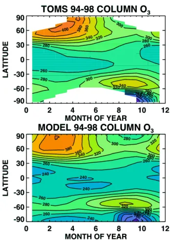
ozonesonde climatologies. Figure 2 compares model column ozone distributions from the 2◦
×2.5◦model run throughout the year with 1994–1998 average column ozone from the merged Total Ozone Mapping Spectrometer (TOMS)/Solar Backscatter Ultraviolet (SBUV) measurement data set (Stolarski and Frith, 2006). The model reproduces well the observed average global total ozone distribution during this time period. The
an-25
nual cycle of tropical total ozone is represented well, though model values are about 1595
ACPD
8, 1589–1634, 2008 Evaluation of GMI Combo model near-tropopause ozone D. Considine et al. Title Page Abstract Introduction Conclusions References Tables Figures ◭ ◮ ◭ ◮ Back Close Full Screen / EscPrinter-friendly Version Interactive Discussion 20 DU low compared to the TOMS observations. The model NH springtime peak of
∼400 DU is a few DU low, occurs ∼2 weeks early, and is not distinctly off the pole as is the case with the observations. The NH high latitude summertime ozone decrease is reproduced well. In the SH, the model area over 340 DU is smaller than observed, but is otherwise in good agreement. The model produces a convincing ozone hole. Low
5
model values at high latitudes during the SH summer suggest a somewhat too-isolated SH polar region during the spring and summer. Since total ozone is very sensitive to the stratospheric residual circulation, the good agreement between observed and modeled total ozone suggests that the stratospheric residual circulation of the GEOS-4 AGCM is fairly realistic.
10
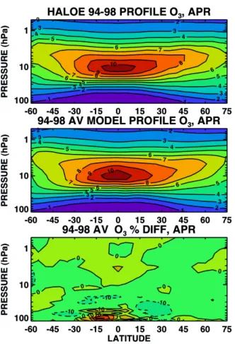
Figure 3 compares the model zonal mean distribution of stratospheric ozone in April from the 2◦×2.5◦ model run with observations made during April by the Halogen Oc-cultation Experiment (HALOE) on board the Upper Atmosphere Research Satellite (UARS) between 1994 and 1998 (Russell et al., 1993). The figure shows excellent cor-respondence between the observations and the model throughout most of the
strato-15
sphere. The model is generally within 10% of observations. There is a high-bias of up to 30% in the tropical lower stratosphere compared to HALOE observations, which will be discussed further below. Overall, the comparison reveals no serious deficiencies in the model representation of stratospheric ozone distributions.
The 4◦
×5◦ model run also compares very well with the merged total ozone and
20
HALOE data (not shown). The differences that exist, such as a shallower ozone hole and somewhat larger model high-biases in the tropical lower stratosphere, are gener-ally minor in this global perspective.
4.2 Tropopause heights
As a test of model meteorological characteristics in the NTR, we first compare modeled
25
and observed tropopause heights at selected stations in Fig. 4. Solid lines show mean values, dashed lines show medians. The stations were chosen to span the latitude range of the observations and show typical results. The differences between monthly
ACPD
8, 1589–1634, 2008 Evaluation of GMI Combo model near-tropopause ozone D. Considine et al. Title Page Abstract Introduction Conclusions References Tables Figures ◭ ◮ ◭ ◮ Back Close Full Screen / EscPrinter-friendly Version Interactive Discussion mean and median tropopause heights are small at all stations in both the observations
and the model. There is good agreement between modeled and observed tropopause pressures, including the annual cycle. Differences are largest at Resolute (75◦N) and at Wallops Island (38◦N).
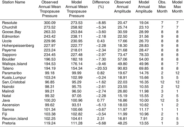
Table 2 provides a summary of the comparisons for all stations. The model
5
tropopause is typically at slightly lower pressures than observed, except for Uccle, Paramaribo, Java, and Reunion Island. There is anomalously poor agreement at Tateno (36◦N), with model pressures ∼21% lower than observations. This is
primar-ily a consequence of temperature profiles with double tropopauses, which sometimes occur near the subtropical jet. Due to this poor agreement, we exclude Tateno from
10
further analysis.
4.3 Tropopause ozone
Figure 5 compares for the 4◦×5◦model run the annual cycle of observed monthly mean tropopause ozone (black line) with model monthly mean tropopause ozone (red line) and model ozone values sampled at observed tropopause altitudes (blue line). Ozone
15
at the model tropopause is higher than observed values, both in the tropics and NH extratropics and throughout the year. Figure 5 shows that the model high bias is oc-casionally due simply to a higher tropopause in the model than observations – for instance, at Resolute after March. However, at most other locations model ozone is high-biased even at the observed tropopause. Figure 5 also shows that the annual
cy-20
cle of model tropopause ozone is generally similar in phasing to the observations. The absolute magnitude of the annual cycle in the model at these locations is also similar to the observations, though in percentage terms the annual cycles are somewhat weaker than is observed.
Figure 6 shows results for the 2◦×2.5◦ run. The tropopause ozone bias in the
extrat-25
ropics is largest during the spring and summer. At Resolute, Goose Bay, and Edmon-ton, peak ozone values are about 75 ppbv higher than the 4◦×5◦ run. At Payerne and Sapporo, there are smaller increases of ∼30 ppbv. The tropical stations show a smaller
ACPD
8, 1589–1634, 2008 Evaluation of GMI Combo model near-tropopause ozone D. Considine et al. Title Page Abstract Introduction Conclusions References Tables Figures ◭ ◮ ◭ ◮ Back Close Full Screen / EscPrinter-friendly Version Interactive Discussion ozone high bias compared to the 4◦
×5◦run.
Figure 7 shows the percent difference between modeled and observed annually av-eraged tropopause ozone for all stations, as a function of station latitude. Results for both the 4◦
×5◦ and 2◦×2.5◦ model runs are shown. In the extratropics (38◦–75◦N), where annual mean tropopause ozone is 116–149 ppbv, the model has a high bias of
5
36–72% in the 4◦×5◦run (mean 45%). The extratropical high bias in the 2◦×2.5◦model run is significantly larger, with the mean bias increasing to ∼61%. However, there are reductions for Boulder and Wallops Island, the two lowest-latitude midlatitude stations considered. In the tropics, observed annual mean tropopause ozone is 58–130 ppbv. The 4◦
×5◦ run shows a high bias of 17–63% (mean 43%) in the tropics. This drops to
10
∼31% in the 2◦×2.5◦ model run.
The fact that model tropopause high biases are larger in the 2◦×2.5◦ run at midlati-tude stations, and smaller in the tropics, may be explained by lower effective horizontal diffusion in the higher resolution run. Strahan and Polansky (2006) showed that simula-tions at 2◦×2.5◦better resolved the stratospheric subtropical and polar mixing barriers,
15
leading to larger horizontal gradients and improving the simulation of stratospheric dy-namical features. Reduced horizontal mixing between the tropics and the midlatitudes would tend to decrease tropical mixing ratios and increase those at mid and higher latitudes.
A possible explanation for the ozone high bias at the tropopause seen in both
sim-20
ulations is an overly vigorous residual circulation in the GEOS 4 AGCM. Strahan et al. (2007) found overly strong ascent and mixing in the GEOS 4 AGCM tropical lower stratosphere, particularly during the fall, suggesting that the residual circulation may be too strong. Since according to Olsen et al. (2007) the residual circulation is strongly correlated with stratosphere-troposphere exchange, we performed linear regressions
25
of the 60 (5 years at 12 months/year) zonal mean, monthly mean O3 values at each
NH latitude and pressure level in the 4◦×5◦run of the Combo model with the 60 values of monthly mean NH extratropical cross-tropopause O3 flux, calculated as described in Olsen et al. (2004). From these regressions we calculated at each latitude and
ACPD
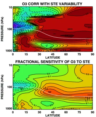
8, 1589–1634, 2008 Evaluation of GMI Combo model near-tropopause ozone D. Considine et al. Title Page Abstract Introduction Conclusions References Tables Figures ◭ ◮ ◭ ◮ Back Close Full Screen / EscPrinter-friendly Version Interactive Discussion pressure level the linear correlation and fractional sensitivity (percent change in O3per
percent change in flux) of zonal mean, monthly mean O3 with the monthly mean NH
cross-tropopause flux of O3. This is shown in Fig. 8. The top panel of Fig. 8 shows that
O3 near the tropopause is strongly positively correlated with STE poleward of ∼30◦. The correlation remains high throughout most of the extratropical stratosphere. The
5
bottom panel suggests that a 1% increase in STE results in an ∼0.5–0.6% increase in tropopause O3. Given the NH mean high bias of ∼45%, Fig. 8 suggests that a reduction in STE of ∼90% would be required to eliminate the model high bias at the tropopause in the NH.
Model STE of NH extratropical O3in the 4◦×5◦ run is −266±9 Tg yr−1, which agrees
10
well with several other estimates (Olsen et al., 2004). A 90% reduction is therefore un-reasonable. Changes to the residual circulation of the magnitude necessary to reduce STE by 90% would also adversely affect the good agreement of stratospheric O3with
observations shown in Figs. 2 and 3, in addition to increasing the tropical tropopause ozone high bias. Thus Fig. 8 does not support the idea that the ozone high biases at the
15
model tropopause can be explained simply by an overly vigorous residual circulation and consequently too much STE. Additional evidence for the soundness of the GEOS4 AGCM meteorological data is provided in Strahan et al. (2007), which demonstrates that transport processes connecting the tropical lower and upper troposphere, and be-tween the tropical UT and the extratropical lowermost stratosphere are represented
20
correctly.
Other possible contributors to the model high bias include insufficient vertical reso-lution at the tropopause and an overly vertically diffusive transport scheme. Rasch et al. (2006) demonstrated that the Lin and Rood transport scheme used in the Combo model is substantially less vertically diffusive than other popular schemes for
simulat-25
ing tracer transport in the NTR. Thus it is most likely that higher vertical resolution in the NTR is necessary to eliminate the high bias of tropopause ozone.
ACPD
8, 1589–1634, 2008 Evaluation of GMI Combo model near-tropopause ozone D. Considine et al. Title Page Abstract Introduction Conclusions References Tables Figures ◭ ◮ ◭ ◮ Back Close Full Screen / EscPrinter-friendly Version Interactive Discussion 4.4 Effects of averaging method on ozone gradients
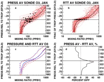
In making comparisons of the observed and modeled vertical distribution of ozone, we consider two approaches: a pressure coordinate and a vertical coordinate defined relative to the tropopause. We illustrate the differences between the two averaging methods in Fig. 9. Figure 9a shows as a function of pressure the 49 sonde profiles
5
in the climatologies sampled at Edmonton for Januarys between 1985 and 2000 (red lines), the monthly average vertical profile averaged at constant pressure levels, and one standard deviation error profiles (black lines). The figure shows that tropopause pressures (black crosses) are spread over the region within about one half of an e-fold of the monthly median tropopause pressure. Figure 9b shows the same profiles in a
10
RTT coordinate system, as well as the monthly mean profile averaged in RTT coordi-nates along with the plus and minus standard deviations. It is obvious that the profiles are more organized in Fig. 9b compared to Fig. 9a, especially near the tropopause, be-cause a substantial fraction of the variability is related to daily changes in tropopause height. Fig. 9c compares the monthly average profiles and the standard deviations
15
shown in Fig. 9a and b. It is important to note that to plot the RTT-average profile as a function of pressure in Fig. 9c, we have normalized the RTT-average profile relative to the monthly median tropopause pressure. Figure 9c illustrates that pressure-averaging results in weaker cross-tropopause gradients and larger UT ozone mixing ratios than the RTT-averaged values near the tropopause. RTT-averaging also reduces the
vari-20
ability near the tropopause. Figure 9d shows the percent deviation of the pressure-averaged profile from the RTT-pressure-averaged profile. Differences peak in the UT, with pres-sure averaged values up to 40% higher than RTT-averaged results.
Figure 10 shows model ozone profiles at Edmonton. (Results from the 2◦×2.5◦run are shown, but there is little difference between the two resolutions.) Figure 10a shows
25
that model tropopause pressure variablity is similar to observations (the standard devi-ation of the model tropopause pressure at Edmonton during January is ∼20% smaller than observations). As is observed, the RTT-averaged profiles shown in Fig. 10b are
ACPD
8, 1589–1634, 2008 Evaluation of GMI Combo model near-tropopause ozone D. Considine et al. Title Page Abstract Introduction Conclusions References Tables Figures ◭ ◮ ◭ ◮ Back Close Full Screen / EscPrinter-friendly Version Interactive Discussion more organized than in Fig. 10a. Unlike the observations, Fig. 10c shows similar
but smaller differences between pressure averaging and RTT-averaging, both in the change in upper tropospheric ozone values and profile variability. Figure 10d shows that the percent deviation of the pressure-averaged profile from the RTT-averaged pro-file is ∼8%, smaller than the observed ∼40% difference shown in Fig. 9d.
5
The results shown in Figs. 9d and 10d are typical at other locations and times of year. Model discrepancies between the two averaging techniques are generally small, while the differences between observed profiles averaged using these two techniques are much larger. Logan (1999a) showed that the vertical gradient in monthly averaged ozone profiles constructed from sondes is on the order of a factor of 2 steeper when
10
averaged relative to the tropopause. Here, we see that the model does not correctly reproduce the atmosphere in this regard. As a result, good agreement between mod-eled and observed pressure-averaged results does not imply good correspondence between modeled and observed cross-tropopause O3 profiles. Comparing RTT aver-ages should provide a more accurate picture of the discrepancies between the model
15
and observations.
We suggest an explanation of the model insensitivity to averaging technique, with the following heuristic example: Presume that the ozone change in the model between its characteristic stratospheric and tropospheric values is given by ∆O3, and the
char-acteristic vertical depth of the region over which the transition occurs is given by the
20
distance ∆zNTR. Then the ozone gradient across this region in a daily ozone profile is
justS=∆O3/∆zNTR. Over the course of a month, the transition region will move up and
down in altitude as the tropopause height varies by some amount ∆zTROP. The RTT
average will be insensitive to this movement, so we will just have: <S>RTT∼S.
How-ever, the tropopause variability will smear the gradient in a pressure average, giving a
25
slope of: <S>PRESS∼∆O3/(∆zNTR+∆zTROP)=<S>RTT×∆zNTR/(∆zNTR+∆zTROP). This
equation suggests that the larger the size of the transition region between the tropo-sphere and stratotropo-sphere (∆zNTR) relative to the monthly variability of the tropopause
height (∆zTROP), the smaller the difference between RTT and pressure averaging. Thus
ACPD
8, 1589–1634, 2008 Evaluation of GMI Combo model near-tropopause ozone D. Considine et al. Title Page Abstract Introduction Conclusions References Tables Figures ◭ ◮ ◭ ◮ Back Close Full Screen / EscPrinter-friendly Version Interactive Discussion the weakness of the daily profile vertical gradients shown in Fig. 10b can produce a
smaller than observed sensitivity to the averaging technique. The equation also sug-gests that overly weak tropopause pressure variability can result in low sensitivity to averaging technique. However, the ∼20% weaker tropopause height variability seen in the model is not large enough to account for the much weaker model sensitivity to
5
averaging technique compared to observations. 4.5 Profile ozone comparisons
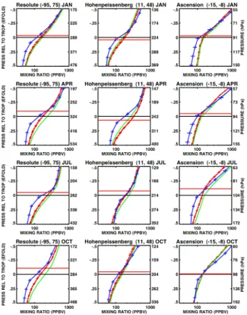
Figure 11 shows 2◦×2.5◦ run profile comparisons with observations of ozone mix-ing ratios from a pressure of half an efold below the observed monthly median tropopause pressure to half an efold above at Resolute, Hohenpeissenberg, and
As-10
cension. Shown are model RTT-averaged monthly mean profiles, plotted relative to the model monthly median tropopause (red), and relative to the observed monthly me-dian tropopause (green). Plotting relative to the observed monthly meme-dian tropopause allows comparison of modeled and measured RTT-averaged profiles at the same frac-tion of the tropopause pressure. (For instance, wheny=.25, the observed profiles and
15
the model profile represented by the green line are a factor ofe0.25 higher than their respective tropopause pressures.)
The RTT-averaged model profiles shown in Fig. 11 reproduce the characteristic shapes seen in the observations, but typically with weaker cross-tropopause gradi-ents resulting in model high biases in the UT and sometimes low biases above the
20
tropopause. Model profiles can reproduce the observations quite well, such as at Ho-henpeissenberg in July, but often the upper tropopause high bias is substantial. It is interesting to note that normalizing the model profiles to the observed rather than mod-eled monthly median tropopause tends to increase the upper-tropopause high bias when the model tropopause lies above (at a lower pressure, which is typical) the
ob-25
served monthly median tropopause, and decrease it when the model tropopause is found below the observed tropopause. This effect is distinct from RTT-averaging pro-cess itself. While it is obvious that RTT averaging produces comparisons that better
ACPD
8, 1589–1634, 2008 Evaluation of GMI Combo model near-tropopause ozone D. Considine et al. Title Page Abstract Introduction Conclusions References Tables Figures ◭ ◮ ◭ ◮ Back Close Full Screen / EscPrinter-friendly Version Interactive Discussion characterize model/measurement disfferences across the tropopause than pressure
averaging, it is not clear if it is better to compare model and observed profiles at the same pressure or at the same fraction of their respective tropopause pressures.
Figure 12 shows percent differences between the model and observed monthly mean profiles for the three stations shown in Fig. 11. (Note the larger vertical range in
5
Fig. 12.) Here we show percent differences between model and observed pressure-averaged profiles (red), RTT-pressure-averaged profiles (blue), and RTT-pressure-averaged profiles nor-malized relative to the observed tropopause (green). Figure 12 shows better agree-ment between the modeled and observed pressure-averaged monthly mean ozone profiles than the RTT-averaged profiles, as expected. The pressure-averaged profiles
10
show moderate model high-biases in the UT by ∼20–50%. The bias in the lower strato-sphere is smaller in magnitude and more variable between a high or low bias than in the UT. When RTT-averaging is used, biases between the model and the observations are larger; differences are typically about ∼50%, but can exceed 100% (blue lines). When RTT-averaged profiles are compared at the same fractional value of the tropopause
15
pressure (green lines), the model upper tropospheric high bias tends to be increased when the model tropopause pressure is lower than the observed tropopause pressure, as was also shown in Fig. 11.
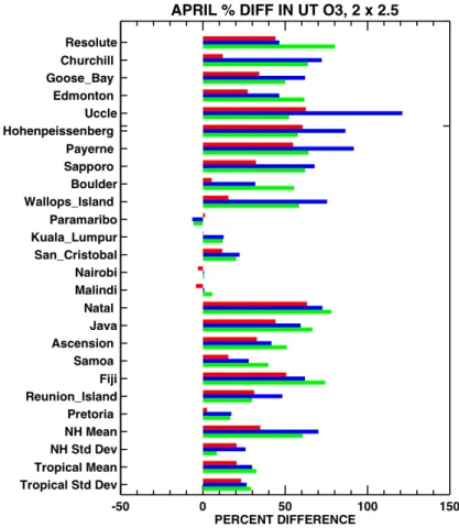
Figure 13 is a bar chart summarizing April percent differences between the 2◦×2.5◦ model run and observed ozone in the UT, at a pressure one quarter of an e-fold higher
20
than the tropopause pressure. April is shown because the largest UT model discrep-ancies from observations occur in the March/April time period, while the smallest occur in June and July. Figure 13 illustrates that RTT-averaged (blue bars) and RTT-averaged profiles normalized to the observed tropopause (green bars) typically show substan-tially larger biases than the pressure-averaged profiles (red bars) at both the tropical
25
and NH stations. The tropical stations of Paramaribo, Kuala Lumpur, San Cristobal, Nairobi, and Malindi exhibit particularly small biases. The mean NH pressure-averaged bias is ∼35%, which approximately doubles with RTT-averaging. In the tropical mean, there are ∼20% high biases in the pressure-averaged case vs. a ∼30% difference for
ACPD
8, 1589–1634, 2008 Evaluation of GMI Combo model near-tropopause ozone D. Considine et al. Title Page Abstract Introduction Conclusions References Tables Figures ◭ ◮ ◭ ◮ Back Close Full Screen / EscPrinter-friendly Version Interactive Discussion RTT-averaged profiles, resulting in a ∼50% difference between the averaging
tech-niques.
Figure 14 shows the biases at all stations in the lower stratosphere, at a pressure one quarter of an e-fold below the observed monthly median tropopause pressure. Agreement in the lower stratosphere is generally substantially better than in the
up-5
per troposphere, with mean biases in the NH and the tropics<20%. Here, the RTT-averaged and normalized RTT-RTT-averaged biases are typically more negative than the biases between pressure-averaged profiles. This is the expected behavior of a pro-file with a weak cross-tropopause gradient – high biases in the UT, and low biases in the lower stratosphere. The five tropical stations with small UT high biases are shown
10
here to have more substantial low biases in the lower stratosphere, indicating that the agreement of model cross-tropopause gradients with observations at these stations is similar to other stations.
Compared to the 4◦
×5◦run, the 2◦×2.5◦ run shows poorer agreement with observa-tions at higher midlatitudes than the 4◦×5◦run, and similar agreement in the lower
mid-15
latitudes and tropics. Thus, increasing horizontal model resolution does not generally improve agreement between the ozonesonde observations and the model simulations in the NTR. The 2◦×2.5◦run high-bias increases at high-latitude stations suggests that the better-defined stratospheric subtropical and polar mixing barriers in the 2◦×2.5◦run may have increased STE at higher latitudes, resulting in larger ozone concentrations
20
at higher midlatitudes in the NTR. 4.6 Ozone annual cycle
We now evaluate the model’s ability to reproduce observed variations in phasing and amplitude of the annual cycle of O3 as a function of pressure. As noted by Logan (1999a, b) and references therein, the peak in the observed midlatitude ozone
an-25
nual cycle occurs in the late winter/early spring in the lower stratosophere and is the result of stratospheric dynamical processes. In the midlatitude mid-troposphere, the peak occurs in the late spring/early summer and is influenced by tropospheric
ACPD
8, 1589–1634, 2008 Evaluation of GMI Combo model near-tropopause ozone D. Considine et al. Title Page Abstract Introduction Conclusions References Tables Figures ◭ ◮ ◭ ◮ Back Close Full Screen / EscPrinter-friendly Version Interactive Discussion cal processes as well as stratospheric input. Vertical changes in phasing and amplitude
therefore test the model coupling between the stratosphere and troposphere.
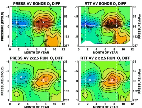
Figure 15 compares the percent deviation from the annual mean of the modeled and observed annual cycle of tropical ozone as a function of pressure. The figure shows the average over deep tropical stations within 10◦ of the equator. While there
5
is some variability amongst the tropical stations (Thompson et al., 2003b), an average over these stations is reasonably representative. The top left and right panels of Fig. 15 show pressure-averaged and averaged results, respectively. To construct the RTT-averaged annual cycles, the monthly RTT-RTT-averaged profiles were first interpolated to pressure coordinates using monthly median tropopause pressures. The bottom left
10
and right panels show model pressure- and RTT- averaged results for the 2◦
×2.5◦run, respectively. Figure 15 shows that the strongest annual cycle is observed at or just above the tropopause. In the observed RTT-averaged case (top right), the extrema have a greater magnitude, are temporally broader and vertically narrower compared to the pressure-averaged case.
15
The vertical variation of the amplitude and phasing of the model tropical annual cycle shown in Fig. 15 is qualitatively quite similar to the observations. However, the largest peak-to-peak amplitudes of the model annual cycles (∼43% and ∼51% for the pres-sure and RTT-averaged runs, respectively) just above the tropopause are weaker than the observed ∼70% and ∼88% variation in the pressure-averaged and RTT-averaged
20
climatology, respectively.
Randel et al. (2007) present an analysis of the annual cycle in the vertical profile of tropical ozone, which argues that the fractional amplitude (i.e., amplitude divided by annual average) of the annual cycle in O3 mixing ratio is the product of the annual cycle amplitude in residual mean upwelling in the lower stratosphere and the fractional
25
vertical gradient of annually averaged O3 in the tropics; the largest amplitude occurs
where the O3fractional vertical gradient is the largest. If this also holds for the model, its agreement with observations will depend on how well the model reproduces observed annual cycles in upwelling and annually averaged O3fractional vertical gradients.
ACPD
8, 1589–1634, 2008 Evaluation of GMI Combo model near-tropopause ozone D. Considine et al. Title Page Abstract Introduction Conclusions References Tables Figures ◭ ◮ ◭ ◮ Back Close Full Screen / EscPrinter-friendly Version Interactive Discussion Figure 16 compares the observed and modeled fractional vertical gradients in
trop-ical, annually averaged O3 mixing ratio. The figure shows that the fractional verti-cal gradients are largest just above the tropopause for both the observations and the model runs. The observed fractional vertical gradients in the RTT-averaged case are substantially larger than the pressure-averaged case, with peak vertical gradients of
5
∼97%/km and ∼67%/km, respectively. Neither the 4◦×5◦ or the 2◦×2.5◦ model runs show much difference between pressure – and RTT-averages. The model fractional vertical gradients peak at ∼58–59% km in both runs, ∼11% less than the observed pressure-averaged case. According to the Randel et al. (2007) analysis, this should result in an annual amplitude ∼11% lower than observed provided the modeled and
10
observed vertical upwelling is equivalent. As shown in Fig. 15, the model pressure-averaged amplitude of 43% is ∼39% lower than observations. According to the Randel et al. (2007) analysis, this low bias indicates that in the model, the amplitude of the annual cycle in vertical upwelling at the tropopause level is ∼30% weaker than in the real atmosphere.
15
It is worth pointing out that the amplitude of the O3 annual cycle in the 4◦×5◦ model
run is larger than in the 2◦
×2.5◦ run, with largest peak-to-peak amplitudes of 49% and 59%, in the pressure-averaged and RTT-averaged cases, respectively. The 49% amplitude is ∼30% lower than observations and suggests an upwelling ∼20% weaker than observations. However, resolution changes should not affect vertical upwelling,
20
and Figure 16 shows that the vertical O3gradients are not resolution-dependent. The
differences between the two resolutions may thus be due to some influence in the model of horizontal transport on the tropical seasonal cycle of O3.
Figure 15 shows that the annual maximum at pressures about half an e-fold below the tropopause occurs in October/November. The peak here is unlikely to be related to
25
the annual cycle near the tropopause, because vertical ozone gradients are relatively low at these pressures, as indicated by Fig. 16. The signal is observable at most of the tropical sites, but is particularly strong at Fiji, Natal, and Reunion Island. The amplitude in the model is about half of the observed peak values. The model/measurement
ACPD
8, 1589–1634, 2008 Evaluation of GMI Combo model near-tropopause ozone D. Considine et al. Title Page Abstract Introduction Conclusions References Tables Figures ◭ ◮ ◭ ◮ Back Close Full Screen / EscPrinter-friendly Version Interactive Discussion discrepancy is particularly large at Natal. It is well-known that biomass burning plays a
strong role in tropical ozone during September–October (Thompson, 1996; Galanter et al., 2000), with lightning providing an important source of NOx at the beginning of the
wet season (Martin et al., 2000). Although biomass burning emissions are included in the model, it may be that the Combo model underestimates its impact on tropical O3
5
concentrations in the mid-troposphere.
Figure 17 compares modeled and observed annual cycles at midlatitudes, following Fig. 15. (Resolute was excluded due to its high latitude.) The observed pressure-averaged and RTT-pressure-averaged plots are very similar. Both show the maximum in the annual cycle occurring in March or April, one to two months after the annual tropopause
10
pressure minimum. The minimum of the annual cycle occurs in both cases one month after the occurrence of the annual tropopause maximum. Peak to peak amplitude of the annual cycle is ∼90%. The RTT-average plot shows a closer association of the ozone annual cycle at the tropopause level with the annual cycle in tropopause height, as the peak occurs above the tropopause and the minimum occurs below the tropopause.
15
Both panels show a phase shift in the timing of the peak above the tropopause to earlier in the year at higher altitudes. Below the tropopause the two panels both display the well-known shift in the phase of the peak from March/April to June/July in the mid-troposphere. However, in the RTT-average climatology shown in the middle panel, this shift is clearer.
20
The bottom panel of Fig. 17 shows the midlatitude annual cycle from the 2◦
×2.5◦ run. The 4◦×5◦ run annual cycle is very similar. The model reproduces the observed changes in phase and amplitude of the annual cycle in ozone very well, with a peak-to-peak amplitude of ∼90% at the pressure level of the tropopause that is only slightly weaker than observations. There is less of a phase shift at higher pressures in the
25
stratosphere, and the March/April peak amplitude shift to later in the year below the tropopause is less pronounced. Overall, however, the midlatitude agreement of the model with the observations is better than at tropical stations.
ACPD
8, 1589–1634, 2008 Evaluation of GMI Combo model near-tropopause ozone D. Considine et al. Title Page Abstract Introduction Conclusions References Tables Figures ◭ ◮ ◭ ◮ Back Close Full Screen / EscPrinter-friendly Version Interactive Discussion
5 Summary and conclusion
The GMI Combo model fully resolves the important processes in the troposphere and stratosphere, uses a transport scheme shown to represent well vertical gradients in the NTR, and has been integrated using a modern GCM-based meteorological data set to minimize the possible effects of anomalous vertical diffusion that affects analyzed
me-5
teorological data. We have examined the ability of the Combo model to represent O3 distributions in the NTR by comparing it to two climatological O3data sets constructed
from ozonesondes. The ozonesonde observations have the high vertical resolution necessary for tropopause-level evaluations. They have been averaged both on pres-sure surfaces and relative to the tropopause, and include a relatively large amount of
10
tropical data. We have tested the sensitivity of the results to horizontal resolution by considering both 4◦×5◦and 2◦×2.5◦ versions of the model.
The overall stratospheric distribution of ozone produced by the GMI Combo model is in good agreement with satellite observations, suggesting the meteorological data represents the stratospheric residual circulation well. Despite this good agreement,
15
Combo model annual mean ozone distributions are biased high at the 4◦
×5◦ model thermal tropopause, by ∼45% in both the SH tropics and NH midlatitudes. When model resolution is increased, the high bias increases to ∼61% in the NH midlatitudes and decreases to ∼31% in the tropics. Such an effect is expected due to a decrease in effective horizontal diffusivity in the higher resolution runs. We argue that problems
20
with the GEOS-4 AGCM meteorology cannot explain the high biases because of the good agreement of our global ozone comparisons with observations, the unrealistically large changes in residual circulation we estimate are necessary to remove the bias, and the results of the Strahan et al. (2007) tests of the transport processes in the GEOS 4 AGCM. We then infer that insufficient vertical resolution near the tropopause and/or
25
too high vertical diffusivity are the likely causes. In a similar study, Pan et al. (2007) also find vertical resolution and diffusivity important to simulations of near-tropopause ozone distributions.
ACPD
8, 1589–1634, 2008 Evaluation of GMI Combo model near-tropopause ozone D. Considine et al. Title Page Abstract Introduction Conclusions References Tables Figures ◭ ◮ ◭ ◮ Back Close Full Screen / EscPrinter-friendly Version Interactive Discussion The tropopause O3high biases in the Combo model would produce erroneous
esti-mates of extratropical ozone STE if the method of calculation used tropopause ozone mixing ratios to calculate STE. The differential method for inferring STE presented in Olsen et al. (2004) is insensitive to tropopause ozone values, because it uses the balance between the changing amount of ozone in the lowermost stratosphere and
5
ozone flux into the lowermost stratosphere to calcuate ozone crossing the tropopause. However, Olsen et al. (2004) do use tropopause ozone mixing ratios to calculate the relative amounts of diabatic and adiabatic STE. The use of the GMI Combo model in such a calculation would result in an overestimate of diabatic and an underestimate of adiabatic ozone STE.
10
The method of averaging observations and data to produce monthly mean profiles for comparison is an important consideration for UT comparisons. RTT-averaging reveals more significant model/measurement discrepancies in the UT than does pressure-averaging in both the SH tropics and NH midlatitudes. NH mean UT high O3 high biases during April in the model increase from ∼35%±20% to ∼70%±10% when
pro-15
files are RTT-averaged. The effect in the tropics is smaller, with ∼20%±25% biases increasing to ∼30%±28% with RTT averaging. This occurs because RTT-averaging of the ozonesondes better preserves the strong vertical gradients characterizing daily ozonesonde profiles than does pressure averaging. The RTT-comparisons show that the model tends to underestimate the sometimes abrupt transition between the
tropo-20
sphere and the stratosphere seen in individual ozonesondes. Increasing the horizontal resolution of the model does not change this result much. Increasing the vertical reso-lution of the model (including the resoreso-lution of the meteorology) may produce stronger vertical ozone gradients in individual profiles and consequently better agreement with observations.
25
In the lower stratosphere, modeled and observed O3 concentrations agree very well regardless of averaging technique. NH mean lower stratospheric biases are ∼10%±10%, for both pressure and RTT-averaged cases. In the tropics, the mean biases are ∼10%±10% for pressure averaging, or ∼−20%±10% for RTT-averaged
ACPD
8, 1589–1634, 2008 Evaluation of GMI Combo model near-tropopause ozone D. Considine et al. Title Page Abstract Introduction Conclusions References Tables Figures ◭ ◮ ◭ ◮ Back Close Full Screen / EscPrinter-friendly Version Interactive Discussion sults. Strahan et al. (2007) compared Combo model ozone distributions to Aura MLS
observations in the tropics and extratropics at potential temperatures between 350– 400 K, which are generally above the tropopause level. They also found very good agreement with MLS ozone during all seasons in the extratropics. This is consistent with our results that the model high bias tends to occur at and below the tropopause
5
level. Strahan et al. (2007) also found the model to be low-biased relative to version 1.5 Aura MLS observations in the tropics at 350 K, but found that may be due to MLS high-biases in the tropics at 215 hPa. Since we find mean model 20–30% high biases in the tropical UT compared to sonde observations, with the bias at some tropical sta-tions reaching ∼70%, it appears that Aura MLS version 1.5 ozone in the tropical UT is
10
high-biased with respect to the sonde observations.
Observed and modeled RTT-averaged profiles can be compared either in a pressure coordinate system by normalizing to observed and model median tropopause pres-sures, or in a tropopause-relative coordinate system. When modeled and observed tropopause heights differ substantially, the two methods can produce quite different
re-15
sults that are unrelated to the averaging process itself. It is important to be aware of these differences in order to fully understand what the model/measurement compar-isons reveal.
The GMI Combo model captures the phasing but underestimates the amplitude of the observed relative annual cycle of ozone and its variation with altitude in the SH
20
tropical NTR. Following the methodology of Randel et al. (2007), the underestimate of the amplitude appears to be too large to be explained by slightly weaker than observed vertical gradients in annually averaged O3, and suggests that the annual amplitude of mean residual upwelling at the tropopause level in the model is ∼30% less than in the real atmosphere. The model reproduces well the observed relative annual cycle
25
of ozone and its variation with altitude at the NH midlatitude stations. However, the model does not have as rapid a shift from a springtime peak at the tropopause level to a summer peak in the mid-troposphere. Increases in horizontal resolution from 4◦×5◦ to 2◦
×2.5◦do not change this result, suggesting increases in vertical resolution may be 1610
ACPD
8, 1589–1634, 2008 Evaluation of GMI Combo model near-tropopause ozone D. Considine et al. Title Page Abstract Introduction Conclusions References Tables Figures ◭ ◮ ◭ ◮ Back Close Full Screen / EscPrinter-friendly Version Interactive Discussion necessary to resolve this problem.
Acknowledgements. We would like to thank S. Strahan and B. Duncan (Goddard Earth
Sci-ences and Technology Center) and W. Randel (National Center for Atmospheric Research) for helpful discussions. We thank the GMI core modeling team as well as other members of the GMI science team for their efforts that have facilitated the research described in this paper. We
5
would also like to thank I. Megretskaia (Harvard University) for her work producing the sonde-based climatologies utilized in this paper. We are grateful for support of the NASA Modeling, Analysis, and Prediction (MAP) program. (D. Anderson, program manager).
References
Bey, I., Jacob, D. J., Yantosca, R. M., Logan, J. A., Field, B. D., Fiore, A. M., Li, Q., Liu, H.,
10
Mickley, L. J., and Schultz, M. G.: Global modeling of tropospheric chemistry with assimi-lated meteorology: Model description and evaluation, J. Geophys. Res., 106, 23 073–23 095, 2001.
Bloom, S., da Silva, A., Dee, D., Bosilovich, M., Chern, J. D., Pawson, S., Schubert, S., Sienkiewicz, M., Stajner, I., Tan, W. W., and Wu, M. L.: Technical Report Series on Global
15
Modeling and Data Assimilation, Vol. 26: Documentation and validation of the Goddard Earth Observing System (GEOS) data assimilation system – Version 4, NASA/TM – 2005 – 104606, Vol. 26, 2005.
Chin, M., Ginoux, P., Kinne, S., Torres, O., Holben, B. N., Duncan, B. N., Martin, R. V., Logan, J.A., Higurashi, A., and Nakajima, T.: Tropospheric aerosol optical thickness from the
GO-20
CART model and comparisons with satellite and sunphotometer measurements, J. Atmos. Sci., 59, 461–483, 2002.
Chipperfield, M. P.: New version of the TOMCAT/SLIMCAT off-line chemical transport model: Intercomparison of stratospheric tracer experiments, Q. J. R. Meteorol. Soc., 132, 1179– 2003, 2006.
25
Considine, D. B., Douglass, A. R., Connell, P. S., Kinnison, D. E., and Rotman, D. A.: A po-lar stratospheric cloud parameterization for the global modeling initiative three-dimensional model and its response to stratospheric aircraft, J. Geophys. Res., 105, 3955–3973, 2000. Considine, D. B., Bergmann, D. J., and Liu, H.: Sensitivity of Global Modeling Initiative
chem-istry and transport model simulations of radon-222 and lead-20 to input meteorological data,
30
ACPD
8, 1589–1634, 2008 Evaluation of GMI Combo model near-tropopause ozone D. Considine et al. Title Page Abstract Introduction Conclusions References Tables Figures ◭ ◮ ◭ ◮ Back Close Full Screen / EscPrinter-friendly Version Interactive Discussion
Atmos. Chem. Phys., 5, 3389–3406, 2005,
http://www.atmos-chem-phys.net/5/3389/2005/.
Douglass, A. R. and Kawa, S. R.: Contrast between 1992 and 1997 high-latitude spring Halo-gen Occultation Experiment observations of lower stratospheric HCl, J. Geophys. Res., 104, 18 739–18 754, 1999.
5
Douglass, A. R., Schoeberl, M. R., Rood, R. B., and Pawson, S.: Evaluation of transport in the lower tropical stratosphere in a global chemistry and transport model, J. Geophys. Res., 108, D94259, doi:10.1029/2002JD002696, 2003.
Douglass, A. R., Stolarski, R. S., Strahan, S. E., and Connell, P. S.: Radicals and reservoirs in the GMI chemistry and transport model: Comparison to measurements, J. Geophys. Res.,
10
109, D16302, doi:10.1029/2004JD004632, 2004.
Duncan, B. N., Martin, R. V., Staudt, A. C., Yevich, R., and Logan, J. A.: Interannual and seasonal variability of biomass burning emissions constrained by satellite observations, J. Geophys. Res., 108(D2), 3100, doi:10.1029/2002JD002378, 2003.
Duncan, B. N., Strahan, S. E., Yoshida, Y., Steenrod, S. D., and Liveesey, N.: Model study of
15
the cross-tropopause transport of biomass burning pollution, Atmos. Chem. Phys., 7, 3713– 3736, 2007,
http://www.atmos-chem-phys.net/7/3713/2007/.
Galanter, M., Levy, H., and Carmichael, G. R.: Impacts of biomass burning on tropospheric CO, NOx, and O3, J. Geophys. Res., 105(D5), 6633–6653, 2000.
20
Gettelman, A., Kinnison, D. E., Dunkerton, T. J., and Brasseur, G. P.: Impact of monsoon cir-culations on the upper troposphere and lower stratosphere, J. Geophys. Res., 109, D22101, doi:10.1029/2004JD004878, 2004.
Hack, J. J.: Parameterization of moist convection in the National Center for Atmospheric Re-search community climate model (CCM2), J. Geophys. Res., 99, 5551–5568, 1994.
25
Holton, J. R., Haynes, P. H., McIntyre, M. E., Douglass, A. R., Rood, R. B., and Pfister, L.: Stratosphere-Troposphere Exchange, Rev. Geophys., 33, 403–439, 1995.
Horowitz, L. W., Walters S., Mauzerall, D. L., et al.: A global simulation of tropospheric ozone and related tracers: Description and evaluation of MOZART, version 2, J. Geophys. Res., 108, 4784, doi:10.1029/2002JD002853, 2003.
30
Kinnison, D. E., Brasseur, G. P., Walters, S., et al.: Sensitivity of chemical tracers to mete-orological parameters in the MOZART-3 chemical transport model, J. Geophys. Res., 112, D20302, doi:10.1029/2006JD007879, 2007.
ACPD
8, 1589–1634, 2008 Evaluation of GMI Combo model near-tropopause ozone D. Considine et al. Title Page Abstract Introduction Conclusions References Tables Figures ◭ ◮ ◭ ◮ Back Close Full Screen / EscPrinter-friendly Version Interactive Discussion
Lacis, A. A., Wuebbles, D. J., and Logan, J. A.: Radiative forcing of climate by changes in the vertical distribution of ozone, J. Geophys. Res., 95, 9971–9981, 1990.
Lin, S. J. and Rood, R. B.: Multidimensional flux-form semi-Lagrangian transport schemes, Mon. Weather Rev., 124(9), 2046–2070, 1996.
Logan, J. A.: An analysis of ozonesonde data for the troposphere: Recommendations for
5
testing 3-D models and development of a gridded climatology for tropospheric ozone, J. Geophys. Res., 104, 16 115–16 149, 1999a.
Logan, J. A.: An analysis of ozonesonde data for the lower stratosphere: Recommendations for testing models, J. Geophys. Res., 104, 16 151–16 170, 1999b.
Martin, R. V., Jacob, D. J., Logan, J. A., Ziemke, J. M., and Washington, R.: Detection of
10
a lightning influence on tropical tropospheric ozone, Geophy. Res. Lett., 27, 1639–1642, 2000.
M ¨uller, J.-F. and Brasseur, G.: Sources of upper tropospheric HOx: A three-dimensional study, J. Geophys. Res., 104, 1705–1715, 1999.
Olsen, M. A., Schoeberl, M. R., and Douglass, A. R.: Stratosphere-troposphere exchange of
15
mass and ozone, J. Geophys. Res., 109, D24114, doi:10.1029/2004JD005186, 2004. Olsen, M. A., Schoeberl, M. R., and Nielsen, J. E.: Response of stratospheric circulation
and stratosphere-troposphere exchange to changing sea surface temperatures, J. Geophys. Res., 112, D16104, doi:10.1029/2006JD008012, 2007.
Pan, L. L., Randel, W. J., Gary, B. L., Mahoney, B. L., and Hintsa, E. J.: Definitions and
20
sharpness of the extratropical tropopause: A trace gas perspective, J. Geophys. Res., 109, D23103, doi:10.1029/2004JD004982, 2004.
Pan, L. L., Wei, J. C., Kinnison, D. E., Garcia, R. R., Wuebbles, D. J., and Brasseur, G. P.: A set of diagnostics for evaluating chemistry-climate models in the extratropical tropopause region, J. Geophys. Res., 112, D09316, doi:10:1029/2006JD007792, 2007.
25
Pickering, K. E., Wang, Y. S., Tao, W. K., Price, C., and Muller, J. F.: Vertical distributions of lightning NOx for use in regional and global chemical transport models, J. Geophys. Res., 103(D23), 31 203–31 216, 1998.
Price, C. and Rind, D.: A simple lightning parameterization for calculating global lightning dis-tributions, J. Geophys. Res., 97(D9), 9919–9933, 1992.
30
Price, C., Penner, J., and Prather, M.: NOx from lightning 1. Global distribution based on lightning physics, J. Geophys. Res., 102(D5), 5929–5941, 1997.
Randel, W. J., Park, M., and Wu, F.: A large annual cycle in ozone above the tropical tropopause
ACPD
8, 1589–1634, 2008 Evaluation of GMI Combo model near-tropopause ozone D. Considine et al. Title Page Abstract Introduction Conclusions References Tables Figures ◭ ◮ ◭ ◮ Back Close Full Screen / EscPrinter-friendly Version Interactive Discussion
linked to the Brewer-Dobson Circulation, J. Atmos. Sci, 64, 4479–4488, 2007.
Rasch, P. J., Coleman, D. B., Mahowald, N., Williamson, D. L., Lin, S. J., Boville, B. A., and Hess, P.: Characteristics of atmospheric transport using three numerical formulations for atmosperic dynamics in a single GCM framework, J. Climate, 19, 2243–2266, 2006.
Rood, R. B., Douglass, A. R., Cerniglia, M. C., Sparling, L. C., and Nielsen, J. E.: Seasonal
5
variability of middle-latitude ozone in the lowermost stratosphere derived from probability distribution functions, J. Geophys. Res., 105(D14), 17 793–17 805, 2000.
Rotman, D. A., Tannahill, J. R., Kinneson, D. E., et al.: Global Modeling Initiative assessment model: Model description, integration, and testing of the transport shell, J. Geophys. Res., 106, 1669–1691, 2001.
10
Rotman, D. A., Atherton, C. S., Bergmann, D. A., et al.: IMPACT, the LLNL 3-D global atmo-spheric chemical transport model for the combined troposphere and stratosphere: Model description and analysis of ozone and other trace gases, J. Geophys. Res., 109, D04303, doi:10.1029/2002JD003155, 2004.
Russell, J. M., Gordley, L. L., Park, J. H., Drayson, S. R., Hesketh, W. D., Cicerone, R. J., Tuck,
15
A. F., Frederick, J. E., Harries, J. E., and Crutzen, P. J.: The Halogen Occultation Experiment, J. Geophys. Res., 98, 10 777–10 797, 1993.
Schoeberl, M. R., Duncan, B. N., Douglass, A. R., Waters, J., Livesey, N., Read, W., and Filipiak, M.: The carbon monoxide tape recorder, Geophys. Res. Lett., 33, L12811, doi:10.1029/2006GL026178, 2006.
20
Stolarski, R. S. and Frith, S. M.: Search for evidence of trend slow-down in the long-term TOMS/SBUV total ozone data record: the importance of instrument drift uncertainty, Atmos. Chem. Phys., 6, 4057–4065, 2006,
http://www.atmos-chem-phys.net/6/4057/2006/.
Strahan, S. E. and Polansky, B. C.: Meteorological implementation issues in chemistry and
25
transport models, Atmos. Chem. Phys., 6, 2895–2910, 2006,
http://www.atmos-chem-phys.net/6/2895/2006/.
Strahan, S. E., Duncan, B. N, and Hoor, P.: Observationally derived transport diagnostics for the lowermost stratosphere and their application to the GMI chemistry and transport model, Atmos. Chem. Phys., 7, 2435–2445, 2007,
30
http://www.atmos-chem-phys.net/7/2435/2007/.
Thompson, A. M., Pickering, K. E., McNamara, D. P., Schoeberl, M. R., Hudson, R. D., Kim, J. H., Browell, E. V., Kirchhoff, V. W. J. H., and Nganga, D.: Where did tropospheric ozone over
ACPD
8, 1589–1634, 2008 Evaluation of GMI Combo model near-tropopause ozone D. Considine et al. Title Page Abstract Introduction Conclusions References Tables Figures ◭ ◮ ◭ ◮ Back Close Full Screen / EscPrinter-friendly Version Interactive Discussion
southern Africa and the tropical Atlantic come from in October 1992? Insights from TOMS, GTE TRACE A, and SAFARI 1992, J. Geophys. Res., 101(D19), 24 251–24 278, 1996. Thompson, A. M., Witte, J. C., McPeters, R. D., et al.: Southern Hemisphere Additional
Ozonesondes (SHADOZ) 1998–2000 tropical ozone climatology – 1. Comparison with Total Ozone Mapping Spectrometer (TOMS) and ground-based measurements, J. Geophys. Res.,
5
108(D2), 8238, doi:10.1029/2001JD000967, 2003a.
Thompson, A. M., Witte, J. C., Oltmans, S., et al.: Southern Hemisphere Additional Ozoneson-des (SHADOZ) 1998–2000 tropical ozone climatology 2. Tropospheric variability and the zonal wave-one, J. Geophys. Res., 108(D2), 8241, doi:10.1029/2002JD002241, 2003b. Wang, Y. H., Jacob, D. J., and Logan, J. A.: Global simulation of tropospheric
O3-Nox-10
hydrocarbon chemistry 1. Model formulation, J. Geophys. Res., 103(D9), 10 713-10 725, 1998.
Wauben, W. M. F., Fortuin J. P., van Velthoven, F. J., and Kelder, H. M.: Comparison of modeled ozone distributions with sonde and satellite observations, J. Geophys. Res., 103, 3511–3530, 1998.
15
Wennberg, P. O., Hanisco, T. F., Jaegle, L., et al.: Hydrogen radicals, nitrogen radicals, and the production of O3 in the upper troposphere, Science, 279, 5347, 49–53, 1998.
WMO: Meteorology – A three-dimensional science, WMO Bull., 6, 134–138, 1957.
Zhang, G. J. and McFarlane, N. A.: Sensitivity of climate simulations to the parameterization of cumulus convection in the Canadian Climate Center general circulation model, Atmos.
20
Ocean, 33, 407–446, 1995.
Ziemke, J. R., Chandra, S., Duncan, B. N., Froidevaux, L., Bhartia, P. K., Levelt, P. F., and Waters, J. W.: Tropospheric ozone determined from aura OMI and MLS: Evaluation of mea-surements and comparison with the Global Modeling Initiative’s chemical transport model, J. Geophys. Res., 111, D19303, doi:10.1029/2006JD007089, 2006.
25
ACPD
8, 1589–1634, 2008 Evaluation of GMI Combo model near-tropopause ozone D. Considine et al. Title Page Abstract Introduction Conclusions References Tables Figures ◭ ◮ ◭ ◮ Back Close Full Screen / EscPrinter-friendly Version Interactive Discussion
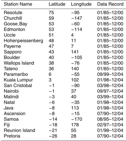
Table 1. Ozonesonde stations, locations, and data span. The table gives the names of the
stations providing data used in this paper, the geographic location of the station, and the span of time of observations used in this paper.
Station Name Latitude Longitude Data Record Resolute 75 −95 01/85–12/00 Churchill 59 −147 01/85–12/00 Goose Bay 53 −60 01/85–12/00 Edmonton 53 −114 01/85–12/00 Uccle 51 4 01/85–12/00 Hohenpeissenberg 48 11 01/85–12/00 Payerne 47 7 01/85–12/00 Sapporo 43 141 01/85–12/00 Boulder 40 −105 01/85–12/00 Wallops Island 38 −76 01/85–12/00 Tateno 36 140 01/85–12/00 Paramaribo 6 −55 09/99–12/04 Kuala Lumpur 3 102 01/98–12/04 San Cristobal −1 −90 03/98–12/04 Nairobi −1 37 09/97–12/04 Malindi −3 40 03/99–12/04 Natal −6 −35 01/98–12/04 Java −8 113 01/98–12/04 Ascension −8 −15 07/90–12/04 Samoa −14 −170 08/95–12/04 Fiji −18 178 02/97–12/04 Reunion Island −21 55 01/98–12/04 Pretoria −26 28 07/90–12/04 1616