Underlying Event measurements in pp collisions at sqrt(s) = 0.9 and 7 TeV with the ALICE experiment at the LHC

Texte intégral

(1)EUROPEAN ORGANIZATION FOR NUCLEAR RESEARCH. CERN-PH-EP-2011-204 09 Dec 2011. √ Underlying Event measurements in pp collisions at s = 0.9 and 7 TeV with the ALICE experiment at the LHC. arXiv:1112.2082v4 [hep-ex] 8 Apr 2017. ALICE Collaboration∗. Abstract √ We present measurements of Underlying Event observables in pp collisions at s = 0.9 and 7 TeV. The analysis is performed as a function of the highest charged-particle transverse momentum pT,LT in the event. Different regions are defined with respect to the azimuthal direction of the leading (highest transverse momentum) track: Toward, Transverse and Away. The Toward and Away regions collect the fragmentation products of the hardest partonic interaction. The Transverse region is expected to be most sensitive to the Underlying Event activity. The study is performed with charged particles above three different pT thresholds: 0.15, 0.5 and 1.0 GeV/c. In the Transverse region we observe an increase in the multiplicity of a factor 2-3 between the lower and higher collision energies, depending on the track pT threshold considered. Data are compared to P YTHIA 6.4, P YTHIA 8.1 and P HOJET. On average, all models considered underestimate the multiplicity and summed pT in the Transverse region by about 10-30%.. ∗ See. Appendix A for the list of collaboration members.

(2) Underlying Event measurements with ALICE. 1. ALICE Collaboration. Introduction. The detailed characterization of hadronic collisions is of great interest for the understanding of the underlying physics. The production of particles can be classified according to the energy scale of the process involved. At high transverse momentum transfers (pT & 2 GeV/c) perturbative Quantum Chromodynamics (pQCD) is the appropriate theoretical framework to describe partonic interactions. This approach can be used to quantify parton yields and correlations, whereas the transition from partons to hadrons is a non-perturbative process that has to be treated using phenomenological approaches. Moreover, the bulk of particles produced in high-energy hadronic collisions originate from low-momentum transfer processes. For momenta of the order of the QCD scale, O(100 MeV), a perturbative treatment is no longer feasible. Furthermore, at the center-of-mass energies of the Large Hadron Collider (LHC), at momentum transfers of a few GeV/c, the calculated QCD cross-sections for 2-to-2 parton scatterings exceed the total hadronic cross-section [1]. This result indicates that Multiple Partonic Interactions (MPI) occur in this regime. The overall event dynamics cannot be derived fully from first principles and must be modeled using phenomenological calculations. Measurements at different center-of-mass energies are required to test and constrain these models. In this paper, we present an analysis of the bulk particle production in pp collisions at the LHC by measuring the so-called Underlying Event (UE) activity [2]. The UE is defined as the sum of all the processes that build up the final hadronic state in a collision excluding the hardest leading order partonic interaction. This includes fragmentation of beam remnants, multiple parton interactions and initialand final-state radiation (ISR/FSR) associated to each interaction. Ideally, we would like to study the correlation between the UE and perturbative QCD interactions by isolating the two leading partons with topological cuts and measuring the remaining event activity as a function of the transferred momentum scale (Q2 ). Experimentally, one can identify the products of the hard scattering, usually the leading jet, and study the region azimuthally perpendicular to it as a function of the jet energy. Results of such an analysis have been published by the CDF [2, 3, 4, 5] and STAR [6] collaborations for pp collisions √ at s = 1.8 and 0.2 TeV, respectively. Alternatively, the energy scale is given by the leading chargedparticle transverse momentum, circumventing uncertainties related to the jet reconstruction procedure at low pT . It is clear that this is only an approximation to the original outgoing parton momentum, the exact relation depends on the details of the fragmentation mechanism. The same strategy based on the leading charged particle has recently been applied by the ATLAS [7] and CMS [8] collaborations. In the present paper we consider only charged primary particles1 , due to the limited calorimetric acceptance of the ALICE detector systems in azimuth. Distributions are measured for particles in the pseudorapidity range |η| < 0.8 with pT > pT,min , where pT,min = 0.15, 0.5 and 1.0 GeV/c, and are studied as a function of the leading particle transverse momentum. Many Monte Carlo (MC) generators for the simulation of pp collisions are available; see [9] for a recent review discussing for example P YTHIA [10], P HOJET [11], S HERPA [9] and H ERWIG [12]. These provide different descriptions of the UE associated with high energy hadron collisions. A general strategy is to combine a perturbative QCD treatment of the hard scattering with a phenomenological approach to soft processes. This is the case for the two models used in our analysis: P YTHIA and P HOJET. In P YTHIA the simulation starts with a hard LO QCD process of the type 2 → 2. Multi-jet topologies are generated with the parton shower formalism and hadronization is implemented through the Lund string fragmentation model [13]. Each collision is characterized by a different impact parameter b. Small b values correspond to a large overlap of the two incoming hadrons and to an increased probability for MPIs. At small pT values color screening effects need to be taken into account. Therefore a cut-off pT,0 is introduced, which damps the QCD cross-section for pT pT,0 . This cut-off is one of the main tunable model parameters. 1 Primary particles are defined as prompt particles produced in the collision and their decay products (strong and electromagnetic decays), except products of weak decays of strange particles such as KS0 and Λ.. 2.

(3) Underlying Event measurements with ALICE. ALICE Collaboration. In P YTHIA version 6.4 [10] MPI and ISR have a common transverse momentum evolution scale (called interleaved evolution [14]). Version 8.1 [15] is a natural extension of version 6.4, where the FSR evolution is interleaved with MPI and ISR and parton rescatterings [16] are considered. In addition initial-state partonic fluctuations are introduced, leading to a different amount of color-screening in each event. P HOJET is a two-component event generator, where the soft regime is described by the Dual Parton Model (DPM) [17] and the high-pT particle production by perturbative QCD. The transition between the two regimes happens at a pT cut-off value of 3 GeV/c. A high-energy hadronic collision is described by the exchange of effective Pomerons. Multiple-Pomeron exchanges, required by unitarization, naturally introduce MPI in the model. UE observables allow one to study the interplay of the soft part of the event with particles produced in the hard scattering and are therefore good candidates for Monte Carlo tuning. A better understanding of the processes contributing to the global event activity will help to improve the predictive power of such models. Further, a good description of the UE is needed to understand backgrounds to other observables, e.g., in the reconstruction of high-pT jets. The paper is organized in the following way: the ALICE sub-systems used in the analysis are described in Section 2 and the data samples in Section 3. Section 4 is dedicated to the event and track selection. Section 5 introduces the analysis strategy. In Sections 6 and 7 we focus on the data correction procedure and systematic uncertainties, respectively. Final results are presented in Section 8 and in Section 9 we draw conclusions.. 2. ALICE detector. Optimized for the high particle densities encountered in heavy-ion collisions, the ALICE detector is also well suited for the study of pp interactions. Its high granularity and particle identification capabilities can be exploited for precise measurements of global event properties [18, 19, 20, 21, 22, 23, 24]. The central barrel covers the polar angle range 45◦ − 135◦ (|η| < 1) and full azimuth. It is contained in the L3 solenoidal magnet which provides a nominal uniform magnetic field of 0.5 T. In this section we describe only the trigger and tracking detectors used in the analysis, while a detailed discussion of all ALICE sub-systems can be found in [25]. The V0A and V0C counters consist of scintillators with a pseudorapidity coverage of −3.7 < η < −1.7 and 2.8 < η < 5.1, respectively. They are used as trigger detectors and to reject beam–gas interactions. Tracks are reconstructed combining information from the two main tracking detectors in the ALICE central barrel: the Inner Tracking System (ITS) and the Time Projection Chamber (TPC). The ITS is the innermost detector of the central barrel and consists of six layers of silicon sensors. The first two layers, closely surrounding the beam pipe, are equipped with high granularity Silicon Pixel Detectors (SPD). They cover the pseudorapidity ranges |η| < 2.0 and |η| < 1.4 respectively. The position resolution is 12 µm in rφ and about 100 µm along the beam direction. The next two layers are composed of Silicon Drift Detectors (SDD). The SDD is an intrinsically 2-dimensional sensor. The position along the beam direction is measured via collection anodes and the associated resolution is about 50 µm. The rφ coordinate is given by a drift time measurement with a spatial resolution of about 60 µm. Due to drift field non-uniformities, which were not corrected for in the 2010 data, a systematic uncertainty of 300 µm is assigned to the SDD points. Finally, the two outer layers are made of double-sided Silicon micro-Strip Detectors (SSD) with a position resolution of 20 µm in rφ and about 800 µm along the beam direction. The material budget of all six layers including support and services amounts to 7.7% of a radiation length. The main tracking device of ALICE is the Time Projection Chamber that covers the pseudorapidity range of about |η| < 0.9 for tracks traversing the maximum radius. In order to avoid border effects, the fiducial. 3.

(4) Underlying Event measurements with ALICE. ALICE Collaboration. Collision energy: 0.9 TeV Events Offline trigger 5,515,184 Reconstructed vertex 4,482,976 Leading track pT > 0.15 GeV/c 4,043,580 Leading track pT > 0.5 GeV/c 3,013,612 Leading track pT > 1.0 GeV/c 1,281,269 Collision energy: 7 TeV Events Offline trigger 25,137,512 Reconstructed vertex 22,698,200 Leading track pT > 0.15 GeV/c 21,002,568 Leading track pT > 0.5 GeV/c 17,159,249 Leading track pT > 1.0 GeV/c 9,873,085. % of all 100.0 81.3 73.3 54.6 23.2 % of all 100.0 90.3 83.6 68.3 39.3. Table 1: Events remaining after each event selection step.. region has been restricted in this analysis to |η| < 0.8. The position resolution along the rφ coordinate varies from 1100 µm at the inner radius to 800 µm at the outer. The resolution along the beam axis ranges from 1250 µm to 1100 µm. For the evaluation of the detector performance we use events generated with the P YTHIA 6.4 [10] Monte Carlo with tune Perugia-0 [26] passed through a full detector simulation based on G EANT 3 [27]. The same reconstruction algorithms are used for simulated and real data.. 3. Data samples. √ The analysis uses two data sets which were taken at the center-of-mass energies of s = 0.9 and 7 TeV. √ In May 2010, ALICE recorded about 6 million good quality minimum-bias events at s = 0.9 TeV. The luminosity was of the order of 1026 cm−2 s−1 and, thus, the probability for pile-up events in the same √ bunch crossing was negligible. The s = 7 TeV sample of about 25 million events was collected in April 2010 with a luminosity of 1027 cm−2 s−1 . In this case the mean number of interactions per bunch crossing µ ranges from 0.005 to 0.04. A set of high pile-up probability runs (µ = 0.2 − 2) was analysed in order to study our pile-up rejection procedure and determine its related uncertainty. Those runs are excluded from the analysis. Corrected data are compared to three Monte Carlo models: P YTHIA 6.4 (tune Perugia-0), P YTHIA 8.1 (tune 1 [15]) and P HOJET 1.12.. 4 4.1. Event and track selection Trigger and offline event selection. Events are recorded if either of the three triggering systems, V0A, V0C or SPD, has a signal. The arrival time of particles in the V0A and V0C are used to reject beam–gas interactions that occur outside the nominal interaction region. A more detailed description of the online trigger can be found in [20]. An additional offline selection is made following the same criteria but considering reconstructed information instead of online trigger signals. For each event a reconstructed vertex is required. The vertex reconstruction procedure is based on tracks as well as signals in the SPD. Only vertices within ±10 cm of the nominal interaction point along the. 4.

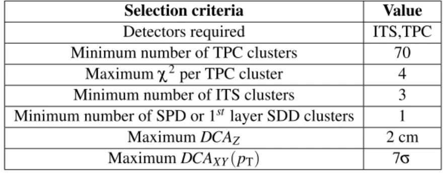
(5) Underlying Event measurements with ALICE. ALICE Collaboration. Selection criteria Detectors required Minimum number of TPC clusters Maximum χ 2 per TPC cluster Minimum number of ITS clusters Minimum number of SPD or 1st layer SDD clusters Maximum DCAZ Maximum DCAXY (pT ). Value ITS,TPC 70 4 3 1 2 cm 7σ. Table 2: Track selection criteria.. beam axis are considered. Moreover, we require at least one track with pT > pT,min = 0.15, 0.5 or 1.0 GeV/c in the acceptance |η| < 0.8. √ A pile-up rejection procedure is applied to the set of data taken at s = 7 TeV: events with more than one distinct reconstructed primary vertex are rejected. This cut has a negligible effect on simulated events without pile-up: only 0.06% of the events are removed. We have compared a selection of high pile-up probability runs (see Section 3) with a sample of low pile-up probability runs. The UE distributions differ by 20-25% between the two samples. After the above mentioned rejection procedure, the difference is reduced to less than 2%. Therefore, in the runs considered in the analysis, the effect of pile-up is negligible. No explicit rejection of cosmic-ray events is applied since cosmic particles are efficiently suppressed by our track selection cuts [23]. This is further confirmed by the absence of a sharp enhanced correlation at ∆φ = π from the leading track which would be caused by almost straight high-pT tracks crossing the detector. Table 1 summarizes the percentage of events remaining after each event selection step. We do not explicitly select non-diffractive events, although the above mentioned event selection significantly reduces the amount of diffraction in the sample. Simulated events show that the event selections reduce the fraction of diffractive events from 18-33% to 11-16% (P YTHIA 6.4 and P HOJET at 0.9 and 7 TeV). We do not correct for this contribution. 4.2. Track cuts. The track cuts are optimized to minimize the contamination from secondary tracks. For this purpose a track must have at least 3 ITS clusters, one of which has to be in the first 3 layers. Moreover, we require at least 70 (out of a maximum of 159) clusters in the TPC drift volume. The quality of the track fitting measured in terms of the χ 2 per space point is required to be lower than 4 (each space point having 2 degrees of freedom). We require the distance of closest approach of the track to the primary vertex along the beam axis (DCAZ ) to be smaller than 2 cm. In the transverse direction we apply a pT dependent DCAXY cut, corresponding to 7 standard deviations of its inclusive probability distribution. These cuts are summarized in Table 2.. 5. Analysis strategy. The Underlying Event activity is characterized by the following observables [2]: – average charged particle density vs. leading track transverse momentum pT,LT : 1 1 Nch (pT,LT ) ∆η · ∆Φ Nev (pT,LT ) 5. (1).

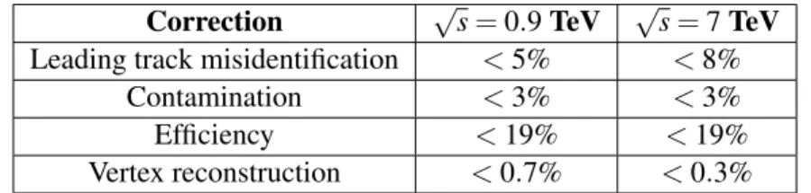
(6) Underlying Event measurements with ALICE. ALICE Collaboration. !". Fig. 1: Definition of the regions Toward, Transverse and Away w.r.t. leading track direction.. – average summed pT density vs. leading track pT,LT : 1 1 pT (pT,LT ) ∆η · ∆Φ Nev (pT,LT ) ∑. (2). – ∆φ -correlation between tracks and the leading track: 1 dNch 1 ∆η Nev (pT,LT ) d∆φ. (3). (in bins of leading track pT,LT ). Nev is the total number of events selected and Nev (pT,LT ) is the number of events in a given leading-track transverse-momentum bin. The first two variables are evaluated in three distinct regions. These regions, illustrated in Fig. 1, are defined with respect to the leading track azimuthal angle: – Toward: |∆φ | < 1/3 π – Transverse: 1/3 π < |∆φ | < 2/3 π – Away: |∆φ | > 2/3 π where ∆φ = φLT − φ is defined in ±π. In Eq. (1)-(3) the normalization factor ∆Φ is equal to 2/3π, which is the size of each region. ∆η = 1.6 corresponds to the acceptance in pseudorapidity. The leading track is not included in the final distributions.. 6. Corrections. We correct for the following detector effects: vertex reconstruction efficiency, tracking efficiency, contamination from secondary particles and leading-track misidentification bias. The various corrections are explained in more detail in the following subsections. We do not correct for the trigger efficiency since its value is basically 100% for events which have at least one particle with pT > 0.15 GeV/c in the range |η| < 0.8. In Table 3 we summarize the maximum effect of each correction on the measured final observables at the two collision energies for pT,min = 0.5 GeV/c. 6.

(7) Underlying Event measurements with ALICE. ALICE Collaboration. Correction Leading track misidentification Contamination Efficiency Vertex reconstruction. √ s = 0.9 TeV < 5% < 3% < 19% < 0.7%. √ s = 7 TeV < 8% < 3% < 19% < 0.3%. Table 3: Maximum effect of corrections on final observables for pT,min = 0.5 GeV/c.. Vertex reconstruction The correction for finite vertex reconstruction efficiency is performed as a func√ √ tion of the measured multiplicity. Its value is smaller than 0.7% and 0.3% at s = 0.9 and s = 7 TeV, respectively. Tracking efficiency The tracking efficiency depends on the track level observables η and pT . The projections of the tracking efficiency on the pT and η axes are shown in Fig. 2. In the pseudorapidity projection we observe a dip of about 1% at η = 0 due to the central TPC cathode. The slight asymmetry between positive and negative η is due to a different number of active SPD and SDD modules in the two halves of the detector. The number of active modules also differs between the data-taking periods at the two collision energies. Moreover, the efficiency decreases by 5% in the range 1-3 GeV/c. This is due to the fact that above about 1 GeV/c tracks are almost straight and can be contained completely in the dead areas between TPC sectors. Therefore, at high pT the efficiency is dominated by geometry and has a constant value of about 80% at both collision energies. To avoid statistical fluctuations, the estimated efficiency is fitted with a constant for pT > 5 GeV/c (not shown in the figure). Contamination from secondaries We correct for secondary tracks that pass the track selection cuts. Secondary tracks are predominantly produced by weak decays of strange particles (e.g. KS0 and Λ), photon conversions or hadronic interactions in the detector material, and decays of charged pions. The relevant track level observables for the contamination correction are transverse momentum and pseudorapidity. The correction is determined from detector simulations and is found to be 15-20% for tracks with pT < 0.5 GeV/c and saturates at about 2% for higher transverse momenta (see Fig. 3). We multiply the contamination estimate by a data-driven coefficient to take into account the low strangeness yield in the Monte Carlo compared to data [24]. The coefficient is derived from a fit of the discrepancy between data and Monte Carlo strangeness yields in the tails of the DCAXY distribution which are predominantly populated by secondaries. The factor has a maximum value of 1.07 for tracks with pT < 0.5 GeV/c and is equal to 1 for pT > 1.5 GeV/c. This factor is included in the Contamination entry in Table 3. Leading-track misidentification Experimentally, the real leading track can escape detection because of tracking inefficiency and the detector’s finite acceptance. In these cases another track (i.e. the subleading or sub-sub-leading etc.) will be selected as the leading one, thus biasing the analysis in two possible ways. Firstly, the sub-leading track will have a different transverse momentum than the leading one. We refer to this as leading-track pT bin migration. It has been verified with Monte Carlo that this effect is negligible due to the weak dependence of the final distributions on pT,LT . Secondly, the reconstructed leading track might have a significantly different orientation with respect to the real one, resulting in a rotation of the overall event topology. The largest bias occurs when the misidentified leading track falls in the Transverse region defined by the real leading track. We correct for leading-track misidentification with a data-driven procedure. Starting from the measured distributions, for each event the track loss due to inefficiency is applied a second time to the data (having been applied the first time naturally by the detector) by rejecting tracks randomly. If the leading track is considered reconstructed it is used as before to define the different regions. Otherwise the sub-leading. 7.

(8) ALICE Collaboration. 0.85. Tracking efficiency. Tracking Efficiency. Underlying Event measurements with ALICE. 0.8. 0.75. 0.8. 0.75. s = 0.9 TeV. 0.7. 1. 2. 3. 4. 5. 6. s = 0.9 TeV. 0.7. s = 7 TeV. 0.65 0. 0.85. s = 7 TeV. 0.65 7. 8. 9 10 pT (GeV/c). -1. -0.8. -0.6. -0.4. -0.2. 0. 0.2. 0.4. 0.6. 0.8. 1 η. Fig. 2: Tracking efficiency vs. track pT (left, |η| < 0.8) and η (right, pT > 0.5 GeV/c) from a P YTHIA 6.4 and G EANT 3 simulation.. track is used. Since the tracking inefficiency is quite small (about 20%) applying it on the reconstructed data a second time does not alter the results significantly. To verify this statement we compared our results with a two step procedure. In this case the inefficiency is applied two times on measured data, half of its value at a time. The correction factor obtained in this way is compatible with the one step procedure. Furthermore, the data-driven procedure has been tested on simulated data where the true leading particle is known. We observed a discrepancy between the two methods, especially at low leading-track pT values, which is taken into account in the systematic error. The maximum leading-track misidentification correction is 8% on the final distributions. Two-track effects By comparing simulated events corrected for single-particle efficiencies with the input Monte Carlo, we observe a 0.5% discrepancy around ∆φ = 0. This effect is called non-closure in Monte Carlo (it will be discussed further in Section 7) and in this case is related to small two-track resolution effects. Data are corrected for this discrepancy.. 7. Systematic uncertainties. In Tables 4, 5 and 6 we summarize the systematic uncertainties evaluated in the analysis for the three track thresholds: pT > 0.15, 0.5 and 1.0 GeV/c. Each uncertainty is explained in more detail in the following subsections. Uncertainties which are constant as a function of leading-track pT are listed in Table 4. √ Leading-track pT dependent uncertainties are summarized in Tables 5 and 6 for s = 0.9 TeV and 7 TeV, respectively. Positive and negative uncertainties are propagated separately, resulting in asymmetric final uncertainties. Particle composition The tracking efficiency and contamination corrections depend slightly on the particle species mainly due to their decay length and absorption in the material. To assess the effect of an incorrect description of the particle abundances in the Monte Carlo, we varied the relative yields of pions, protons, kaons, and other particles by 30% relative to the default Monte Carlo predictions. The maximum variation of the final values is 0.9% and represents the systematic uncertainty related to the particle composition (see Table 4). Moreover, we have compared our assessment of the underestimation of strangeness yields with a direct measurement from the ALICE collaboration [24]. Based on the discrepancy between the two estimates, we assign a systematic uncertainty of 0-2.3% depending on the pT threshold and collision energy, see Tables 5 and 6.. 8.

(9) ALICE Collaboration. Correction Factor. Correction Factor. Underlying Event measurements with ALICE. 1 0.98 0.96. 0.984 0.982 0.98. 0.94 0.978 0.92 0.976 0.9. s = 0.9 TeV. s = 0.9 TeV 0.974. 0.88. s = 7 TeV. 0.86 0.84 0. 1. 2. 3. 4. 5. 6. 7. 8. s = 7 TeV. 0.972 0.97 -1. 9 10 pT (GeV/c). -0.8. -0.6. -0.4. -0.2. 0. 0.2. 0.4. 0.6. 0.8. 1 η. Fig. 3: Contamination correction: correction factor vs. track pT (left, |η| < 0.8) and η (right, pT > 0.5 GeV/c) from a P YTHIA 6.4 and G EANT 3 simulation.. Particle composition ITS efficiency TPC efficiency Track cuts ITS/TPC matching MC dependence Material budget. Particle composition ITS efficiency TPC efficiency Track cuts ITS/TPC matching MC dependence Material budget. √ s = 0.9 TeV pT > 0.5 GeV/c ± 0.7% – ± 0.8%. pT > 0.15 GeV/c ± 0.9% ± 0.6% ± 1.9%. pT > 1.0 GeV/c ± 0.4% – ± 0.4%. + 3.0% − 1.1%. + 2.0% − 1.1%. + 0.9% − 1.5%. ± 1.0% + 1.1% , + 1.1% , + 1.6% ± 0.6%. ± 1.0% + 0.9% , + 0.9% , + 1.3% ± 0.2%. pT > 0.15 GeV/c ± 0.9% ± 0.5% ± 1.8%. ± 1.0% + 0.9% ± 0.2% √ s = 7 TeV pT > 0.5 GeV/c ± 0.7% – ± 0.8%. + 2.1% − 2.3%. + 1.6% − 3.2%. + 2.5% − 3.5%. ± 1.0% + 0.8% , + 0.8% , + 1.2% ± 0.6%. ± 1.0% + 0.8% ± 0.2%. ± 1.0% + 1.0% ± 0.2%. pT > 1.0 GeV/c ± 0.5% – ± 0.5%. Table 4: Constant systematic uncertainties at both collision energies. When more than one number is quoted, separated by a comma, the first value refers to the number density distribution, the second to the summed pT and the third to the azimuthal correlation. Some of the uncertainties are quoted asymmetrically.. ITS and TPC efficiency The tracking efficiency depends on the level of precision of the description of the ITS and TPC detectors in the simulation and the modeling of their response. After detector alignment with survey methods, cosmic-ray events and pp collision events [28], the uncertainty on the efficiency due to the ITS description is estimated to be below 2% and affects only tracks with pT < 0.3 GeV/c. The uncertainty due to the TPC reaches 4.5% at very low pT and is smaller than 1.2% for tracks with pT > 0.5 GeV/c. The resulting maximum uncertainty on the final distributions is below 1.9%. Moreover, an uncertainty of 1% is included to account for uncertainties in the MC description of the matching between TPC and ITS tracks (see Table 4). Track cuts By applying the efficiency and contamination corrections we correct for those particles which are lost due to detector effects and for secondary tracks which have not been removed by the selection cuts. These corrections rely on detector simulations and therefore, one needs to estimate the systematic uncertainty introduced in the correction procedure by one particular choice of track cuts. To do so, we repeat the analysis with different values of the track cuts, both for simulated and real data. The 9.

(10) Underlying Event measurements with ALICE. ALICE Collaboration. variation of the final distributions with different track cuts is a measure of the systematic uncertainty. The overall effect, considering all final distributions, is smaller than 3.5% at both collision energies (see Table 4). Misidentification bias The uncertainty on the leading-track misidentification correction is estimated from the discrepancy between the data-driven correction used in the analysis and that based on simulations. The effect influences only the first two leading-track pT bins at both collision energies. The maximum uncertainty (∼ 18%) affects the first leading-track pT bin for the track pT cut-off of 0.15 GeV/c. In all other bins this uncertainty is of the order of few percent. As summarized in Tables 5 and 6, the uncertainty has slightly different values for the various UE distributions. Vertex-reconstruction efficiency The analysis accepts reconstructed vertices with at least one contributing track. We repeat the analysis requiring at least two contributing tracks. The systematic uncertainty related to the vertex reconstruction efficiency is given by the maximum variation in the final distributions between the cases of one and two contributing tracks. Its value is 2.4% for pT,min = 0.15 GeV/c and below 1% for the other cut-off values (see Tables 5 and 6). The effect is only visible in the first leading-track pT bin. Non-closure in Monte Carlo By correcting a Monte Carlo prediction after full detector simulation with corrections extracted from the same generator, we expect to obtain the input Monte Carlo prediction within the statistical uncertainty. This consideration holds true only if each correction is evaluated with respect to all the variables to which the given correction is sensitive. Any statistically significant difference between input and corrected distributions is referred to as non-closure in Monte Carlo. The overall non-closure effect is sizable (∼ 17%) in the first leading-track pT bin and is 0.6-5.3% in all other bins at both collision energies. Monte-Carlo dependence The difference in final distributions when correcting the data with P YTHIA 6.4 or P HOJET generators is of the order of 1% and equally affects all the leading-track pT bins. Material budget The material budget has been measured by reconstructing photon conversions which allows a precise γ-ray tomography of the ALICE detector. For the detector regions important for this analysis the remaining uncertainty on the extracted material budget is less than 7%. Varying the material density in the detector simulation, the effect on the observables presented is determined to be 0.2-0.6% depending on the pT threshold considered.. 8. Results. In this section we present and discuss the corrected results for the three UE distributions in all regions at the two collision energies. The upper part of each plot shows the relevant measured distribution (black points) compared to a set of Monte Carlo predictions (coloured curves). Shaded bands represent the systematic uncertainty only. Error bars along the x axis indicate the bin width. The lower part shows the ratio between Monte Carlo and data. In this case the shaded band is the sum in quadrature of statistical and systematic uncertainties. The overall agreement of data and simulations is of the order of 10-30% and we were not able to identify a preferred model that can reproduce all measured observables. In general, all three generators underestimate the event activity in the Transverse region. Nevertheless, an agreement of the order of 20% has to be considered a success, considering the complexity of the system under study. Even though an exhaustive comparison of data with the latest models available is beyond the scope of this paper, in the next sections we will indicate some general trends observed in the comparison with the chosen models.. 10.

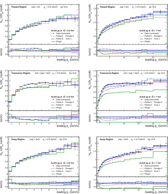
(11) Underlying Event measurements with ALICE. Lead. track misid. MC non closure. Strangeness Vertex reco.. Lead. track misid. MC non closure. Strangeness Vertex reco.. Lead. track misid. MC non closure. Strangeness Vertex reco.. pT,LT 1st bin 2nd bin 1st bin 2nd bin others 1st bin others 1st bin pT,LT 1st bin 2nd bin 1st bin 2nd bin others 1st bin others 1st bin pT,LT 1st bin 2nd bin 1st bin 2nd bin others 1st bin others 1st bin others. ALICE Collaboration. √ s = 0.9 TeV Number density pT > 0.15 GeV/c pT > 0.5 GeV/c + (17.8, 16.3, 16.3)% + (4.6, 3.5, 3.5)% + 2.9% + 1.3% − 17.2% − 3.6% − 3.2% − 0.8% − 0.6% − 0.8% ± 1.9% ± 0.2% ± 1.0% ± 0.2% − 2.4% − 0.7% Summed pT pT > 0.15 GeV/c pT > 0.5 GeV/c + (20.0, 18.1, 18.1)% + (5.3, 4.1, 4.1)% + 3.7% + 1.6% − 17.0% − 2.8% − 3.0% − 1.0% − 0.7% − 1.0% ± 1.9% ± 0.2% ± 1.0% ± 0.2% − 2.4% − 0.7% Azimuthal correlation pT > 0.15 GeV/c pT > 0.5 GeV/c + 12.0% + 3.9% + 2.6% + 1.1% − 17.1% − 3.3% − 3.5% − 3.0% − 2.4% − 3.0% ± 1.9% ± 0.2% ± 1.0% ± 0.2% − 2.4% − 0.4% − 0.5% − 0.4%. pT > 1.0 GeV/c + (4.2, 2.9, 1.7)% – − 1.2% − 1.2% − 1.2% – – − 0.5% pT > 1.0 GeV/c + (4.8, 3.4, 3.4)% – − 1.1% − 1.1% − 1.1% – – − 0.5% pT > 1.0 GeV/c + 2.5% – − 1.6% − 1.6% − 1.6% – – – –. √ Table 5: Systematic uncertainties vs. leading track pT at s = 0.9 TeV. When more than one number is quoted, separated by a comma, the first value refers to the Toward, the second to the Transverse and the third to the Away region. The second column denotes the leading track pT bin for which the uncertainty applies. The numbering starts for each case from the first bin above the track pT threshold.. In the following discussion we define the leading track pT range from 4 to 10 GeV/c at √ and from 10 to 25 GeV/c at s = 7 TeV as the plateau. 8.1. √ s = 0.9 TeV. Number density. In Fig. 4-6 we show the multiplicity density as a function of leading track pT in the three regions: Toward, Transverse and Away. Toward and Away regions are expected to collect the fragmentation products of the two back-to-back outgoing partons from the elementary hard scattering. We observe that the multiplicity density in these regions increases monotonically with the pT,LT scale. In the Transverse region, after a monotonic increase at low leading track pT , the distribution tends to flatten out. The same behaviour is observed at both collision energies and all values of pT,min . The rise with pT,LT has been interpreted as evidence for an impact parameter dependence in the hadronic collision [29]. More central collisions have an increased probability for MPI, leading to a larger transverse multiplicity. Nevertheless, we must be aware of a trivial effect also contributing to the low pT,LT region. For instance for any probability distribution, the maximum value per randomized sample averaged over many samples rises steadily with the sample size M. In our case, the conditional probability density P(pT,LT |M) shifts towards larger pT,LT with increasing M. Using Bayes’ theorem one expects 11.

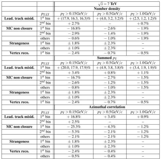
(12) Underlying Event measurements with ALICE. Lead. track misid. MC non closure. Strangeness Vertex reco.. Lead. track misid. MC non closure. Strangeness Vertex reco.. Lead. track misid. MC non closure. Strangeness Vertex reco.. pT,LT 1st bin 2nd bin 1st bin 2nd bin others 1st bin others 1st bin pT,LT 1st bin 2nd bin 1st bin 2nd bin others 1st bin others 1st bin pT,LT 1st bin 2nd bin 1st bin 2nd bin others 1st bin others 1st bin others. ALICE Collaboration. √ s = 7 TeV Number density pT > 0.15 GeV/c pT > 0.5 GeV/c + (17.9, 16.3, 16.3)% + (4.0, 3.2, 3.2)% + 2.7% – − 16.8% − 2.6% − 2.9% − 1.4% − 0.6% − 1.0% ± 1.8% ± 2.3% ± 1.0% ± 2.3% − 2.4% − 0.7% Summed pT pT > 0.15 GeV/c pT > 0.5 GeV/c + (20.0, 17.9, 17.9)% + (4.9, 3.8, 3.8)% + 3.4% + 0.8% − 16.7% − 2.7% − 2.6% − 1.2% − 0.8% − 1.0% ± 1.8% ± 2.3% ± 1.0% ± 2.3% − 2.4% − 0.7% Azimuthal correlation pT > 0.15 GeV/c pT > 0.5 GeV/c + 16.8% + 3.4% + 2.5% – − 25.3% − 4.3% − 5.3% − 2.1% − 2.1% − 2.1% ± 1.8% ± 2.3% ± 1.0% ± 2.3% − 2.4% − 0.4% − 0.5% − 0.4%. pT > 1.0 GeV/c + (2.5, 1.2, 1.2)% + 0.7% − 1.9% − 1.9% − 1.9% – – − 0.5% pT > 1.0 GeV/c + (3.4, 1.9, 1.9)% + 1.1% − 1.5% − 1.5% − 1.5% – – − 0.5% pT > 1.0 GeV/c + 0.9% – − 1.2% − 1.2% − 1.2% – – – –. √ Table 6: Systematic uncertainties vs. leading track pT at s = 7 TeV. When more than one number is quoted, separated by a comma, the first value refers to the Toward, the second to the Transverse and the third to the Away region. The second column denotes the leading track pT bin for which the uncertainty applies. The numbering starts for each case from the first bin above the track pT threshold.. the conditional probability density P(M|pT,LT ) to shift towards larger M with rising pT,LT : P(M|pT,LT ) ∼ P(pT,LT |M)P(M).. (4). The saturation of the distribution at higher values of pT,LT indicates the onset of the event-by-event partitioning into azimuthal regions containing the particles from the hard scattering and the UE region. The bulk particle production becomes independent of the hard scale. The plateau range is fitted with a line. The fit slopes, consistent with zero, and mean values for the three pT thresholds are reported in Table 7. In the fit, potential correlations of the systematic uncertainties in different pT bins are neglected. ATLAS has published a UE measurement where the hard scale is given by the leading track pT , with a pT threshold for particles of 0.5 GeV/c and an acceptance of |η| < 2.5 [7]. Given the different acceptance with respect to our measurement, the results in the Toward and Away regions are not comparable. On the other hand the mean values of the Transverse plateaus from the two measurements are in good agreement, indicating an independence of the UE activity on the pseudorapidity range. The CDF collaboration measured the UE as a function of charged particle jet pT at a collision energy of 1.8 TeV[2]. The particle 12.

(13) Underlying Event measurements with ALICE. ALICE Collaboration √ s = 0.9 TeV. pT > 0.15 GeV/c pT > 0.5 GeV/c pT > 1.0 GeV/c. pT > 0.15 GeV/c pT > 0.5 GeV/c pT > 1.0 GeV/c. pT > 0.5 GeV/c. Number density Summed pT −1 Slope (GeV/c) Mean Slope Mean (GeV/c) 0.00 ± 0.02 1.00 ± 0.04 0.00 ± 0.01 0.62 ± 0.02 0.00 ± 0.01 0.45 ± 0.02 0.01 ± 0.01 0.45 ± 0.02 0.003 ± 0.003 0.16 ± 0.01 0.006 ± 0.005 0.24 ± 0.01 √ s = 7 TeV Number density Summed pT Slope (GeV/c)−1 Mean Slope Mean (GeV/c) 0.00 ± 0.01 1.82 ± 0.06 0.01 ± 0.01 1.43 ± 0.05 0.005 ± 0.007 0.95 ± 0.03 0.01 ± 0.01 1.15 ± 0.04 0.001 ± 0.003 0.41 ± 0.01 0.008 ± 0.006 0.76 ± 0.03 √ s = 1.8 TeV (CDF) Number density (at leading charged jet pT = 20 GeV/c) 0.60. Table 7: Saturation values in the Transverse region for the two collision energies. The result from CDF is also given, for details see text.. pT threshold is 0.5 GeV/c and the acceptance |η| < 1. In the Transverse region CDF measures 3.8 charged particles per unit pseudorapidity above the pT threshold at leading-jet pT = 20 GeV/c. This number needs to be divided by 2π in order to be compared with the average number of particles in the plateau from Table 7 at the same threshold value. The scaled CDF result is 0.60, also shown in Table 7 √ √ for comparison. As expected it falls between our two measurements at s = 0.9 TeV and s = 7 TeV. The values do not scale linearly with the collision energy, in particular the increase is higher from 0.9 to 1.8 TeV than from 1.8 to 7 TeV. Interpolating between our measurements assuming a logarithmic √ dependence on s results in 0.62 charged particles per unit area at 1.8 TeV, consistent with the CDF result. For illustration, Figure 7 presents the number density in the plateau of the Transverse region for pT > 0.5 GeV/c (our measurement as well as the value measured by CDF at 1.8 TeV) compared with dNch /dη|η=0 of charged particles with pT > 0.5 GeV/c in minimum-bias events [30] (scaled by 1/2π).2 The UE activity in the plateau region is more than a factor 2 larger than the dNch /dη. Both can be fitted with a logarithmic dependence on s (a + b ln s). The relative increase from 0.9 to 7 TeV for the UE is larger than that for the dNch /dη: about 110% compared to about 80%, respectively. √ √ In Fig. 8 (left) we show the ratio between the number density distribution at s = 7 TeV and s = 0.9 TeV. Most of the systematic uncertainties are expected to be correlated between the two energies, therefore we consider only statistical uncertainties. The ratio saturates for leading track pT > 4 GeV/c. The results of a constant fit in the range 4 < pT,LT < 10 GeV/c are reported in Table 8. The measured scaling factor for a pT threshold of 0.5 GeV/c is in agreement with the observations of ATLAS [7, 31] and CMS [32]. For the track threshold pT > 0.15 GeV/c all models underestimate the charged multiplicity in the Trans√ verse and Away regions. In particular at s = 7 TeV PHOJET predictions largely underestimate the measurement in the Transverse region (up to ∼ 50%), the discrepancy being more pronounced with increasing pT cut-off value. P YTHIA 8 correctly describes the Toward region at both collision energies √ and P HOJET only at s = 0.9 TeV. For track pT > 1 GeV/c, P YTHIA 8 systematically overestimates the event activity in the jet fragmentation regions (Toward and Away). 2 These. data are for events that have at least one charged particle in |η| < 2.5.. 13.

(14) Underlying Event measurements with ALICE. pT > 0.15 GeV/c pT > 0.5 GeV/c pT > 1.0 GeV/c. ALICE Collaboration. Number density 1.76 ± 0.02 1.97 ± 0.03 2.32 ± 0.04. Summed pT 2.00 ± 0.03 2.16 ± 0.03 2.48 ± 0.05. √ √ Table 8: Constant fit in 4 < pT,LT < 10 GeV/c to the ratio between s = 0.9 TeV and s = 7 TeV for number density (left) and summed pT (right) distributions in the Transverse region. The shown uncertainties are based on statistical and systematic uncertainties summed in quadrature.. 8.2. Summed pT. In Fig. 9-11 we show the summed pT density as a function of leading track pT in the three topological regions. The shape of the distributions follows a trend similar to that discussed above for the number density. The general trend of P YTHIA 8 is to overestimate the fragmentation in the Toward region at all pT cut√ off values. Also in this case at s = 7 TeV PHOJET largely underestimates the measurement in the Transverse region (up to ∼ 50%), especially at higher values of pT cut-off. Other systematic trends are not very pronounced. In Table 7 we report the mean value of a linear fit in the plateau range. Our results agree with the ATLAS measurement in the Transverse plateau. √ √ In Fig. 8 (right) we show the ratio between the distribution at s = 7 TeV and s = 0.9 TeV, considering as before only statistical errors. The results of a constant fit in the range 4 < pT,LT < 10 GeV/c are reported in Table 8. Also in this case the scaling factor is in agreement with ATLAS and CMS results. The summed pT density in the Transverse region can be interpreted as a measurement of the UE activity in a given leading track pT bin. Therefore, its value in the plateau can be used, for example, to correct jet spectra. 8.3. Azimuthal correlation. In Fig. 12-22 azimuthal correlations between tracks and the leading track are shown in different ranges of leading track pT . The range 1/3π < |∆φ | < 2/3π corresponds to the Transverse region. The regions −1/3π < ∆φ < 1/3π (Toward) and 2/3π < |∆φ | < π (Away) collect the fragmentation products of the leading and sub-leading jets. In general, all Monte Carlo simulations considered fail to reproduce the shape of the measured distributions. P YTHIA 8 provides the best prediction for the Transverse activity in all leading track pT ranges considered. Unfortunately the same model significantly overestimates the jet fragmentation regions.. 9. Conclusions. √ We have characterized the Underlying Event in pp collisions at s = 0.9 and 7 TeV by measuring the number density, the summed pT distribution and the azimuthal correlation of charged particles with √ respect to the leading particle. The analysis is based on about 6 · 106 minimum bias events at s = √ 0.9 TeV and 25 · 106 events at s = 7 TeV collected during the data taking periods from April to July 2010. Measured data have been corrected for detector related effects; in particular we applied a datadriven correction to account for the misidentification of the leading track. The fully corrected final distributions are compared with P YTHIA 6.4, P YTHIA 8 and P HOJET, showing that pre-LHC tunes have difficulties describing the data. These results are an important ingredient in the required retuning of those generators.. 14.

(15) Underlying Event measurements with ALICE. ALICE Collaboration. Among the presented distributions, the Transverse region is particularly sensitive to the Underlying √ Event. We find that the ratio between the distributions at s = 0.9 and 7 TeV in this region saturates at a value of about 2 for track pT > 0.5 GeV/c. The summed pT distribution rises slightly faster as a function √ of s than the number density distribution, indicating that the available energy tends to increase the particle’s transverse momentum in addition to the multiplicity. This is in qualitative agreement with an √ increased relative contribution of hard processes to the Underlying Event with increasing s. Moreover, the average number of particles at large pT,LT in the Transverse region seems to scale logarithmically with the collision energy. In general our results are in good qualitative and quantitative agreement with measurements from other LHC experiments (ATLAS and CMS) and show similar trends to that of the Tevatron (CDF). Our results show that the activity in the Transverse region increases logarithmically and faster than dNch /dη in minimum-bias events. Models aiming to correctly reproduce these minimum-bias and underlying event distributions need a precise description of the interplay of the hard process, the associated initial and final-state radiation and multiple parton interactions.. 15.

(16) Underlying Event measurements with ALICE. ALICE Collaboration. |∆φ| < π/3. Toward Region. pT > 0.15 GeV/c. 2. Nch 1/(Nev∆η∆Φ). Nch 1/(Nev∆η∆Φ). Number Density - track pT > 0.15 GeV/c |η| <0.8. 1.5. 1. pT > 0.15 GeV/c. 3.5 3 2.5. 2. 3. 4. 5. 6. 7. 8. 9. 0.5 0. 10. 1.2. leading p (GeV/c) T. 0.8. 1. 2. 3. 4. 5. 6. 7. 8. ALICE pp at s = 7 TeV Data (corrected) Pythia 6 - Perugia 0 Pythia 8 - Tune 1 Phojet. 1. RATIO. 1. 1. 9. 5. 10. 15. 5. 10. 15. 25 T. |η| <0.8. pT > 0.15 GeV/c. 20. leading p (GeV/c). Nch 1/(Nev∆η∆Φ). Nch 1/(Nev∆η∆Φ). π/3 < |∆φ| < 2π/3. 25. T. 0.8. 10. T. Transverse Region. 20. leading p (GeV/c). 1. leading p (GeV/c). 1.4. |η| <0.8. 2. 0. RATIO. |∆φ| < π/3. Toward Region. 4. 1.5. ALICE pp at s = 0.9 TeV Data (corrected) Pythia 6 - Perugia 0 Pythia 8 - Tune 1 Phojet. 0.5. 1.2. 4.5. 1.2 1 0.8. 3. Transverse Region. π/3 < |∆φ| < 2π/3. |η| <0.8. pT > 0.15 GeV/c. 2.5 2 1.5. 0.6. 0. RATIO. 1. 2. 3. 4. 5. 6. 7. 8. 9. 0. 10. 1.2. leading p (GeV/c). 1. T. 0.8. 1. 2. 3. 4. 5. 6. 7. 8. 9. ALICE pp at s = 7 TeV Data (corrected) Pythia 6 - Perugia 0 Pythia 8 - Tune 1 Phojet. 0.5. RATIO. 0.2. 1.2. 1. ALICE pp at s = 0.9 TeV Data (corrected) Pythia 6 - Perugia 0 Pythia 8 - Tune 1 Phojet. 0.4. 5. 10. 15. 5. 10. 15. pT > 0.15 GeV/c. |η| <0.8. 1.5. 1. Away Region. |∆φ| > 2π/3. pT > 0.15 GeV/c. |η| <0.8. 3 2.5. 1.5. ALICE pp at s = 0.9 TeV Data (corrected) Pythia 6 - Perugia 0 Pythia 8 - Tune 1 Phojet. 1. 2. 3. 4. 5. 6. 7. 8. 9. 0.5 0. 10. 1.2. leading p (GeV/c). 1. T. 0.8. 1. 2. 3. 4. 5. 6. 7. 8. 9. ALICE pp at s = 7 TeV Data (corrected) Pythia 6 - Perugia 0 Pythia 8 - Tune 1 Phojet. 1. RATIO. 0. RATIO. 4 3.5. 2. 0.5. 1.2. 25 T. Nch 1/(Nev∆η∆Φ). Nch 1/(Nev∆η∆Φ). |∆φ| > 2π/3. 20. leading p (GeV/c). T. Away Region. 25. T. 0.8. 10. leading p (GeV/c). 2. 20. leading p (GeV/c). 1. 10. 5. 15. 20. 25. leading p (GeV/c) T. 0.8. 5. leading p (GeV/c). 10. 1. 10. 15. 20. 25. leading p (GeV/c). T. T. √ Fig. 4: Number density in Toward (top), Transverse (middle) and Away (bottom) regions at s = 0.9 TeV (left) √ and s = 7 TeV (right). Right and left vertical scales differ by a factor 2. Shaded area in upper plots: systematic uncertainties. Shaded areas in bottom plots: sum in quadrature of statistical and systematic uncertainties. Horizontal error bars: bin width.. 16.

(17) Underlying Event measurements with ALICE. ALICE Collaboration. 1.4. |∆φ| < π/3. Toward Region. pT > 0.5 GeV/c. Nch 1/(Nev∆η∆Φ). Nch 1/(Nev∆η∆Φ). Number Density - track pT > 0.5 GeV/c |η| <0.8. 1.2 1 0.8. 2.5. |∆φ| < π/3. Toward Region. pT > 0.5 GeV/c. |η| <0.8. 2. 1.5. 0.6. 0. RATIO. 1. 2. 3. 4. 5. 6. 7. 8. 9. 0. 10. 1.2. leading p (GeV/c). 1. T. 0.8. 1. 2. 3. 4. 5. 6. 7. 8. 9. ALICE pp at s = 7 TeV Data (corrected) Pythia 6 - Perugia 0 Pythia 8 - Tune 1 Phojet. 0.5. RATIO. 0.2. 1.2. 1. ALICE pp at s = 0.9 TeV Data (corrected) Pythia 6 - Perugia 0 Pythia 8 - Tune 1 Phojet. 0.4. 5. 10. 15. 20 T. 0.8. 10. 5. 10. 15. 20. leading p (GeV/c). π/3 < |∆φ| < 2π/3. Nch 1/(Nev∆η∆Φ). Nch 1/(Nev∆η∆Φ). T. 0.7. Transverse Region. |η| <0.8. pT > 0.5 GeV/c. 0.5 0.4 0.3 ALICE pp at s = 0.9 TeV Data (corrected) Pythia 6 - Perugia 0 Pythia 8 - Tune 1 Phojet. Transverse Region. π/3 < |∆φ| < 2π/3. 0. 1. 2. 3. 4. 5. 6. 1 0.8. 7. 8. 9. 0. 10. 1.2. T. 0.8. 2. 3. 4. 5. 6. 7. 8. 9. ALICE pp at s = 7 TeV Data (corrected) Pythia 6 - Perugia 0 Pythia 8 - Tune 1 Phojet. 0.2. leading p (GeV/c). 1. 1. 5. 10. 15. 5. 10. 15. |η| <0.8. pT > 0.5 GeV/c. 25 T. Nch 1/(Nev∆η∆Φ). |∆φ| > 2π/3. Away Region. 20. leading p (GeV/c). T. 1.2. 25. T. 0.8. 10. 20. leading p (GeV/c). 1. leading p (GeV/c). Nch 1/(Nev∆η∆Φ). |η| <0.8. pT > 0.5 GeV/c. 1.2. 0.4. RATIO. 0.1. RATIO. 1.4. 0.6. 0.2. 1.2. 25. leading p (GeV/c). T. 0.6. 25. leading p (GeV/c). 1. 1 0.8 0.6. Away Region. |∆φ| > 2π/3. pT > 0.5 GeV/c. |η| <0.8. 2. 1.5. 1 0.4. ALICE pp at s = 0.9 TeV Data (corrected) Pythia 6 - Perugia 0 Pythia 8 - Tune 1 Phojet. 0. RATIO. 1.2. 1. 2. 3. 4. 5. 6. 7. 8. 9. 0. 10. 1.2. leading p (GeV/c). 1. T. 0.8. 1. 2. 3. 4. 5. 6. 7. 8. 9. ALICE pp at s = 7 TeV Data (corrected) Pythia 6 - Perugia 0 Pythia 8 - Tune 1 Phojet. 0.5. RATIO. 0.2. 10. 5. 15. 20. 25. leading p (GeV/c) T. 0.8. 5. leading p (GeV/c). 10. 1. 10. 15. 20. 25. leading p (GeV/c). T. T. √ Fig. 5: Number density in Toward (top), Transverse (middle) and Away (bottom) regions at s = 0.9 TeV (left) √ and s = 7 TeV (right). Right and left vertical scales differ by a factor 2. Shaded area in upper plots: systematic uncertainties. Shaded areas in bottom plots: sum in quadrature of statistical and systematic uncertainties. Horizontal error bars: bin width.. 17.

(18) Underlying Event measurements with ALICE. ALICE Collaboration. 0.8. |∆φ| < π/3. Toward Region. pT > 1.0 GeV/c. Nch 1/(Nev∆η∆Φ). Nch 1/(Nev∆η∆Φ). Number Density - track pT > 1.0 GeV/c |η| <0.8. 0.7 0.6 0.5 0.4. 0. RATIO. 2. 3. 4. 5. 6. 1. 7. 8. 9. 0. 10. 1.2. T. 0.8. 2. 3. 4. 5. 6. 7. 8. 9. ALICE pp at s = 7 TeV Data (corrected) Pythia 6 - Perugia 0 Pythia 8 - Tune 1 Phojet. 0.2. leading p (GeV/c). 1. 5. 10. 15. 20 T. 0.8. 10. 5. 10. 15. 20 T. Nch 1/(Nev∆η∆Φ). 0.3. π/3 < |∆φ| < 2π/3. |η| <0.8. pT > 1.0 GeV/c. 25. leading p (GeV/c). T. Transverse Region. 25. leading p (GeV/c). 1. leading p (GeV/c). Nch 1/(Nev∆η∆Φ). |η| <0.8. 1.2. 0.4. RATIO. 0.1. 1. pT > 1.0 GeV/c. 0.6. ALICE pp at s = 0.9 TeV Data (corrected) Pythia 6 - Perugia 0 Pythia 8 - Tune 1 Phojet. 0.2. 1. |∆φ| < π/3. Toward Region. 1.4. 0.8. 0.3. 1.2. 1.6. 0.25 0.2 0.15. 0.6. Transverse Region. π/3 < |∆φ| < 2π/3. |η| <0.8. pT > 1.0 GeV/c. 0.5 0.4 0.3. 0.1 0.2 ALICE pp at s = 0.9 TeV Data (corrected) Pythia 6 - Perugia 0 Pythia 8 - Tune 1 Phojet. 0 -0.05. 1. RATIO. 1.2. 2. 3. 4. 5. 6. 7. 8. 10. 1.2. T. 0.8. 1. 9. 0. leading p (GeV/c). 1. 2. 3. 4. 5. 6. 7. 8. 9. ALICE pp at s = 7 TeV Data (corrected) Pythia 6 - Perugia 0 Pythia 8 - Tune 1 Phojet. 0.1. RATIO. 0.05. 5. 10. 15. 5. 10. 15. 20. leading p (GeV/c). |∆φ| > 2π/3. pT > 1.0 GeV/c. T. Nch 1/(Nev∆η∆Φ). Nch 1/(Nev∆η∆Φ). Away Region. |η| <0.8. 0.5 0.4 0.3 ALICE pp at s = 0.9 TeV Data (corrected) Pythia 6 - Perugia 0 Pythia 8 - Tune 1 Phojet. 0. RATIO. 2. 3. 4. 5. 6. |∆φ| > 2π/3. pT > 1.0 GeV/c. |η| <0.8. 1 0.8. 7. 8. 9. 0. 10. 1.2. T. 0.8. 2. 3. 4. 5. 6. 7. 8. 9. ALICE pp at s = 7 TeV Data (corrected) Pythia 6 - Perugia 0 Pythia 8 - Tune 1 Phojet. 0.2. leading p (GeV/c). 1. 1. Away Region. 0.4. RATIO. 0.1. 1. 1.2. 0.6. 0.2. 1.2. 25. leading p (GeV/c). T. 0.6. 25. T. 0.8. 10. 20. leading p (GeV/c). 1. 10. 5. 15. 20. 25. leading p (GeV/c) T. 0.8. 5. leading p (GeV/c). 10. 1. 10. 15. 20. 25. leading p (GeV/c). T. T. √ Fig. 6: Number density in Toward (top), Transverse (middle) and Away (bottom) regions at s = 0.9 TeV (left) √ and s = 7 TeV (right). Right and left vertical scales differ by a factor 2. Shaded area in upper plots: systematic uncertainties. Shaded areas in bottom plots: sum in quadrature of statistical and systematic uncertainties. Horizontal error bars: bin width.. 18.

(19) Multiplicity. Underlying Event measurements with ALICE. ALICE Collaboration. MB dNch/dη (scaled by 1/2π). 1.0. Underlying Event. 0.9 0.8 0.7 0.6 0.5 0.4 0.3 0.2 0.1 8×10-1. 2. 1. 3. 4. 5. 6. 7 8 9 10 s (TeV). Fig. 7: Comparison of number density in the plateau of the Transverse region (see Table 8) and dNch /dη in minimum-bias events (scaled by 1/2π) [30]. Both are for charged particles with pT > 0.5 GeV/c. For this plot, statistical and systematic uncertainties have been summed in quadrature. The lines show fits with the functional form a + b ln s.. Summed pT ratio between 7 and 0.9 TeV in Transverse region. 3.5. RATIO. RATIO. Number density ratio between 7 and 0.9 TeV in Transverse region. 3.5. 3. 3. 2.5. 2.5. 2. 2. 1.5. 1.5 Track p threshold T p > 0.15 GeV/c T p > 0.5 GeV/c T p > 1.0 GeV/c. 1. Track p threshold T p > 0.15 GeV/c T p > 0.5 GeV/c T p > 1.0 GeV/c. 1. T. 0.5 0. 1. 2. 3. 4. 5. 6. T. 0.5 0. 7 8 9 10 Leading p (GeV/c) T. 1. 2. 3. 4. 5. 6. 7 8 9 10 Leading p (GeV/c) T. √ √ Fig. 8: Ratio between s = 0.9 TeV and s = 7 TeV for number density (left) and summed pT (right) distributions in the Transverse region. Statistical uncertainties only.. 19.

(20) Underlying Event measurements with ALICE. ALICE Collaboration. 2. |∆φ| < π/3. Toward Region. pT > 0.15 GeV/c. Σ pT 1/(Nev∆η∆Φ) (GeV/c). Σ pT 1/(Nev∆η∆Φ) (GeV/c). Summed pT - track pT > 0.15 GeV/c |η| <0.8. 1.5. 1 ALICE pp at s = 0.9 TeV Data (corrected) Pythia 6 - Perugia 0 Pythia 8 - Tune 1 Phojet. 0.5. 0. 8. |∆φ| < π/3. Toward Region. pT > 0.15 GeV/c. |η| <0.8. 7 6 5 4 3. ALICE pp at s = 7 TeV Data (corrected) Pythia 6 - Perugia 0 Pythia 8 - Tune 1 Phojet. 2 1 0. 1. 2. 3. 4. 5. 6. 7. 8. 9. 10. 1.2. RATIO. RATIO. 1.2. leading p (GeV/c). 1. T. 0.8. 1. 2. 3. 4. 5. 6. 7. 8. 9. 5. 10. 15. 5. 10. 15. Σ pT 1/(Nev∆η∆Φ) (GeV/c). 0.8. 0.6. 0.4 ALICE pp at s = 0.9 TeV Data (corrected) Pythia 6 - Perugia 0 Pythia 8 - Tune 1 Phojet. 0.2. 0. 1.2. RATIO. |η| <0.8. pT > 0.15 GeV/c. 1. 2. 3. 4. 5. 6. 7. 8. 9. 1. 2. 3. 4. 5. 6. 7. 8. 9. Transverse Region. π/3 < |∆φ| < 2π/3. 1. ALICE pp at s = 7 TeV Data (corrected) Pythia 6 - Perugia 0 Pythia 8 - Tune 1 Phojet. 0.5. 5. 10. 15. 5. 10. 15. 1 ALICE pp at s = 0.9 TeV Data (corrected) Pythia 6 - Perugia 0 Pythia 8 - Tune 1 Phojet. 0 1.2. RATIO. |η| <0.8. 1.5. 0.5. 1. 2. 3. 4. 5. 6. 7. 8. 9. 1. 2. 3. 4. 5. 6. 7. 8. 9. Away Region 4. |∆φ| > 2π/3. 3. 2 1.5. ALICE pp at s = 7 TeV Data (corrected) Pythia 6 - Perugia 0 Pythia 8 - Tune 1 Phojet. 1. 5. 10. 15. 20. 25. leading p (GeV/c). 1. T. 0.8. 5. leading p (GeV/c). |η| <0.8. 2.5. 1.2. 10. pT > 0.15 GeV/c. 3.5. 0. 10. T. 0.8. 4.5. 0.5. leading p (GeV/c). 1. 25 T. Σ pT 1/(Nev∆η∆Φ) (GeV/c). pT > 0.15 GeV/c. 20. leading p (GeV/c). RATIO. Σ pT 1/(Nev∆η∆Φ) (GeV/c). |∆φ| > 2π/3. 25. T. 0.8. 10. T. Away Region. 20. leading p (GeV/c). 1. leading p (GeV/c). 2. |η| <0.8. pT > 0.15 GeV/c. 1.5. 1.2. T. 0.8. 2. 0. 10. leading p (GeV/c). 1. 25 T. RATIO. Σ pT 1/(Nev∆η∆Φ) (GeV/c). π/3 < |∆φ| < 2π/3. 20. leading p (GeV/c). T. Transverse Region. 25. T. 0.8. 10. leading p (GeV/c). 1. 20. leading p (GeV/c). 1. 10. 15. 20. 25. leading p (GeV/c). T. T. √ Fig. 9: Summed pT in Toward (top), Transverse (middle) and Away (bottom) regions at s = 0.9 TeV (left) and √ s = 7 TeV (right). Right and left vertical scales differ by a factor 4 (2) in the top (middle and bottom) panel. Shaded area in upper plots: systematic uncertainties. Shaded areas in bottom plots: sum in quadrature of statistical and systematic uncertainties. Horizontal error bars: bin width.. 20.

(21) Underlying Event measurements with ALICE. ALICE Collaboration. 2. |∆φ| < π/3. Toward Region. pT > 0.5 GeV/c. Σ pT 1/(Nev∆η∆Φ) (GeV/c). Σ pT 1/(Nev∆η∆Φ) (GeV/c). Summed pT - track pT > 0.5 GeV/c |η| <0.8. 1.5. 1. ALICE pp at s = 0.9 TeV Data (corrected) Pythia 6 - Perugia 0 Pythia 8 - Tune 1 Phojet. 0.5. 0. 8. |∆φ| < π/3. Toward Region 7. pT > 0.5 GeV/c. |η| <0.8. 6 5 4 3. ALICE pp at s = 7 TeV Data (corrected) Pythia 6 - Perugia 0 Pythia 8 - Tune 1 Phojet. 2 1 0. 1. 2. 3. 4. 5. 6. 7. 8. 9. 10. 1.2. RATIO. RATIO. 1.2. leading p (GeV/c). 1. T. 0.8. 1. 2. 3. 4. 5. 6. 7. 8. 9. 5. 10. 15. 20 T. 0.8. 10. 5. 10. 15. 20. leading p (GeV/c). Σ pT 1/(Nev∆η∆Φ) (GeV/c). |η| <0.8. pT > 0.5 GeV/c. 0.7 0.6 0.5 0.4 0.3 0.2. ALICE pp at s = 0.9 TeV Data (corrected) Pythia 6 - Perugia 0 Pythia 8 - Tune 1 Phojet. 0.1 0 -0.1 1.2. RATIO. T. 1. 2. 3. 4. 5. 6. 7. 8. 9. 10. 1. 2. 3. 4. 5. 6. 7. 8. 9. π/3 < |∆φ| < 2π/3. 1 0.8 0.6 ALICE pp at s = 7 TeV Data (corrected) Pythia 6 - Perugia 0 Pythia 8 - Tune 1 Phojet. 0.4. 5. 10. 15. 5. 10. 15. Σ pT 1/(Nev∆η∆Φ) (GeV/c). 1.5. 1. ALICE pp at s = 0.9 TeV Data (corrected) Pythia 6 - Perugia 0 Pythia 8 - Tune 1 Phojet. 0.5. 0 1.2. RATIO. |η| <0.8. pT > 0.5 GeV/c. 1. 2. 3. 4. 5. 6. 7. 8. 9. 1. 2. 3. 4. 5. 6. 7. 8. 9. Away Region. |∆φ| > 2π/3. 2 1.5. ALICE pp at s = 7 TeV Data (corrected) Pythia 6 - Perugia 0 Pythia 8 - Tune 1 Phojet. 1. 5. 10. 15. 20. 25. leading p (GeV/c). 1. T. 0.8. 5. leading p (GeV/c). |η| <0.8. 3. 1.2. 10. pT > 0.5 GeV/c. 2.5. 0. 10. T. 0.8. 4 3.5. 0.5. leading p (GeV/c). 1. 25 T. RATIO. Σ pT 1/(Nev∆η∆Φ) (GeV/c). |∆φ| > 2π/3. 20. leading p (GeV/c). T. Away Region. 25. T. 0.8. 10. 20. leading p (GeV/c). 1. leading p (GeV/c). 2. |η| <0.8. pT > 0.5 GeV/c. 1.2. 1.2. T. 0.8. Transverse Region. 1.4. 0. leading p (GeV/c). 1. 1.6. 0.2. RATIO. Σ pT 1/(Nev∆η∆Φ) (GeV/c). π/3 < |∆φ| < 2π/3. Transverse Region. 25. leading p (GeV/c). T. 0.8. 25. leading p (GeV/c). 1. 10. 15. 20. 25. leading p (GeV/c). T. T. √ Fig. 10: Summed pT in Toward (top), Transverse (middle) and Away (bottom) regions at s = 0.9 TeV (left) √ and s = 7 TeV (right). Right and left vertical scales differ by a factor 4 (2) in the top (middle and bottom) panel. Shaded area in upper plots: systematic uncertainties. Shaded areas in bottom plots: sum in quadrature of statistical and systematic uncertainties. Horizontal error bars: bin width.. 21.

(22) Underlying Event measurements with ALICE. ALICE Collaboration. 1.6. |∆φ| < π/3. Toward Region 1.4. pT > 1.0 GeV/c. Σ pT 1/(Nev∆η∆Φ) (GeV/c). Σ pT 1/(Nev∆η∆Φ) (GeV/c). Summed pT - track pT > 1.0 GeV/c |η| <0.8. 1.2 1 0.8 0.6 ALICE pp at s = 0.9 TeV Data (corrected) Pythia 6 - Perugia 0 Pythia 8 - Tune 1 Phojet. 0.4 0.2 0. 6. |∆φ| < π/3. Toward Region. pT > 1.0 GeV/c. |η| <0.8. 5 4 3 ALICE pp at s = 7 TeV Data (corrected) Pythia 6 - Perugia 0 Pythia 8 - Tune 1 Phojet. 2 1 0. RATIO. 2. 3. 4. 5. 6. 7. 8. 10. 1.2. leading p (GeV/c). 1. T. 0.8. 1. 9. RATIO. 1. 1.2. 2. 3. 4. 5. 6. 7. 8. 9. 5. 10. 15. 20 T. 0.8. 10. 5. 10. 15. 20. leading p (GeV/c). Σ pT 1/(Nev∆η∆Φ) (GeV/c). |η| <0.8. pT > 1.0 GeV/c. 0.3 0.2 0.1 0 ALICE pp at s = 0.9 TeV Data (corrected) Pythia 6 - Perugia 0 Pythia 8 - Tune 1 Phojet. -0.1 -0.2. 1. 1.2. RATIO. T. 2. 3. 4. 5. 6. 7. 8. 10. 2. 3. 4. 5. 6. 7. 8. 9. π/3 < |∆φ| < 2π/3. 0.6 0.4 ALICE pp at s = 7 TeV Data (corrected) Pythia 6 - Perugia 0 Pythia 8 - Tune 1 Phojet. 0.2. 5. 10. 15. 5. 10. 15. 20. |η| <0.8. 1 0.8 0.6 0.4 ALICE pp at s = 0.9 TeV Data (corrected) Pythia 6 - Perugia 0 Pythia 8 - Tune 1 Phojet. 0.2 0. 1. 1.2. RATIO. Σ pT 1/(Nev∆η∆Φ) (GeV/c). pT > 1.0 GeV/c. T. 2. 3. 4. 5. 6. 7. 8. 2. 3. 4. 5. 6. 7. 8. 9. |∆φ| > 2π/3. pT > 1.0 GeV/c. 10. 2 1.5 ALICE pp at s = 7 TeV Data (corrected) Pythia 6 - Perugia 0 Pythia 8 - Tune 1 Phojet. 1. 5. 10. 15. 20. 25. leading p (GeV/c). 1. T. 0.8. 5. leading p (GeV/c). |η| <0.8. 2.5. 1.2. T. 0.8. Away Region. 3. 0. 10. leading p (GeV/c). 1. 1. 9. 3.5. 0.5. RATIO. Σ pT 1/(Nev∆η∆Φ) (GeV/c). |∆φ| > 2π/3. 25. leading p (GeV/c). T. Away Region. 25. T. 0.8. 10. 20. leading p (GeV/c). 1. leading p (GeV/c). 1.2. |η| <0.8. pT > 1.0 GeV/c. 0.8. 1.2. T. 0.8. 1. 9. Transverse Region. 1. 0. leading p (GeV/c). 1. 1.2. -0.2. RATIO. Σ pT 1/(Nev∆η∆Φ) (GeV/c). π/3 < |∆φ| < 2π/3. Transverse Region. 25. leading p (GeV/c). T. 0.4. 25. leading p (GeV/c). 1. 10. 15. 20. 25. leading p (GeV/c). T. T. √ Fig. 11: Summed pT in Toward (top), Transverse (middle) and Away (bottom) regions at s = 0.9 TeV (left) √ and s = 7 TeV (right). Right and left vertical scales differ by a factor 4 (3) in the top (middle and bottom) panel. Shaded area in upper plots: systematic uncertainties. Shaded areas in bottom plots: sum in quadrature of statistical and systematic uncertainties. Horizontal error bars: bin width.. 22.

(23) Underlying Event measurements with ALICE. ALICE Collaboration. dNch/d(∆φ) 1/(Nev ∆η). dNch/d(∆φ) 1/(Nev ∆η). Azimuthal correlations - track pT > 0.15 GeV/c. ALICE pp at s = 0.9 TeV Data (corrected) Pythia 6 - Perugia 0 Pythia 8 - Tune 1 Phojet. 0.65 0.6 0.55 0.5. 0.9 ALICE pp at s = 7 TeV Data (corrected) Pythia 6 - Perugia 0 Pythia 8 - Tune 1 Phojet. 0.85 0.8 0.75 0.7 0.65 0.6. 0.45. 0.55. Leading track: 0.5 0.15 GeV/c and |η| <0.8. RATIO. 1.1. -1. 0. 1. 0.9 0.8. 2. 3. 4. 1.1. ∆ φ w.r.t. leading track. 1. -1. 0. 1. 2. 3. Leading track: 0.5 0.15 GeV/c and |η| <0.8. 0.5. RATIO. 0.4. 4. -1. 0. 1. 0.9 0.8. ∆φ w.r.t. leading track (rad). 2. 3. 4. ∆ φ w.r.t. leading track. 1. -1. 0. 1. 2. 3. 4. ∆φ w.r.t. leading track (rad). dNch/d(∆φ) 1/(Nev ∆η). dNch/d(∆φ) 1/(Nev ∆η). √ √ Fig. 12: Azimuthal correlation at s = 0.9 TeV (left) and s = 7 TeV (right). Leading-track: 0.5 < pT,LT < 1.5 GeV/c. For visualization purposes the ∆φ axis is not centered around 0. Shaded area in upper plots: systematic uncertainties. Shaded areas in bottom plots: sum in quadrature of statistical and systematic uncertainties. Horizontal error bars: bin width.. ALICE pp at s = 0.9 TeV Data (corrected) Pythia 6 - Perugia 0 Pythia 8 - Tune 1 Phojet. 1.4 1.3 1.2 1.1 1. Leading track: 2.0 0.15 GeV/c and |η| <0.8. 1.6. -1. 0. 1. 2. 3. 4. 1.1. ∆ φ w.r.t. leading track. 1 0.9. -1. 0. 1. 2. 3. Leading track: 2.0 0.15 GeV/c and |η| <0.8. 1. RATIO. 0.7. RATIO. 2 1.8. 1.2. 0.8. 0.8. ALICE pp at s = 7 TeV Data (corrected) Pythia 6 - Perugia 0 Pythia 8 - Tune 1 Phojet. 2.2. 1.4. 0.9. 1.1. 2.4. 4. ∆φ w.r.t. leading track (rad). -1. 0. 1. -1. 0. 1. 0.9 0.8. 2. 3. 4. ∆ φ w.r.t. leading track. 1. 2. 3. 4. ∆φ w.r.t. leading track (rad). √ √ Fig. 13: Azimuthal correlation at s = 0.9 TeV (left) and s = 7 TeV (right). Leading-track: 2.0 < pT,LT < 4.0 GeV/c. For visualization purposes the ∆φ axis is not centered around 0. Shaded area in upper plots: systematic uncertainties. Shaded areas in bottom plots: sum in quadrature of statistical and systematic uncertainties. Horizontal error bars: bin width.. 23.

(24) 2. ALICE Collaboration. dNch/d(∆φ) 1/(Nev ∆η). dNch/d(∆φ) 1/(Nev ∆η). Underlying Event measurements with ALICE. ALICE pp at s = 0.9 TeV Data (corrected) Pythia 6 - Perugia 0 Pythia 8 - Tune 1 Phojet. 1.8 1.6 1.4 1.2 1. Leading track: 4.0 0.15 GeV/c and |η| <0.8. RATIO. 2.5. 2. -1. 0. 1. 2. 3. 4. 1.1. ∆ φ w.r.t. leading track. 1 0.9. -1. 0. 1. 2. 3. Leading track: 4.0 0.15 GeV/c and |η| <0.8. 1. RATIO. 0.6. 0.8. ALICE pp at s = 7 TeV Data (corrected) Pythia 6 - Perugia 0 Pythia 8 - Tune 1 Phojet. 1.5. 0.8. 1.1. 3. 4. -1. 0. 1. -1. 0. 1. 0.9 0.8. ∆φ w.r.t. leading track (rad). 2. 3. 4. ∆ φ w.r.t. leading track. 1. 2. 3. 4. ∆φ w.r.t. leading track (rad). dNch/d(∆φ) 1/(Nev ∆η). dNch/d(∆φ) 1/(Nev ∆η). √ √ Fig. 14: Azimuthal correlation at s = 0.9 TeV (left) and s = 7 TeV (right). Leading-track: 4.0 < pT,LT < 6.0 GeV/c. For visualization purposes the ∆φ axis is not centered around 0. Shaded area in upper plots: systematic uncertainties. Shaded areas in bottom plots: sum in quadrature of statistical and systematic uncertainties. Horizontal error bars: bin width.. ALICE pp at s = 0.9 TeV Data (corrected) Pythia 6 - Perugia 0 Pythia 8 - Tune 1 Phojet. 2.5. 2. 1.5. Leading track: 6.0 0.15 GeV/c and |η| <0.8. 3 2.5 2. -1. 0. 1. 2. 3. 4. 1.2. ∆ φ w.r.t. leading track. 1 0.8. -1. 0. 1. 2. 3. Leading track: 6.0 0.15 GeV/c and |η| <0.8. 1. RATIO. 0.5. RATIO. ALICE pp at s = 7 TeV Data (corrected) Pythia 6 - Perugia 0 Pythia 8 - Tune 1 Phojet. 3.5. 1.5. 1. 1.2. 4. 4. -1. 1. 2. 3. 4. ∆ φ w.r.t. leading track. 0.8. -1. ∆φ w.r.t. leading track (rad). 0. 1. 0. 1. 2. 3. 4. ∆φ w.r.t. leading track (rad). √ √ Fig. 15: Azimuthal correlation at s = 0.9 TeV (left) and s = 7 TeV (right). Leading-track: 6.0 < pT,LT < 10.0 GeV/c. For visualization purposes the ∆φ axis is not centered around 0. Shaded area in upper plots: systematic uncertainties. Shaded areas in bottom plots: sum in quadrature of statistical and systematic uncertainties. Horizontal error bars: bin width.. 24.

(25) Underlying Event measurements with ALICE. ALICE Collaboration. 0.22. dNch/d(∆φ) 1/(Nev ∆η). dNch/d(∆φ) 1/(Nev ∆η). Azimuthal correlations - track pT > 0.5 GeV/c. ALICE pp at s = 0.9 TeV Data (corrected) Pythia 6 - Perugia 0 Pythia 8 - Tune 1 Phojet. 0.2 0.18 0.16. 0.35. ALICE pp at s = 7 TeV Data (corrected) Pythia 6 - Perugia 0 Pythia 8 - Tune 1 Phojet. 0.3. 0.25. 0.14 0.2 0.12. Leading track: 0.5 0.50 GeV/c and |η| <0.8. RATIO. 1.1. -1. 0. 1. 0.9 0.8. 2. 3. 4. 1.1. ∆ φ w.r.t. leading track. 1. -1. 0. 1. 2. 3. Leading track: 0.5 0.50 GeV/c and |η| <0.8. 0.15. RATIO. 0.1. 4. -1. 0. 1. 0.9 0.8. ∆φ w.r.t. leading track (rad). 2. 3. 4. ∆ φ w.r.t. leading track. 1. -1. 0. 1. 2. 3. 4. ∆φ w.r.t. leading track (rad). 0.8. dNch/d(∆φ) 1/(Nev ∆η). dNch/d(∆φ) 1/(Nev ∆η). √ √ Fig. 16: Azimuthal correlation at s = 0.9 TeV (left) and s = 7 TeV (right). Leading-track: 0.5 < pT,LT < 1.5 GeV/c. For visualization purposes the ∆φ axis is not centered around 0. Shaded area in upper plots: systematic uncertainties. Shaded areas in bottom plots: sum in quadrature of statistical and systematic uncertainties. Horizontal error bars: bin width.. ALICE pp at s = 0.9 TeV Data (corrected) Pythia 6 - Perugia 0 Pythia 8 - Tune 1 Phojet. 0.7. 0.6. 0.5. 0.4. Leading track: 2.0 0.50 GeV/c and |η| <0.8. 0.8. 0. 1. 2. 3. 4. 1.1. ∆ φ w.r.t. leading track. 0.9. -1. 0. 1. 2. 3. Leading track: 2.0 0.50 GeV/c and |η| <0.8. 0.4. RATIO. RATIO. -1. 1 0.8. 1. 0.6. 0.3. 1.1. ALICE pp at s = 7 TeV Data (corrected) Pythia 6 - Perugia 0 Pythia 8 - Tune 1 Phojet. 1.2. 4. ∆φ w.r.t. leading track (rad). -1. 0. 1. -1. 0. 1. 0.9 0.8. 2. 3. 4. ∆ φ w.r.t. leading track. 1. 2. 3. 4. ∆φ w.r.t. leading track (rad). √ √ Fig. 17: Azimuthal correlation at s = 0.9 TeV (left) and s = 7 TeV (right). Leading-track: 2.0 < pT,LT < 4.0 GeV/c. For visualization purposes the ∆φ axis is not centered around 0. Shaded area in upper plots: systematic uncertainties. Shaded areas in bottom plots: sum in quadrature of statistical and systematic uncertainties. Horizontal error bars: bin width.. 25.

(26) ALICE Collaboration. 1.4. dNch/d(∆φ) 1/(Nev ∆η). dNch/d(∆φ) 1/(Nev ∆η). Underlying Event measurements with ALICE. ALICE pp at s = 0.9 TeV Data (corrected) Pythia 6 - Perugia 0 Pythia 8 - Tune 1 Phojet. 1.2 1 0.8. 2.2. ALICE pp at s = 7 TeV Data (corrected) Pythia 6 - Perugia 0 Pythia 8 - Tune 1 Phojet. 2 1.8 1.6 1.4 1.2 1. 0.6. 0.8 0.4. 0.6. Leading track: 4.0 0.50 GeV/c and |η| <0.8. RATIO. 1.1. -1. 0. 1. 0.9 0.8. 2. 3. 4. 1.1. ∆ φ w.r.t. leading track. 1. -1. 0. 1. 2. 3. Leading track: 4.0 0.50 GeV/c and |η| <0.8. 0.4. RATIO. 0.2. 4. -1. 0. 1. -1. 0. 1. 0.9 0.8. ∆φ w.r.t. leading track (rad). 2. 3. 4. ∆ φ w.r.t. leading track. 1. 2. 3. 4. ∆φ w.r.t. leading track (rad). 2. dNch/d(∆φ) 1/(Nev ∆η). dNch/d(∆φ) 1/(Nev ∆η). √ √ Fig. 18: Azimuthal correlation at s = 0.9 TeV (left) and s = 7 TeV (right). Leading-track: 4.0 < pT,LT < 6.0 GeV/c. For visualization purposes the ∆φ axis is not centered around 0. Shaded area in upper plots: systematic uncertainties. Shaded areas in bottom plots: sum in quadrature of statistical and systematic uncertainties. Horizontal error bars: bin width.. ALICE pp at s = 0.9 TeV Data (corrected) Pythia 6 - Perugia 0 Pythia 8 - Tune 1 Phojet. 1.8 1.6 1.4 1.2 1. 3. ALICE pp at s = 7 TeV Data (corrected) Pythia 6 - Perugia 0 Pythia 8 - Tune 1 Phojet. 2.5. 2 1.5. 0.8 1. 0.6 0.4. -1. 0. 1. 2. 3. 4. 1.2. RATIO. RATIO. 1.2. 0.5. Leading track: 6.0 0.50 GeV/c and |η| <0.8. 0.2. ∆ φ w.r.t. leading track. 1 0.8. -1. 0. 1. 2. 3. 4. Leading track: 6.0 0.50 GeV/c and |η| <0.8. -1. 1. 2. 3. 4. ∆ φ w.r.t. leading track. 0.8. -1. ∆φ w.r.t. leading track (rad). 0. 1. 0. 1. 2. 3. 4. ∆φ w.r.t. leading track (rad). √ √ Fig. 19: Azimuthal correlation at s = 0.9 TeV (left) and s = 7 TeV (right). Leading-track: 6.0 < pT,LT < 10.0 GeV/c. For visualization purposes the ∆φ axis is not centered around 0. Shaded area in upper plots: systematic uncertainties. Shaded areas in bottom plots: sum in quadrature of statistical and systematic uncertainties. Horizontal error bars: bin width.. 26.

(27) Underlying Event measurements with ALICE. ALICE Collaboration. dNch/d(∆φ) 1/(Nev ∆η). dNch/d(∆φ) 1/(Nev ∆η). Azimuthal correlations - track pT > 1.0 GeV/c. 0.35 ALICE pp at s = 0.9 TeV Data (corrected) Pythia 6 - Perugia 0 Pythia 8 - Tune 1 Phojet. 0.3 0.25 0.2 0.15. Leading track: 2.0 1.00 GeV/c and |η| <0.8. RATIO. 0.4 0.3. -1. 0. 1. 2. 3. 4. 1.1. ∆ φ w.r.t. leading track. 1 0.9. -1. 0. 1. 2. 3. Leading track: 2.0 1.00 GeV/c and |η| <0.8. 0.1. RATIO. 0.05. 0.8. 0.5. 0.2. 0.1. 1.1. ALICE pp at s = 7 TeV Data (corrected) Pythia 6 - Perugia 0 Pythia 8 - Tune 1 Phojet. 0.6. 4. -1. 0. 1. 0.9 0.8. ∆φ w.r.t. leading track (rad). 2. 3. 4. ∆ φ w.r.t. leading track. 1. -1. 0. 1. 2. 3. 4. ∆φ w.r.t. leading track (rad). 0.8. dNch/d(∆φ) 1/(Nev ∆η). dNch/d(∆φ) 1/(Nev ∆η). √ √ Fig. 20: Azimuthal correlation at s = 0.9 TeV (left) and s = 7 TeV (right). Leading-track: 2.0 < pT,LT < 4.0 GeV/c. For visualization purposes the ∆φ axis is not centered around 0. Shaded area in upper plots: systematic uncertainties. Shaded areas in bottom plots: sum in quadrature of statistical and systematic uncertainties. Horizontal error bars: bin width.. ALICE pp at s = 0.9 TeV Data (corrected) Pythia 6 - Perugia 0 Pythia 8 - Tune 1 Phojet. 0.7 0.6 0.5 0.4 0.3. Leading track: 4.0 1.00 GeV/c and |η| <0.8. 0.6. -1. 0. 1. 2. 3. 4. 1.1. ∆ φ w.r.t. leading track. 1 0.9. -1. 0. 1. 2. 3. Leading track: 4.0 1.00 GeV/c and |η| <0.8. 0. RATIO. 0. RATIO. 1 0.8. 0.2. 0.1. 0.8. ALICE pp at s = 7 TeV Data (corrected) Pythia 6 - Perugia 0 Pythia 8 - Tune 1 Phojet. 1.2. 0.4. 0.2. 1.1. 1.4. 4. ∆φ w.r.t. leading track (rad). -1. 0. 1. -1. 0. 1. 0.9 0.8. 2. 3. 4. ∆ φ w.r.t. leading track. 1. 2. 3. 4. ∆φ w.r.t. leading track (rad). √ √ Fig. 21: Azimuthal correlation at s = 0.9 TeV (left) and s = 7 TeV (right). Leading-track: 4.0 < pT,LT < 6.0 GeV/c. For visualization purposes the ∆φ axis is not centered around 0. Shaded area in upper plots: systematic uncertainties. Shaded areas in bottom plots: sum in quadrature of statistical and systematic uncertainties. Horizontal error bars: bin width.. 27.