HAL Id: cirad-00703085
http://hal.cirad.fr/cirad-00703085
Submitted on 12 Aug 2013
HAL is a multi-disciplinary open access
archive for the deposit and dissemination of
sci-entific research documents, whether they are
pub-lished or not. The documents may come from
teaching and research institutions in France or
abroad, or from public or private research centers.
L’archive ouverte pluridisciplinaire HAL, est
destinée au dépôt et à la diffusion de documents
scientifiques de niveau recherche, publiés ou non,
émanant des établissements d’enseignement et de
recherche français ou étrangers, des laboratoires
publics ou privés.
plant architecture development based on a dynamic
language
Frédéric Boudon, Christophe Pradal, Thomas Cokelaer, Przemyslaw
Prusinkiewicz, Christophe Godin
To cite this version:
Frédéric Boudon, Christophe Pradal, Thomas Cokelaer, Przemyslaw Prusinkiewicz, Christophe Godin.
L-Py: an L-system simulation framework for modeling plant architecture development based on a
dynamic language. Frontiers in Plant Science, Frontiers, 2012, 3 (76), doi: 10.3389/fpls.2012.00076.
�10.3389/fpls.2012.00076�. �cirad-00703085�
L-Py: an L-system simulation framework for modeling plant
architecture development based on a dynamic language
Frédéric Boudon1*, Christophe Pradal1, Thomas Cokelaer2, Przemyslaw Prusinkiewicz3and
Christophe Godin2*
1
CIRAD, Virtual Plants INRIA Team, Montpellier, France 2
INRIA, Virtual Plants INRIA Team, Montpellier, France
3Department of Computer Science, University of Calgary, Calgary, AB, Canada
Edited by:
Basil Nikolau, Iowa State University, USA
Reviewed by:
Roeland Merks, Centrum Wiskunde & Informatica, Netherlands
Haiquan Li, National University of Singapore, Singapore
*Correspondence: Frédéric Boudon and
Christophe Godin, INRIA Team Virtual Plants, UMR AGAP, TA A-108/02, Avenue Agropolis, 34398 Montpellier Cedex 5, France.
e-mail: [email protected]; [email protected]
The study of plant development requires increasingly powerful modeling tools to help under-stand and simulate the growth and functioning of plants. In the last decade, the formalism of L-systems has emerged as a major paradigm for modeling plant development. Previous implementations of this formalism were made based on static languages, i.e., languages that require explicit definition of variable types before using them. These languages are often efficient but involve quite a lot of syntactic overhead, thus restricting the flexibility of use for modelers. In this work, we present an adaptation of L-systems to the Python language, a popular and powerful open-license dynamic language. We show that the use of dynamic language properties makes it possible to enhance the development of plant growth models: (i) by keeping a simple syntax while allowing for high-level programming constructs, (ii) by making code execution easy and avoiding compilation overhead, (iii) by allowing a high-level of model reusability and the building of complex modular models, and (iv) by providing powerful solutions to integrate MTG data-structures (that are a common way to represent plants at several scales) into L-systems and thus enabling to use a wide spectrum of computer tools based on MTGs developed for plant architecture. We then illustrate the use of L-Py in real applications to build complex models or to teach plant modeling in the classroom.
Keywords: L-system, Python language, plant modeling, MTG, development, environment, FSPM
INTRODUCTION
In the last two decades, the study of plant functioning and develop-ment has been accompanied and supported by the developdevelop-ment of a new family of models called functional–structural models (FSPMs,Sievänen et al., 1997;Godin and Sinoquet, 2005;Hanan and Prusinkiewicz, 2008). These computational models use 3D representations of plant architecture to simulate different types of physical, physiological, or ecophysiological processes in plants, and make it possible to assess the effects of these processes on plant functioning, development, and form.
The formalism of L-systems has emerged as the major par-adigm for constructing FSPMs (c.f. FSPM Special Issue, 2005, 2008, 2011). Introduced in the late 1960s by A. Lindenmayer as a formalism for describing developmental processes in biology (Lindenmayer, 1968), L-systems proved well suited to describe models of plant development (Prusinkiewicz and Lindenmayer, 1990;Prusinkiewicz, 1998, 1999). In L-systems, the plant is rep-resented by a bracketed string, whose elements, called modules, represent the plant’s components (metamers, meristems, flowers, etc.). Modules consist of a symbolic name and an optional set of parameters. Modules with the same name represent the same type of component (e.g., I for internode, M for meristem, etc.). A set of rules (also called productions) then defines how each module transforms over time. In particular, a module can pro-duce one or more new modules, thus giving a possibility of adding
new components to the structure. Brackets are used to delimit the branches. When using L-systems, the modeler designs a set of L-system rules which, when applied step after step to the initial string (representing the initial state of the plant), will simulate its development.
During the past 20 years, several implementations of L-systems have been designed. The main ones used in plant modeling have been cpfg (Prusinkiewicz and Lindenmayer, 1990;Hanan, 1992; Prusinkiewicz et al., 1999a), lpfg (Prusinkiewicz et al., 2007;Karwowski and Prusinkiewicz, 2003), and XL (Kniemeyer and Kurth, 2008). Cpfg introduced a dedicated modeling lan-guage, in which L-system rules are written using a mathemati-cal notation based on formal language theory. This notation is extended with C-like statements for specifying changes in para-meters values. In the early 2000s, cpfg was completely reengi-neered to address the needs of building more complex functional– structural models. This gave rise to a new modeling program
lpfg and the modeling language L+ C. L + C extends C++
with the notion of L-system productions. XL relies on a simi-lar approach, but is based on a different support language, Java, usually considered as a bit less efficient than C++ but which offers at no cost portability between the different operating sys-tems on which it runs. XL manipulates dynamic structures made of modules that fully support object-oriented definition and extends the L-systems paradigm by making it possible to define
production rules on structures more general than trees, such as graphs.
Despite the language difference, both L+ C and XL, share the common feature of being based on languages that are statically typed. By making it mandatory to define the exact type of variables that are manipulated in every part of the programs, statically typed languages can optimize the handling of data-structures, efficiency of computation, and early detection of errors (at compilation time, before execution). On the other hand, they constrain the user to strictly respect typing rules during programming, which involves high-level of programming expertize for users and, as a consequence, requires a steep learning curve (Ousterhout, 1998;
Prechelt, 2000; Tratt, 2009). In contrast, dynamic languages are less exigent and do not require the specification of variable types in the code. They do manipulate types, but the correctness of variable types in expressions is mainly checked during execution. This involves an extra burden in program execution, resulting in a loss of overall efficiency with respect to statically typed lan-guages, as many optimization schemes cannot be applied. On the positive side, the programming is more intuitive, the syn-tax is less austere, and the learning curve is much more shallow than for static languages (Tratt, 2009).Ousterhout (1998) illus-trates this difference by pointing out that a typical statement in a dynamic language is equivalent to 100–1000 elementary instruc-tions of the target machine while, in similar condiinstruc-tions, a typical statement in a static language corresponds to 1–10 elementary instructions. A higher level of abstraction is thus enabled by dynamic languages. Consequently, dynamic languages are fre-quently used as scripting languages, i.e., languages that allow fast prototyping both by fostering interactivity between program-mers and their programs during development and by making it possible to glue together macroscopic software components easily.
The difference between static and dynamic languages can appear at first sight to be of a technical nature and of lit-tle interest to biologists. However, we suggest here that the use of dynamic languages is particularly well adapted to the building of simulation systems in developmental biology. In many modeling applications, the advantages of dynamic lan-guages over static ones make the former an attractive choice despite their relative lower computational efficiency. They are more intuitive for users with a limited background in com-puter science, while offering recent, powerful object-oriented programming constructs for more computationally oriented users.
In this work, we explored the adaptation of dynamic lan-guages to the modeling of plant growth. For this, we designed a new open-source L-system-based modeling environment based on Python, a popular and powerful dynamic language. An overview of the resulting language, L-Py, and its programming environ-ment is presented in Section “L-Py Overview.” Then we describe how L-Py can be used to model plant development at sev-eral scales. For topology, we extend classical L-strings to rep-resent MTGs (formalism to reprep-resent the multiscale nature of plants), which makes it possible to seamlessly integrate a wide set of model components and tools already designed for MTGs
into L-Py programs. For geometry, new primitives have been introduced in the language to describe plant components in a high-level manner and at different scales. Finally, we illustrate the use of L-Py in real modeling applications, composed of multi-ple modeling components and for developing training programs on modeling in the classroom (see Example of FSPM Appli-cations in L-Py). All the code excerpts given in the paper are actual L-Py code. The corresponding example files can be down-loaded together with the L-Py software through the OpenAlea distribution (http://openalea.gforge.inria.fr).
L-Py OVERVIEW
Embedding L-systems into a dynamic language such as Python has a number of consequences on the language syntax, its interpreter, the programming environment, and the openness of the system (i.e., its ability to interact with external components).
A SIMPLE SYNTAX OWING TO DYNAMIC TYPING
To integrate L-systems into Python, we followed a methodology similar to that used byKarwowski and Prusinkiewicz (2003)to design and implement L+ C. L-system constructs were thus added to the syntax of Python, following the syntax of cpfg and L+ C as closely as possible for compatibility between L+ C and L-Py. However, some constructs inherit specifically from the Python lan-guage syntax. Compared to L+ C, the L-Py syntax is simplified by avoiding type declaration of parameters and variables. A simple example of L-Py code is given below.
Lsystem1:
1 module Apex(age), Internode(length, radius) 2 MAX_AGE, dr = 10, 0.02 # constants 3 Axiom: Apex(0) 4 production: 5 Internode(l,r) --> Internode(l,r + dr) 6 Apex(age): 7 if age < MAX_AGE: 8 produce Internode(1,0.05)/(137.5)[+(40)Apex(age+1)] Apex(age+1)
The main components of this code are as follows.
Modules
In L-systems, plant structures are decomposed into physical units called modules. The set of modules forms a branching structure that is represented by a bracketed string of modules ( Linden-mayer, 1968;Prusinkiewicz and Lindenmayer, 1990;Hanan, 1992), here that we call here L-string. By default, any character can be a valid module name. Modules containing more than one charac-ter must be declared. Module paramecharac-ters may also be declared to make explicit their role (although this is not mandatory), e.g., Apex(age)may represent an apex characterized by its age, as in line 1 of the above example. In this case, if Apex is found in a string, it will be interpreted as one module instead of four differ-ent modules, namely A, p, e, and x. Module parameters (such as age) are Python objects and can be of any type.
Axiom
A specific string of modules, called the axiom, defines the ini-tial state of the simulation. This string is declared by using the
keyword Axiom. In the example, the axiom is a string made of a single module Apex(0), representing the initial structure of the plant.
Rules
The keyword production indicates the beginning of rule declarations. As in cpfg, rules may have the syntax:
Predecessor --> Successor
or, more generally
LeftContext < Predecessor > RightContext --> Successor
where Predecessor and Successor are strings of modules, and both LeftContext and RightContext are optional strings of modules. The rules can be expressed using two conven-tions. Simple rules can be written in a compact mathematical style similar to cpfg (Prusinkiewicz and Lindenmayer, 1990; Hanan, 1992), e.g., line 5. Alternatively, for more complex rules, succes-sor specifications are declared as in L+ C using the produce statement (instead of the arrow -->) embedded into regular Python code, e.g., line 8. In this case, predecessors are separated from the right-hand side of the rules by a colon (line 6) con-sistently with the syntax of Python functions. For example, the rule of lines (6–8) replaces every Apex with parameter age infe-rior to MAX_AGE (line 7) with an Internode module followed by a lateral Apex and the main Apex. Lateral Apex is included in brackets. Two geometric symbols, / and +, make it possible to specify phyllotactic and insertion angles for the interpreta-tion, respectively. The strings generated by this simple L-system in the first three simulation steps (starting with the axiom w0) will be: w0:Apex(0) w1:Internode(1,0.05)/(137.5)[+(40)Apex(1)]Apex(1) w2:Internode(1,0.07)/(137.5)[+(40)Internode(1,0.05)/ (137.5)[+(40)Apex(2)]Apex(2)]Internode(1,0.05)/ (137.5)[+(40)Apex(2)]Apex(2)
A visual representation of these strings is given in Figure 1. In summary, the syntax of L-Py is largely compatible with both cpfg and L+ C to facilitate code porting between these languages. See Appendix for additional description of L-Py syntax.
A FLEXIBLE INTERPRETER BASED ON DYNAMIC EVALUATION
The L-Py interpreter makes it possible to execute L-Py expres-sions. The first phase consists of compiling the code of a model into bytecode that can be executed by Python (more precisely by the Python virtual machine). For this, L-Py code is first trans-lated into pure Python code by the L-Py language parser which also generates some internal structures for the interpreter. During this process, the predecessor of each rule is stored in a dedicated data-structure, and the rule is transformed into a corresponding Python function. Due to the runtime evaluation ability of dynamic languages (Tratt, 2009), evaluation of the Python code was easy to implement in L-Py.
FIGURE 1 | Visual representation of the five first step of L-system 1. The
Apex modules are represented by green spheres and Internodes by brown cylinders.
Following the definition of L-systems, the L-Py interpreter applies productions to the current string of modules (called L-string) as many times as specified by the user. In each derivation step, a new L-string is computed by transforming the L-string resulting from the previous step (or the axiom in the first step). To this end, the interpreter parses the L-string and looks for modules matching production predecessors. In L-Py, modules may have a dynamic number of parameters, therefore both the name of a module and its actual number of parameters are taken into account while matching a module in the string to a production predecessor, as in cpfg (Prusinkiewicz and Lindenmayer, 1990;Hanan, 1992). If a match is found, a Python function corresponding to the iden-tified production is called and the string of modules returned by this function (typically found after a produce statement) is appended to the currently constructed L-string. If several matches are found, the first one is used.
In addition to applying productions, L-Py can perform a geo-metric interpretation of the new L-string in each derivation step upon request. The blocks of rules used for this purpose are pre-ceded by the keyword interpretation. Interpretation rules that match the new L-string modules transform modules of the new L-string into predefined symbols that can be geometrically interpreted by a Logo-style turtle (Prusinkiewicz, 1986). To this end, L-Py was strongly coupled with PlantGL, a Python-based graphic library for plant modeling (Pradal et al., 2009), which provides many high-level graphic and turtle geometry primitives (see also High-Level Constructs for the Control of Turtle Geome-try). Given an L-string, the turtle builds a graphic scene that can be displayed with the PlantGL 3D viewer (Pradal et al., 2009). A POWERFUL OPEN SYSTEM ENABLED BY LANGUAGE INTROSPECTION Thanks to the embedding in a dynamic language, L-Py function-alities can be easily accessed either through a graphical interface or directly using Python commands. This enables users to control L-Py programs in three different manners.
A complete integrated development environment
The cpfg and lpfg simulators are embedded in modeling pack-ages vlab (Mercer et al., 1990;Federl and Prusinkiewicz, 1999) and
provide graphical editors of model attributes such as colors, optical properties of materials and graphically defined functions, curves, and surfaces. Likewise, the L-Py interpreter has been embedded into an integrated development environment (IDE) that includes code and visual parameter editors. The code editor incorpo-rates dedicated syntax highlighting. When an error occurs, the corresponding line is automatically highlighted, facilitating the debugging of the model. Visual editors make it possible to inter-actively edit scalars, curves, patches, materials, and graphically defined functions. Names of these objects can be defined in the editors and are used to manipulate the objects in the L-Py code of the models. Similarly to L-studio, L-Py also contains a
contin-uous modeling mode in which interactions with parameters are
immediately propagated and visualization of the model automat-ically updated. This facilitates interaction with the model during simulations.
In addition to the visualization of the graphical interpretation of the model, an interactive exploration of the computed L-string is of great help to characterize and validate a model. To achieve this, a standard Python shell has been integrated in the development
environment with primitives to access the computed L-strings and other variables. This allows inspection and a posteriori processing of the structure. A similar approach can be found in the GroImp platform, which includes a home-made interactive interpreter, XL (Kniemeyer and Kurth, 2008).
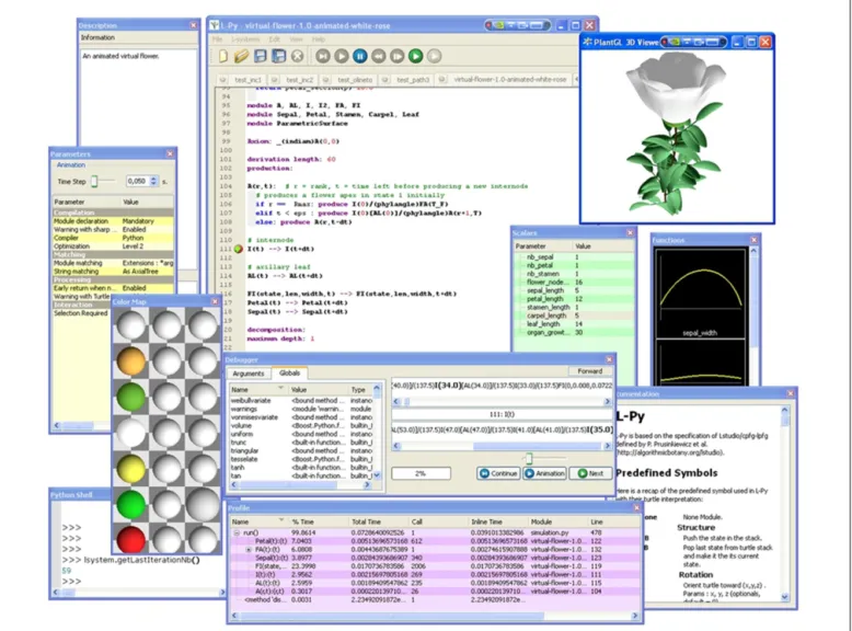
The L-Py IDE is also inspired by programming environments such as Visual Studio (Microsoft Corporation, 2011). Its config-urable interface using dockable panel widgets (see Figure 2) makes it possible to easily customize the working environment and its advanced development tools (profiler and debugger, etc.). The L-Py IDE incorporates two tools that help optimize models. First, a
debugger shows the user the successive rule applications that occur
during a derivation step with actual parameters and global variable values. The debugging can be constrained to detect the applica-tion of particular rules only. Second, a profiler provides the user with a detailed report of the time spent in each rule and function, and makes it possible to identify bottlenecks in the execution. The creation of these tools was facilitated by the introspection property of dynamic languages (introspection is the ability of a program to explore and possibly modify its own code). For instance, access at
runtime to the names and values of the different variables involved in a procedure is simple in a dynamic language and facilitates, for instance, the creation of the debugger.
L-Py as a component library: controlling L-systems execution from Python
L-Py has been developed as a C++ library embedded in Python that can thus be integrated into any Python-compatible appli-cation. For this, the L-Py library defines a number of structures (module, L-string, rule, L-system, etc.) that can be accessed from Python in an object-oriented manner. As a result, an L-system model can easily be manipulated by an external process. Such a process typically creates an L-system object, executes it for a num-ber of specified steps, possibly changes its parameters, resumes the execution, and finally gets the computed L-string. In this way, L-Py can be encapsulated as a simple component of a more com-plex modeling pipeline that integrates other components, possibly using formalisms different from L-systems.
The central issue of such an encapsulation strategy is to control the execution of L-Py models. An L-Py program contains global variables, functions, rules, and configuration/execution variables such as the number of derivation steps. From an external process, a user may want to access and change any of these elements. In L-Py, this can be done by using the Python/L-Py introspection mecha-nism or by using dedicated primitives implemented in L-Py. For instance, to explore a large parameter space for a given L-system, a user may want to vary parameters (e.g., global variables) of an L-system model after each execution. Such exploration cannot be made easily manually. The use of the introspection property of L-Py makes it possible to resolve this issue elegantly: a process that uses L-Py as a component can inquire about the internal variables of the L-Py model (global and configuration/execution variable) and directly access and modify them in memory. Global variables of the model become automatically and dynamically attributes of the L-system structure that contains the model, and can be modified as easily as any attribute of a Python object. Execution variables can also be modified with predefined L-Py functions. For example, to overwrite the axiom of an existing L-system object, an L-string can be built from a specified string of characters with the Lstring construct and then used to overwrite the contents of the L-system axiom. More generally, L-strings can be built from modules con-taining objects of any complex type as parameter values. Thanks to the dynamic typing of the language, parameters of any type can be introduced into the L-string and passed to an L-system. For example, the following program creates and runs iteratively Lsystem1using an increasing value of the global variable dr, incremented externally in each step.
Code2:
1 lsys = Lsystem(‘Lsystem1.lpy’) 2 print lsys.dr # This would print 0.02 3 axiom = Lstring(‘Apex(2)’,lsys) 4 for i in range(10): 5 lsys.dr += 0.02 6 lstring = lsys.derive(axiom,5) 7 interpretedstring = lsys.interpret(lstring) 8 scene = lsys.turtle_interpretation(interpretedstring) 9 Viewer.display(scene)
Line 1 reads in and creates an L-system structure from the Lsystem1code. The second line requests and prints the value
of the internal variable dr from the model lsys. Note that the global variables such as dr are automatically considered as attrib-utes of the L-system object. Line 3 creates an L-system string from a text string, using lsys module definition to interpret correctly the module names. This L-string will be used subsequently as the L-system axiom. Line 4 initiates a loop that will perform parame-ter space exploration for ten values of the dr parameparame-ter. At each iteration step, Line 5 changes the value of dr before performing 5 Lsystem derivation steps starting from the axiom (line 6) and assigns the resulting string to lstring. Note that in this case, only the production rules and the global variables of the L-system are used in the object, while the initial string (axiom) can be con-sidered as a variable (notion of L-system scheme,Herman and Rozenberg, 1975). The function derive can also be called with no argument and will use in this case the values of the axiom and the number of derivation to perform declared in the L-system. Finally, lines 7–9 interpret the resulting string geometrically using the turtle interpretation, and display the result in the viewer. These lines can also be summarized into one (more efficient) com-mand lsys.plot (lstring). However, they are given here to show that a user can finely control the execution of an L-system. Importantly, entire functions and productions of complex models can be changed similarly to the simple variable dr in the above example.
Creation and manipulation of an L-system object have also been encapsulated into OpenAlea (Pradal et al., 2008) as compu-tational nodes. Similarly to the example provided here, these nodes can be created with L-Py code and parameterized with a dictionary containing the names and new values of the variables. Examples of such use are given in Section “L-Py as Growth Component for Simulating an FSPM.”
The L-Py introspection mechanism: controlling L-system execution from L-Py programs
L-Py makes it also possible to control its execution, vari-ables, and rules from within L-Py models. For instance, the ExecutionContext object is accessible through the execContext() function and makes it possible to ask and modify the values of the L-Py model configuration/execution vari-ables. These variables control the number of derivation steps, the currently used group, etc. (a complete list is given in the online help; see also Standard L-Systems Features of L-Py in Appen-dix). After each iteration modelers also have access, through the EndEachfunction, to the resulting L-string and the correspond-ing scene graph. This enables global post-processcorrespond-ing of the mod-eled structure using regular Python code and external modules from within a model. In this way, an L-Py model can also act as an integrative framework for different modeling components (see for instance section “Minimizing Measurements in 3D Plant Architecture Reconstruction”). For example,
Lsystem3: 1 Axiom: A 2 production: 3 A--> B 4 B--> AB
produces a sequence of strings whose lengths follow the Fibonacci series. It can also be shown that the string produced in step t is the
concatenation of the strings produced in steps t-2 and t-1. Check-ing visually these properties with L-Py is easy and requires only adding two lines of code:
Lsystem3 (continued): 5 def EndEach(lstring):
6 print len(lstring), lstring
These lines print the length and the value of the current L-string and are called after each derivation step. The output exhibits the Fibonacci properties of the model:
Lsystem3 (output): 1 A 1 B 2 AB 3 BAB 5 ABBAB 8 BABABBAB
Modification to the string can be made in a similar way from within a L-Py model. Likewise, thanks to the dynamic language evalua-tion, it is possible to add or remove a rule during the execution of an L-system.
MODULAR L-SYSTEMS IN L-Py
Code modularity is the key to build complex and reusable mod-els. In our context, this raises the question of building reusable blocks based on L-systems that can subsequently be assembled. Modularity of the model may result from the decomposition of the structure into components such as internodes or leaves, which can be processed and defined independently (Hanan, 1992;Godin et al., 1998;Prusinkiewicz et al., 1999a) or from the decomposition of the model into of component aspects such as growth, photo-synthesis, and hormone transport (Cieslak et al., 2011). In this section, we discuss the support for decomposition into aspects, offered by L-Py.
One technique supporting such decomposition was proposed byFederl and Prusinkiewicz (2004), based on the concept of con-trolled derivations in L-systems. Different groups of production rules are identified by group Ids. Only one group is active in any derivation step. However, another group may be activated in the next derivation step, and so on. The selection of the appro-priate group can be conveniently made before each derivation step using the StartEach statement. Within a static language, however, parameters of the modules are declared at the begin-ning of the model and their declaration should take into account all parameters required for all groups. This limits the indepen-dence of the groups and thus the modularity of the composite L-system.
More recently,Cieslak et al. (2011)proposed another strategy to develop modular L-systems, based on the use of separate mod-ules to represent different aspects of the model. These modmod-ules can be combined such that one organ of the plant is represented by a list of modules, each reflecting a different aspect of the model. The rules related to the different aspects are described in different groups and are invoked sequentially. While this makes it possible to have separate definition of each group with their own modules and rules, a given element is modeled in this approach with several modules, which blurs its identity.
In L-Py, we elaborated on the approach of Federl and Prusinkiewicz (2004)and extended it with the use of a dynamic language to reinforce the decoupling of the different L-systems to assemble. The goal is to combine several independent L-systems, typically written by different persons, in different files (say for example files A.lpy, B.lpy, C.lpy). Each L-system can be considered as a processing unit dealing with an aspect of sim-ulation, for example substance transport, branch mechanics, or growth. An order may have to be respected in the application of the corresponding L-systems, as some of them may update L-string parameters subsequently used by other L-systems. We assume that the different L-systems operate on the same or closely related sets of plant components, e.g., apices, growth units, or internodes. As similar components in different L-systems may be identified by dif-ferent module names, a mapping between these names is defined in the third “translation” L-system. For instance, if the module representing an internode is named I in system A and S in L-system B, a rule I --> S will be created in the translation L-L-system A2B.Module parameters must also be translated. Detailed exam-ples of how this is done are given in Section “Managing L-System Modularity” in Appendix.
Different L-systems and their translations can be chained by the programmer to make up a unique compound L-system. To easily handle such chaining, a generic Python class ComposedLsystemis provided in L-Py. It takes two arguments: a list of L-systems to be chained (including translation schemes) and a list of interpretation schemes to be chained. A sketch of a typical code that must be defined to combine different L-systems follows.
Code4:
1 a,b,c = Lsystem(‘A.lpy’),Lsystem(‘B.lpy’), Lsystem(‘C.lpy’)
2 a2b, b2a, a2c = Lsystem(‘A2B.lpy’),Lsystem(‘B2A.lpy’), Lsystem(‘A2C.lpy’) 3 clsystem = ComposedLsystem([a,a2b,b,b2a],[a2c,c]) 4 lstring = clsystem.axiom 5 for i in xrange(K): 6 lstring = clsystem.derive(lstring) 7 clsystem.plot(lstring)
The first two lines create the different L-systems required for the model. The third line gathers them into a ComposedLsystem struc-ture. As arguments, two lists of L-systems are given. The first list contains the set of L-systems responsible for the production rules and the second list for the interpretation, given in the order in which they should be called. In the first list, the target L-system of the last translation (the “a” in b2a in the example below) must be identical to the first L-system of this list, while in the second list, the source L-system of the first translation (“a” in a2c) must be identical to the last L-system of the first list (i.e., “a” also). The next four lines simply run and plot the ComposedLsystem for a number K of iterations as if it were a simple L-system. In this case the chaining of L-systems is controlled by the ComposedLsystem primitive, but the modeler still has the possibility to write code that calls each Lsystem one after another a number of times (for instance to handle different time units in the different L-systems). This approach shows a great flexibility in assembling com-ponents by transforming L-strings expressed in the alphabet of
one L-system to that of another one. This approach may be com-bined with sub-Lsystems or other aspect-oriented approaches into a completely flexible and modular L-system framework.
MODELING PLANT GROWTH AT DIFFERENT SCALES IN L-Py The embedding of L-Py in a dynamic language has a number of consequences on the modeling possibilities themselves. Due to the non-strict typing system, connection with external modules and models is much simpler than with static languages. Here, we inves-tigate the consequences of this language specificity to key aspects of plant modeling.
SEAMLESSLY COMBINING L-SYSTEMS AND MTGs
In the late 1990s,Godin and Caraglio (1998)introduced a formal model called Multiscale Tree Graph (MTG) to represent a wide range of plant architectures, at varying scales of description, in a flexible and unified way. Since then, MTGs have been used widely to encode various types of plant architectures at varying scales (e.g.,Godin et al., 1999; Mündermann et al., 2005; Teobaldelli et al., 2008) and to analyze the resulting data with dedicated soft-ware such as AMAPmod (Godin and Guédon, 1997) and OpenAlea (Pradal et al., 2008). Today, in OpenAlea, MTG is the central data-structure that different modeling packages use as a standardized way to represent plants.
In order to exploit the large library of algorithms and mod-els built for MTGs in L-Py, we designed bidirectional translation and mapping mechanisms between L-strings and MTGs. Conver-sion between these structures is possible as they both represent a particular type of labeled tree graphs. L-strings represent axial tree graphs (Prusinkiewicz and Lindenmayer, 1990) while MTGs may integrate tree graph descriptions at several scales (Godin and Caraglio, 1998). Fortunately, it has been shown that, similarly to simple tree graphs, multiscale tree graphs can be encoded as strings (Godin et al., 1999). L-strings corresponding to MTGs can be defined using this property (Godin et al., 1999;Ferraro and Godin, 2000).
In brief, let us first consider an L-string representing the tree graph at the most microscopic scale of the MTG (e.g., at the scale of internodes I), of Figure 3 (left) e.g.,
I I I [I I] I...
where each I represent a plant module (here an internode), and opening brackets indicate branching points. Modules representing more macroscopic nodes of the MTG, corresponding for example to growth units U or to branching systems S, are inserted before the first microscopic module that composes them (Godin et al., 2005). The resulting string mixes modules at different scales. A small branching system S composed of growth unit U that can be decomposed as internodes I is thus encoded as:
S U I I I [U I I] U I...
This defines a multiscale L-string associated with the MTG (see Figure 3). For the L-Py interpreter to recognize that modules in the string belong to different scales, the user must explicitly asso-ciate each module type with a scale using the keyword “scale” in the module type declaration of the L-Py program:
FIGURE 3 | Comparison of MTG and an L-string. A branching system S is
composed of three growth units, which are in turn composed of two or three internodes. Left: a detailed representation of S at the scale of the internode. Middle: representation of the MTG on the top and the corresponding multiscale L-string on the bottom. Right: A geometric representation of the multiscale L-string.
module S: scale = 0 module U: scale = 1 module I: scale = 2
As in classical L-strings, modules in multiscale L-strings can have parameters of any type, including complex types and objects. The use of a dynamic language makes it possible to seamlessly con-vert L-strings into MTGs and, reciprocally, MTGs into L-strings. Indeed, in the conversion, L-string module parameters are auto-matically transformed into MTG node parameters (or vice versa) without the burden of duplicating parameters in memory or writing/reading data through exchange files.
Primitives to read/write and convert MTGs into L-strings (and reciprocally) have been designed and make it possible to manipulate MTGs directly within L-Py rules. These can be used for instance to initialize a simulation with a plant architecture measured experimentally:
Lsystem5:
1 from openalea.mtg import * 2 intialmtg = MTG(‘walnut.mtg’) 3 Axiom:
4 PlantFrame(intialmtg, scale = 3)
5 parameters = [’tipposition’,’bottomdiameter’, ’topdiameter’]
6 lstring = mtg2lstring(initialmtg,{‘S’: parameters, ‘U’: parameters, ‘V’: parameters})
7 sproduce(lstring) 8 interpretation: 9 S(tippos,bottomdiam,topdiam) --> _(bottomdiam) LineTo(tippos,topdiam) 10 U(tippos,bottomdiam,topdiam) --> _(bottomdiam) LineTo(tippos,topdiam) 11 V(tippos,bottomdiam,topdiam) --> _(bottomdiam) LineTo(tippos,topdiam)
Axiom is now defined as a rule (lines 3–7) that produces a string (line 7). The MTG of a measured walnut tree (Juglans regia L.;
Sinoquet et al., 1997) is first loaded (line 2, note that the func-tions for manipulating MTGs, such as MTG and PlantFrame used here, are independently provided by the MTG package of OpenAlea). This file contains the information related to the topol-ogy of the plant at three different scales (axis segments, axes, and plant). In addition, for some plant segments, it contains key information about their geometry, called “frame” informa-tion (this informainforma-tion was not systematically measured for all plant segments in the field). The frame information consists of the spatial location of the segment tip in a reference coordinate system originating at the basis of the plant, together with their bottom and top diameters. Based on the frame information avail-able for some segments in the MTG, the PlantFrame function makes it possible to compute the frame information for all the plant segments where it is missing, using predefined inference rules (Godin et al., 1999). As a result, the frame attributes (’tip position’,’bottomdiameter’,’topdiameter’) of the segments of the MTG are updated with the computed infor-mation. The MTG is then transformed into a multiscale L-string (lines 5–6), where the different modules corresponding to the plant segments (here labeled S, U, V) are given parameters corresponding to their frame information in the MTG. Finally, the sproduce statement of line 7 produces the multiscale L-string corresponding to the MTG (one can note the difference between produce and sproduce: produce creates a suc-cessor L-string from a list of modules, while sproduce creates a successor L-string from an already built L-string structure). The axiom defined by this string has thus been procedurally evaluated. Finally, to plot a graphical representation of the axiom, a simple interpretation rule is defined for each type of module (line 9–11) that uses the turtle to draw the complete plant structure by exploit-ing the frame data of the successive plant segments along the plant axes (Figure 9, left).
HIGH-LEVEL CONSTRUCTS FOR THE CONTROL OF TURTLE GEOMETRY As illustrated in the previous sections, the use of a dynamic lan-guage such as Python favors the openness of the modeling lanlan-guage (i.e., its ability to be extended) and its simplicity of use by pro-viding high-level constructs in the language. Both characteristics were considered as key guiding principles throughout the design of L-Py. In this section, we show how these principles were used to simplify the modeling of plant geometry by introducing new constructs to manipulate turtle geometry at high abstraction level.
Custom geometric primitives for plant representation at different scales
When representing plant architecture, most simulation systems use an explicit geometric representation of plant organs: intern-odes are represented by cylinders, leaves by small parametric surfaces, fruits by volumetric models, roots by generalized cylin-ders, etc. In recent years, however, abstract geometric models of plant organs have been introduced to represent plant architectures at more macroscopic scales in simulation models (e.g.,Cescatti, 1997;Boudon, 2004;Pradal et al., 2009;Livny et al., 2011). These approaches are based on the use of either volume or envelope models that represent groups of organs instead of individual organs. Such models can be readily designed in L-Py thanks to
the tight coupling with the PlantGL library (Pradal et al., 2009). A generic primitive, @g(geometry), allows the modeler to posi-tion any PlantGL model in space using the current turtle locaposi-tion and orientation. In this way, coarse geometric representations of plant architecture can be defined where parts of the tree crown are represented by parametric envelopes. The resulting architecture may then be used in conjunction with ecophysiological models that take a 3D scene as an input. Here we illustrate this possibility by computing the direct illumination of each crownlet in the plant using the Fractalysis library (Da Silva et al., 2008) from OpenAlea: Lsystem6:
1 from openalea.plantgl.all import AsymmetricHull 2 from openalea.fractalysis.ligth import
diffuseInterception
3 def EndEach(lstring,lscene):
4 lighting = diffuseInterception(lscene) 5 for id, light in lighting.iteritems(): 6 iflstring[id].name == ‘Crownlet’: 7 lstring[id].light = light 8
9 module Crownlet(height,radii,light) 10 production:
11 ... # generation of the tree containing Crownlet 12 interpretation:
13 Crownlet(height,radii,light)-->; (colormap(light)) @g(AsymmetricHull(height,radii))
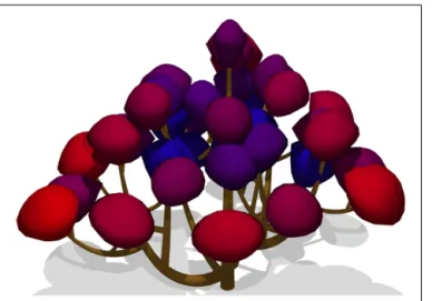
This L-system produces in each derivation step an L-string that is composed of modules Crownlet which are characterized by their height, maximum radii in four directions in the plane perpen-dicular to their main axis, and the total amount of light that they receive (defined in line 9). As explained in Section “The L-Py Intro-spection Mechanism: Controlling L-System Execution from L-Py Programs,” the L-string produced at each step and the correspond-ing L-scene can be post-processed in the EndEach function. The scene is a set of PlantGL objects that were derived from the L-string modules by the application of the interpretation rules (line 13). Each L-scene object thus contains an id corresponding to its associated module in the L-string (in L-Py, the L-scene ids sim-ply correspond to the position of their associated module in the L-string). In the EndEach function, the amount of diffuse light intercepted by every module of the plant is evaluated by a call to the Fractalysis library (line 4). The diffuseInterception primitive is passed a PlantGL scene and returns a dictionary con-taining pairs composed of module ids and of the amount of light intercepted by that module. To import this information back into the string, an iteration over the dictionary is made in lines 5–7. For each module id, the module name is checked (line 6) to select only crownlet modules and their light parameter is updated (line 7). Figure 4 shows a representation of the L-scene after construction of a tree made of a branching system bearing crownlets represented by asymmetric hulls and colored according to the total amount of light intercepted by each crownlet.
Seamless control of differential turtle geometry
In particular modeling situations, one needs to instruct the tur-tle to follow a predefined curve in 3D space. This is required for example when one wants to control the shape of a branch using a predefined template shape. For this, we assume that a curve of
length L is defined that represents the shape of a particular branch. In the 3D scene, at the position of the branch insertion on the par-ent branch, we then need to instruct the turtle to move along this curve from its current position. To achieve this,Prusinkiewicz et al. (2001)designed an algorithm to move the turtle in the 3D space based on differential geometry and using quantities such as local tangent, curvature, and step size. The following L-Py code gives a simple 2D version inspired from this algorithm.
Lsystem7: 1 length = 12.4 2 dl = 0.01 3 Axiom: FFF [+M(0)] FF 4 production: 5 M(l): 6 if l < length:
7 u, nextu = l/length, (l + dl)/length 8 tgt = curve.getTangent(u)
9 nexttgt = curve.getTangent(nextu)
10 rotangle = degrees(atan2(cross(tgt,nexttgt), dot(tgt,nexttg)))
11 produce +(rotangle) F(dl) M(l + dl)
The axiom defines a parent branch made of five segments and bearing a branch on the third one (line 3). The branch is produced by incremental application of rule M(i) until length length is reached (lines 5–6). First, normalized lin-ear abscissa of current and next points are computed (line 7), assuming that the turtle will make steps of constant size dl. This makes it possible to compute the angle by which the turtle should turn (lines 8–10) according to the reorien-tation of the tangent between these points before making the move (line 11). The recursive application of this rule produces the branch shape as specified by the PlantGL Curve2D object curve, defined elsewhere either graphically or procedurally (see section “A Complete Integrated Development Environment” and Figure 5B).
However, one can note that the corresponding code contains low-level instructions related to the computation of the local
FIGURE 4 | Representation of a tree at the scale of crownlet using of the asymmetric hull primitive of PlantGL and with light interception computation using Fractalysis (Da Silva et al., 2008).
curvature on the template curve (lines 7–10). This may obscure the overall code with instructions related to differential geom-etry management, which are not essential to the expression of the model itself. To alleviate this difficulty, we abstracted this differential geometry management by introducing the primitive SetGuide(curve,length), which instructs the turtle to fol-low the given curve until the total length of its moves reaches the prescribed value length. The algorithm used to control the turtle frame movement from the curve definition is inspired from
Bloomenthal (1990)to control branch shape in a global to local manner (details of the SetGuide primitive are depicted in section “The SetGuide Primitive” in Appendix). Using this primitive, we can define the shape of a branch and keep clear the main L-system code:
Lsystem8:
1 Axiom: FFF [&(90) SetGuide(curve,length) M(0)] FF 2 production:
3 M(l):
4 if l < length:
5 produce F(dl) M(l + dl)
In the axiom (line 1), as soon as the turtle has been rotated to draw the branch, it is instructed to follow the curvature specified by the template curve curve (SetGuide primitive). The turtle is moved recursively forward following at each step the bends defined by curve, leading to the result depicted in Figure 5B. Note that if the SetGuide primitive is removed, the code is still valid L-Py code, where the turtle goes straight instead of following any curved trajectory (Figure 5A). In fact, SetGuide made it possible to completely separate the spec-ification of the branch geometry from the specspec-ification of the topology.
This design pattern can be applied to a more complex branch-ing system to control the shape of branches in a global to local manner. The following code illustrates the use of SetGuide to control the bending of a complete branching system recursively with a unique template curve.
FIGURE 5 | Construction of the geometry without (A) and with (B) the SetGuide primitive. It takes as input a user-defined template curve
Lsystem9: 1 Axiom: M(0,0) 2 production: 3 M(l,order):
4 if order < MAXORDER and l < length:
5 produce F(dl) iRoll(phi)[ˆ(60)SetGuide(curve, length-l)M(l,order+1)]M(l+dl, order) 6 else: produce
The apex M now has an additional parameter “order” to con-trol the order of the branch. Apices whose order is greater than MAXORDERabort (line 4). The apex of order 0 is not prefixed by any SetGuide (line 1) and thus assumes a Euclidean space and develops a straight vertical trunk. By contrast, the branches built by lateral apices at order 1 and 2 are all prefixed by a SetGuide (line 5) and will then follow the specified template curve curve for the remaining length length-l. The resulting branching structure is illustrated in Figure 6.
Modeling shape variation
Plants architectures frequently show gradients in the shape of their organs. At different scales smooth variations of form and ori-entation may be observed: in petal shapes in flowers, in branch bending along a trunk, or in crownlet shapes and volumes in a tree crown (e.g.,Bell, 1991;Barthélémy and Caraglio, 2007). Continuous variations in shapes may also arise throughout time due to growth and aging: leaves may unfold out of the bud for instance or fold due to a change in their water status, branches may change their shape due to interaction between gravity and growth, while trees may undergo deep shape metamorphosis throughout their lifespan (Hallé, 1978). Common to all these processes is the notion that a shape changes seamlessly (or “continuously”) either in space or in time. Describing such changes is critical in models of plant architecture. In the context of L-systems, the importance of this phenomenon was recognized byPrusinkiewicz et al. (2001)who proposed to model attributes of plant architec-ture as functions of their location along the main axis (positional information).
Here again, the tight coupling between L-Py and PlantGL provides a powerful solution to address this issue. The ProfileInterpolationobject of PlantGL makes it possible
FIGURE 6 | Left: simple recursive structure with straight branches, Right: use of a template curve shown in the inset to define branch geometry. S-shaped branches produce a more realistic appearance and can
be easily specified in L-Py.
to smoothly interpolate between user-defined curves. The user specifies a set of keyframe curves at given index values. Then the ProfileInterpolationuses an interpolation scheme (e.g., the BSpline interpolation scheme;Piegl and Tiller, 1997) to com-pute intermediate curve values for any index between the extreme index values.
This function can be used for instance in combination with SetGuide to control the shape of axes in a branching system in a high-level manner. Using positional information (Prusinkiewicz et al., 2001) and ProfileInterpolation, we can compute for every position on the trunk of the plant a branch shape defined as a smoothly interpolated value between user-defined curves at different key altitudes on the trunk.
Let us modify for instance the previous L-system to control the shape of branches on the trunk according to a gradient of template curves. Lsystem10: 1 axisfunc = ProfileInterpolation([axis1,axis2,axis3], index = [0,0.6,1],degree = 2) 2 Axiom: M(0,0) 3 production: 4 M(l,order):
5 if order < MAXORDER and l < length:
6 produce F(dl) iRollR(phyllotaxy)[ˆ(60) SetGuide (axisfunc(l/length),length-l) M(l,order+1)] M(l + dl, order)
7 else: produce
An interpolation scheme, using these reference curves is set up by specifying the normalized indexes corresponding to these curves, and the degree of interpolation (line 1). Then the SetGuide is set up to move on the axis curve defined for the normalized index l/lengthby the interpolation scheme. Figure 7 illustrates the result of this scheme applied to different sets of key curves.
This interpolation procedure can also be used to animate plant development in a flexible manner as illustrated by the example code below (Figure 8).
Lsystem11: 1 axisfunc = ProfileInterpolation([axis1,...,axis4], times = [0,0.25,0.5,0.75,1],degree = 3) 2 length, dl, dt = 10, 1, 0.01 # constants 3 Axiom: Leaf(0,length) 4 production: 5 Leaf(t,l) --> Leaf (t+dt,l) 6 interpretation:
7 Leaf (t,l)--> Sweep(axisfunc(t), profile,l, dl,leafwidth)
FIGURE 7 | Examples of structures whose branches shapes are defined as interpolation of three curves (shown on the right of each tree).
Lengths of lateral branches are also dependant of the position of the branches on the trunk and is controlled with an extra graphical function.
FIGURE 8 | Animating a rolling leaf (bottom) using graphically specified curves and functions (top). The first curve specifies the cross section of the leaf,
the second specifies leaf width along the main axis of the leaf, and the remaining four curves specify the key shapes of the main axis of the leaf over time.
A sequence of keyframe curves defining the midrib of a leaf gradually rolling down were defined graphically by the user (Figure 8, top right). An interpolation scheme is set up using these reference curves by specifying their time points and the degree of interpolation (line 1). The L-system production sim-ply advances the “age” t of a module representing the leaf (line 5). Each application of this production is followed by an inter-pretation step (line 7). The produce statement in line 7 creates the leaf blade geometry. The leaf midrib is specified by the L-Py built-in Sweep primitive that corresponds to an extension of generalized cylinders (Bloomenthal, 1985) to arbitrary contours, including non-closed contours. This primitive is itself defined on the basis of the SetGuide primitive. In the example code, the contour is specified by the SetSection primitive and defines the transversal section of the leaf blade. The axis of this general cylinder is defined as the interpolated curve at time point t. The resulting sample frames of the animation are depicted on Figure 8. EXAMPLE OF FSPM APPLICATIONS IN L-Py
In this section, we show how L-Py can be used to create complex FSPM scenarios. A first example illustrates how advanced analysis tools can be used to parameterize a L-system that reconstructs trees from observed data. The second example illustrates how modu-larity can be used to decompose an existing FSPM into reusable components. A last example reports the use of L-Py as a training tool for high school students to reconstruct a virtual ecosystem.
MINIMIZING MEASUREMENTS IN 3D PLANT ARCHITECTURE RECONSTRUCTION
The compatibility between L-Py and MTGs opens powerful new possibilities to manipulate plant simulations. Let us consider for example the problem of digitizing complex tree architectures. Dif-ferent techniques to address this problem have been proposed in the literature and only manual techniques, such as magnetic 3D digitizing (Sinoquet et al., 1997), can currently precisely record both the 3D spatial coordinates and the topological structure of a plant in terms of annual shoots or growth units. Unfortunately, manual digitizing techniques are extremely time consuming and methods to simplify them are much needed. An intuitive idea is to exploit the redundancy of tree structures and only digitize the main branches of the tree. Smaller branchlets, which are highly repeti-tive, are then generated procedurally. Assuming that such a scheme
has been implemented, the question is how to assess the resulting semi-automatic reconstruction method. The seamless combina-tion of plant architecture simulacombina-tion and analysis provided in L-Py makes it possible to simply address this issue.
Let us illustrate how such an approach would be implemented using L-Py. We assume that a reference plant has been digitized. Here, for sake of simplicity, we reuse the digitized walnut tree introduced previously. We also assume that a simple L-Py proba-bilistic model has been designed to generate small branches from bud modules. We want to assess the ability of this model to recon-struct faithfully the digitized small branches of the tree, and thus to avoid the overhead of digitizing small branches in similar trees. For this, we first remove the small branching systems from the digitized tree. Modules of the digitized tree have three different types: modules of type V (resp. U) represent growth unit segments from the last year (resp. from the second last year). All other mod-ules are of type S and represent branch segments from previous years (Figure 9, left). In our example, we chose to remove the branching systems made up by growth units from the last 2 years, i.e., of type V and U. This can be done by defining a simple L-Py rule in the previous L-system file (lsystem5.lpy) that replaces every branching system starting with a U and following a segment S by a bud:
Lsystem5 (sequel): 1 production:
2 S(tip0,dbot0, dtop0) < U(tip,dbot,dtop) --> Bud%
This rule removes in a single derivation step all the branch extrem-ities starting with a U from the multiscale L-string representing the digitized plant and replaces them by Bud modules (Figure 9, right). In a subsequent derivation step, the bud modules are then used to produce new branching systems using a probabilistic model. This model is defined by an L-Py rule:
Lsystem12: 1 production: 1 Bud:
2 nbelem = gauss(AVG_NBELEM,STDEV_NBELEM) # Gaussian distribution
3 for i in xrange(nbelem):
4 nproduce U # generates the growth units of the main axis
5 ramif = random()
(with fixed probability)
7 nproduce [V]
8 nproduce V
This rule specifies that a bud is replaced by a shoot made of a ran-domly chosen number of segments U that can each bear (or not) a segment V and that terminate by a segment V. Note that we omit-ted to show the computation of the branch geometry to keep the example simple. As a result, all the removed digitized branches are replaced by artificially generated small branches, thus providing a partially digitized and partially simulated tree.
Then, to assess the quality of the resulting semi-simulated tree, we make use of the plant structural comparison primitive avail-able in the VPlants package of OpenAlea (Ferraro and Godin, 2000). This function compares the structures of two plants (here the digitized and semi-simulated trees) and returns a list of pairs
FIGURE 9 | Use of a digitized 20-year-old walnut tree (Juglans regia L.) as the axiom of a simulation. Right, shoots produced during the last
2 years are removed. Simulation process will use this structure as new axiom and produce algorithmically new shoots. Generated shoots will be compared with measured ones. Bottom, a detail view of the process: from top to bottom, original branching system, pruned system with insertion of Bud represented as red sphere, and example of regenerated structure.
of plant segments from both plants that were found to match each other. The more matching segments are found in both trees, the better the reconstruction. The normalized length of the returned list, Q= 2 × L/(L1+ L2), L being the size of the returned list and
L1 and L2respectively the sizes of the compared trees, can thus be used as an indicator of the faithfulness of the model. If Q is greater than a specified threshold, the simulated tree is considered as a faithful reconstruction and the list contains pairs referring to most of the components of both plants. In the opposite case, the list is close to being empty and the reconstruction is considered poor. The following function illustrates how such a comparison can be carried out in L-Py:
Code13:
1 from openalea.treematching import * 2 def compare(lstring, initialmtg): 3 reconsmtg = lstring2mtg(lstring) 4 m = Matching(reconsmtg,initialmtg)
5 return 2 * len(m.getMatchingList())/(len(reconsmtg)+ len(initialmtg))
The compare function takes as arguments the current L-string representing the reconstructed plant and an MTG representing the initial digitized tree. It first transforms the L-string into an MTG and then compares the two MTG structures using a primitive from the treematching module of OpenAlea. As a result, it returns the estimated value of Q for this comparison.
This function can then be used to explore the parameter space of the probabilistic branching model (here through varying the branching probability) so as to find those parameters that make it possible to reconstruct trees faithfully with respect to the original digitized tree. This is done in the following function that assembles the different components of this pipeline:
Code13 (sequel):
6 def optimize_reconstruction (minv,maxv,vstep): 7 l = Lsystem(‘lsystem5.lpy’)
FIGURE 10 | Result of the comparison between regenerated structures and the measured one. The scores of the different branching systems are
given by the colored curves and the average value by the black curve. Maximum average score is reached with a probability of 0.77 and gives a score of 0.8.
8 initialmtg = l.initialmtg 9 prunedstring = l.derive() 10 Q = zeros((maxv-minv)/vstep)
11 for i, branchingprob in enumerate (arange(minv, maxv,vstep)): 12 l = Lsystem(‘lsystem12.lpy’) 13 l.BRANCHINGPROB = branchingprob 14 lstring = l.derive(prunedstring,1) 15 Q[i] = compare(lstring,initialmtg) 16 plot(arange(minv,maxv,vstep),Q)
In our example, Q varies non-monotonically between 0.65 and 0.85 when varying the probability parameter between 0 and 1 (see Figure 10), showing that best reconstructions are reached for a branching probability close to 0.77 in our stochastic model. Three examples of evaluated reconstruction are given in Figure 11 with branching probability of 0.4, 0.6, and 0.77 respectively. Red color represents parts of the structure whose Q coefficient is greater than 0.8.
L-Py AS GROWTH COMPONENT FOR SIMULATING AN FSPM
We now illustrate the use of the above modular approach on a real complex FSPM, MAppleT, simulating the growth of an apple tree (Costes et al., 2008) and originally developed using
L-studio/lpfg. This model mixes stochastic topological construction
with a bio-mechanical model for the geometry (see Figure 12). Thanks to syntax compatibility between L-Py and L+ C, the code port mainly consisted in translating and simplifying the C++ instructions into Python. Additionally, scientific tools from Python and OpenAlea were readily accessible from within the model (for instance, 2D plot with Matplotlib).
An L-system model, such as MAppleT, is composed of sev-eral processes that simulate the growth and internal processes of a plant. In the original model, groups of rules were defined to model different processes: (a) updating state of organs accord-ing to a calendar (bud break, floweraccord-ing, etc.), (b) computa-tion of growth units lateral produccomputa-tions according to stochastic
FIGURE 11 | Comparison between regenerated structure and measured one. Reconstructions showed here are built with ramification probability of
0.4, 0.6, and 0.8 respectively. The six main branching systems of the tree are
compared to the original ones using a structural comparison method (Ferraro and Godin, 2000). Red and blue color means that structural difference is more or less than 20% respectively.
models, (c) growth process, (d) biomechanics. During refactor-ing, the code was divided into distinct L-systems correspond-ing to these different groups of rule to achieve modularity. Because they came from a single original L-system code, these L-systems components used similar module naming convention and thus were readily compatible with each other (see Modular L-Systems in L-Py). The parameters of the modules were stored in a generic container object whose contents can be updated by each system component. Parameters used by different L-system components were given a unique name in all of these. For instance, the growth process component (c) requires infor-mation on the number and types of components to create at each time step. This information is provided by the stochastic process component (b) using a consistent naming convention in both components.
Usually the different processes also rely on a number of global variables. To change their values, a dictionary containing the
names and values of global variables can be passed to the L-systems and can be applied using the introspection mechanism presented in Section “L-Py as a Component Library: Controlling L-Systems Execution from Python.” In this way, the global variables can be passed from one process to the next one. Each process can thus update these settings to inform the other processes if needed.
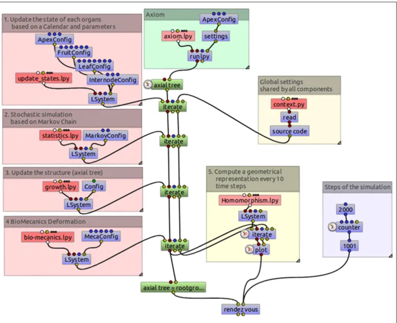
To better demonstrate the modularity of the code resulting from this decomposition of MAppleT, the L-system compo-nents were assembled graphically using a dataflow in OpenAlea (Figure 13). As opposed to code representation, dataflows give a visual representation of the logical dependency structure of the FSPM. The composition of the components can be made graphi-cally by the modeler by linking input and output of the different L-systems components and making it possible for the system to pass on the L-string and the dictionary of global parameters. The resulting graph (dataflow) can be executed and runs the pipeline throughout.
FIGURE 13 | Data flow of the MAppleT simulation. The model has been decomposed into several independent processes that can be combined and
Thanks to this modular decomposition, interesting manipula-tion of the assembled models can be made. For example, the user has the possibility to enable/disable some of them upon request. Figure 12 right illustrates for example the result of the model in which the Biomechanics component has been disabled.
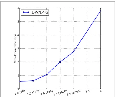
Based on this implementation of a real-size FSPM, we could carry out a comparative analysis of the computational perfor-mances of L-Py and that of static language implementations. L-Py was able to generate an entire architecture (10,000 components generated over 4 years) in reasonable time (5–10 min). In gen-eral, simulation with L-Py can be faster than with lpfg for small models (since it avoids compilation), but is five to six time slower than lpfg for more complex models of a 4-year-old apple tree (see
FIGURE 14 | Computation time comparison with between L-Py and
lpfg for MAppleT. The horizontal axis represents age of the simulated tree with estimated number of elements of the tree.
Figure 14). This is due to Python code interpretation of rules which is relatively slow compared to a compiled language like C or C++ (Prechelt, 2000). However, the L-Py interpreter written in C++ maintains acceptable performances.
L-Py AS A TRAINING TOOL FOR THE CLASSROOM
During French school year 2009–2010, we tested the use of L-Py as a tool for teaching scientific method in the context of a multi-disciplinary class on botany and computer science at high-school level (15- to 16-years-old pupils, 3 h per week during 35 weeks). The program of the class included both botanical and computer science/mathematics courses. The aim of the class was to reconstruct in 3D the vegetal structure of a 10 m× 10 m plot of plants typical from the local flora. The pupils measured the plants in the field, made diagrams and drawings of the plant architectures (see Figure 15), and registered the spatial distribution of observed plants. In the classroom, they were working hands on the computer and using L-Py as a modeling platform. They first learnt how to generate simple fractal and plant structures. They could create soon first simple models of plant structures. Then, using more sophisticated and generic models prepared for the occasion, they easily used their knowledge of L-Py to extend and customize these models according to the measured plants. Modifications ranged from simple parameter modification to addition of new rules in the L-systems. A number of individual plant models were thus designed by different groups of pupils in L-Py and were assembled into a single scene according to the measured distribution. Finally the scene was exported and rendered withBlender (2011)and a film corresponding to a virtual exploration of the 3D scene was produced. This experience gave us important feedback on L-Py during its testing phase. It first showed that the software can be used with success for training students in a multi-disciplinary con-text. L-Py turned out to be robust enough to support intensive use (and misuse) by pupils. The feedback from the classroom led us to adapt L-Py in various ways: simplify the visual interface, intro-duce debugging tools, and design new language features (such as the SetGuide and the curve interpolation primitives).
FIGURE 15 | Illustration of an application of L-Py in teaching. Students were in the field to map some botanical drawing of Euphorbia. Some virtual models