Endogenous structural change and climate targets.
Texte intégral
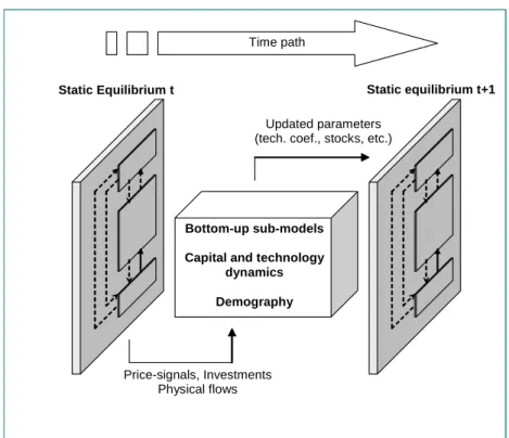
Figure
Documents relatifs
Abstract: We investigate the economic impact of stochastic endogenous extreme events and insurance in a growth model. Our analytical results and computational experiments show that
Key Words: climate change concern; wealth; control; country wealth; household wealth..
Results suggest that (i) it is feasible to perform event attribution using transient simulations and nonstationary statistics, even for a single model; (ii) the use of
Results suggest that (i) it is feasible to per- form event attribution using transient simulations and non-stationary statis- tics, even for a single model, (ii) the use of
Habitat suitability change is shown for three future change scenarios (BAMBU, GRAS, and SEDG) and for three model types (Climate-only [a –c, j–l], Dynamic LULC [d–f, m–o], and
To investigate the impact of early neutrophil recruitment on the control of infection we used C57BL/6 mice depleted of neutrophils during the first three days of infection using
The Green Climate Fund could test innovative approaches to the integration of adaptation and mitigation and stimulate changes at the national level in recipient countries and at
Other papers of this special issue cover various subjects: the retrieval algorithms (Kyr¨ol¨a et al., 2010a), the data characterization and error estimation (Tamminen et al., 2010),
