A tale of two diversities

HAL Id: hal-02090938

https://hal.archives-ouvertes.fr/hal-02090938

Submitted on 9 May 2019

HAL is a multi-disciplinary open access

archive for the deposit and dissemination of

sci-entific research documents, whether they are

pub-lished or not. The documents may come from

teaching and research institutions in France or

abroad, or from public or private research centers.

L’archive ouverte pluridisciplinaire HAL, est

destinée au dépôt et à la diffusion de documents

scientifiques de niveau recherche, publiés ou non,

émanant des établissements d’enseignement et de

recherche français ou étrangers, des laboratoires

publics ou privés.

A tale of two diversities

Pierre Courtois, Charles Figuieres, Chloe Mulier

To cite this version:

Pierre Courtois, Charles Figuieres, Chloe Mulier. A tale of two diversities. Ecological Economics,

Elsevier, 2019, 159, pp.133–147. �10.1016/j.ecolecon.2018.12.027�. �hal-02090938�

A Tale of Two Diversities

Pierre Courtois

_{, Charles Figuières}

_{, Chloe Mulier}

b _{Aix-Marseille Univ., CNRS, EHESS, Centrale Marseille, AMSE, Marseilles, France} c _{Innovation, Montpellier Univ., CIRAD, INRA, SupAgro, France}

Keywords:

Biodiversity indices, Conservation management strategy, Ecological interactions, Public policy, Species prioritization criteria JEL Classification: C6, Q5

Abstract:

Efficient biodiversity management strategies aim to allocate conservation efforts so as to maximize diversity in ecological systems. Toward this end, defining a diversity criterion is an important but challenging task, as several different indices can be used as biodiversity measures. This paper elicits and compares two criteria for biodi-versity conservation based on indices stemming from different disciplines: Weitzman's index in economics and Rao's index in ecology. These indices use different approaches to combine information about measures of (1) the probability distributions of the species that are present in an ecosystem (i.e. survival probabilities) and (2) the degree of dissimilarity between these species. As an important step toward in situ conservation criteria, we add to these elements information about (3) the ecological interactions that take place between species. Considering a simple three-species ecosystem, we show that criterion choice has palpable policy implications, as it can sometimes lead to divergent management recommendations. We disentangle the roles played by elements (1),(2) and (3) in the ranking of outcomes, which allows us to highlight several specificities of the two criteria. An important result is that, other things being equal, Weitzman's in situ ranking tends to favor robust species that are least concerned with extinction, while Rao's in situ ranking generally gives priority to more vulnerable species that are closer to extinction.

1. Introduction

The way in which resources should be allocated to manage threa-tened species remains a controversial issue. Conservation budgets are limited and management priorities must be set. An illustrative example of one such controversial conservation expense is the Australian cam-paign to rescue the last few specimens of Christmas Island pipistrelle,

Pipistrellus murrayi. Between 2004 and 2009, more than 276,000$ was

spent to support habitat corridors for the species.1_{Despite these efforts,}

the campaign failed and the Christmas Island pipistrelle has since gone extinct. The plight of this species has prompted an uncomfortable question: should the rescue campaign have taken place at all? In the current context of massive species extinction (e.g.Ceballos et al., 2017), an increasing number of scientists argue that the diversity and robust-ness of ecosystems can best be maintained by focusing management efforts on ensuring that species don’t become threatened in the first place rather than on tackling lost causes.2 _{Identifying the precise}

objective(s) of conservation policy is at the crux of this issue. The science of biodiversity conservation has grown rapidly in recent decades, in particular, on two related fronts. First, further reflection has advanced the definitions and measures of biodiversity, producing what could be called a “biodiversity index theory ”(for general overviews, see

Baumgärtner, 2004a,b; Magurran, 2004; Eppink and van den Bergh, 2007). Building on this first front, progress has also been made re-garding how to maximize a biodiversity measure, or more generally a biodiversity-related goal, subject to a number of constraints. The challenge here is to understand the nature of a “prioritization solution ”(e.g. the extreme policy inWeitzman’s,1998Noah's Ark metaphor). It is also to make this solution operational for in situ conservation policies.

In situ, species interact and as extinction is partly due to these

inter-actions, progress has been made to take species interrelations into ac-count when designing conservation criteria (Witting et al., 2000; Baumgärtner, 2004a; Simianer, 2008; Van der Heide et al., 2005;

Courtois et al., 2014).3_{As a result, at least at the conceptual level, we} *_{Corresponding author.}

E-mail addresses:pierre.courtois@inra.fr(P. Courtois),Charles.Figuieres@univ-amu.fr(C. Figuières),mulier@supagro.fr(C. Mulier). 1_{Seehttps://www.environment.gov.au/.}

2_{Regarding species prioritization and related debates about conservation choices, the reader may refer toWilson et al. (2011), Joseph et al. (2011), Carwardine}

et al. (2012), Schultz et al. (2013), Courtois et al. (2014, 2018), Bennett et al. (2014), Frew et al. (2016), Gerber (2016), or Lacona et al. (2017), among others. 3 _{Note that in situ is also referred to in the wild in the literature, cf. IUCN.}

2. A Class of in situ Prioritization Problems

Consider an ecosystem with N species. Each species i, i = 1,…,N, is characterized by a survival probability Pidefined as the probability that

species i does not got extinct over a given time period.7_{Assume that}

survival probability depends on demographic and genetic properties of species i, on abiotic factors, on the conservation effort it receives, and, as a result of ecological interactions, on the survival probabilities of the two other species Pj, with j≠i. We denote by xithe protection effort of

species i and consider xi {0, ¯}x, meaning that a species is protected

( = >xi x¯ 0) or not (xi= 0). We further assume that the simultaneous

protection of more than one species is not affordable, i.e. the entire available budget is just enough to cover the protection of a single species.8_{Without being too specific for the moment, if X stands for a}

N-dimensional vector of efforts, with components xi, and P is the vector of

linearly interdependent survival probabilities, with components Pi, the

link between efforts and probabilities is a N-dimensional vector of functionsPsuch thatP= P( )X .

We compare protection plans on the basis of how well they perform as measured by indices of expected diversity. We use two alternative indices: Weitzman's index, noted W(P), and Rao's index, R(P). Both belong to the family of expected diversity measures that aggregate dissimilarities between species. They combine, albeit in different ways, measures of, i) species' probability distribution, and ii) species' dissim-ilarity. Here, the probability measure considered is the survival prob-ability of species. Given the link between interdependent probabilities and efforts, P X( ), we can construct in situ expected diversity indices,

W( )X W(P( ))X , and R( )X R(P( ))X . Under this framework, the present paper makes an original contribution to the literature by ex-ploring and comparing optimal in situ protection plans. We accomplish this by solving the programsmaxXW X( )andmaxXR X( )and compare

their respective outcomes.

Next we address the details of P, X,W and R.

2.1. Interdependent Survival Probabilities

We assume each species i has an autonomous survival probability we denote qi∈[0,1[,i = 1,…,N. This probability can be evaluated on the

basis of demographic and genetic properties of species (i.e. reproductive capacities, genetic erosion, [ …]) as well as on abiotic factors impacting species survival such as geographic range and habitat breadth — ex-amples of which can be found inGandini et al. (2004), Alderson(2003, 2010) or Verrier et al. (2015). We assume that near 0 autonomous survival probability means that the species is fragile and likely to be

threatened while close to 1 autonomous survival probability means the

species is robust and a priori least concerned by extinction. Principal feature of autonomous survival probability – and this explains the qualification autonomous – is that it ignores the impact of species

4_{On a practical level,Joseph et al. (2008)applied Weitzman's prioritization} approach to assess New Zealand conservation allocation. Variants have been used byMcCarthy et al. (2008)to allocate surveillance effort over space for preventing biological invasions.

5_{A range of other important papers on the topic includesWeikard et al.}

(2006), Ricotta (2004), Sarkar (2006), Whittaker et al. (2005), Bossert et al. (2003), Crozier (1992) and Faith (1992).

6_{As we explain later, although a two-species ecosystem would be even} sim-pler, it would not allow us to study the role of dissimilarities on optimization outcomes. At least three species are needed for that purpose.

7_{Note that survival probability is fully related to extinction probability but} may well covary with rarity. Although extinction occurs when all the popula-tions of a taxon decline to zero, rarity does not consistently lead to high ex-tinction risk (Harnik et al., 2012). First because species may be rare because they have small geographic ranges, narrow habitat tolerances, small popula-tions or any combination thereof. Second because high abundance and fe-cundity do not consistently lead to low extinction risk (Dulvy et al., 2005). It follows that survival probability here, is neither a measure of abundance nor of species frequency. Instead, it can be assessed on the basis of the several ex-tinction probability criteria provided by the literature, see for instancehttp:// www.iucnredlist.org.

8_{Note that we assume therefore that marginal cost of effort is symmetric.} Assuming a conservation budget B, a symmetric marginal cost c and a linear budget constraint, we have =x¯ B c/ . Symmetry assumption could simply be released by assumingx¯i=B c/ibut it will add unnecessary complexity to our

model. Interested readers may refer toCourtois et al. (2018)for a detailed discussion on the impact of cost asymmetry in this class of modelling problems.

possess the means to rationalize in situ conservation efforts.4 _More

specifically, t he p roblem w e f ace i s a c hoice b etween m eans, a s the biodiversity index theory does not identify a unique, “superior” index of biodiversity. Rather, it offers a r ange o f m eaningful i ndices, which, when used as objective functions in optimization problems, may lead to different solutions. A key question to address is what is the conservation philosophy underlying these indices? By grounding conservation policy on one index rather than another, what weight is given to extinction probabilities, attribute dissimilarities and the role of species in the network of interactions?

Answering this question requires comparing the outcomes of in situ optimization exercises that use different b iodiversity i ndices a s the objective function to be maximized. An important sub-class of indices is based on data about dissimilarities between species (Rao, 1982, 1986; Weitzman, 1992, 1998; Solow et al., 1993; Hill, 2001)5_{. Gerber (2011)}

provides an axiomatic comparison of the last four indices, though not in a context of in situ protection plans and therefore, omitting the fact that species' survivals are interrelated. Rao's index was not included in this comparison, despite its importance in ecology and biology. However, the mathematical properties of quadratic entropy have been extensively studied in Champely and Chessel (2002), Pavoine et al. (2005), Rao (2010), Ricotta and Marignani (2007), Ricotta and Szeidl (2006) and Shimatani (2001).

The present paper makes an original contribution by examining the consequences of considering two alternative diversity indices as the objective function to be maximized in a prioritization framework:

Weitzman ’s ( 1992, 1998) index, which is popular in several literatures including economics, and Rao ’s ( 1982) index, which is used mostly in ecology and biology, but largely ignored by economists. Both indices simultaneously account for species distribution probability and dis-similarity measures. The axiomatic properties of both indices have been elicited (Rao, 1986 ; Bossert et al., 2003), which gives them some transparency as measures of diversity.

Since our goal is to understand basics of protection policies, we simplify the analysis whenever possible. Simplifications c oncern the ecosystems studied as well as protection policies. We focus on a three-species ecosystem6 _{with ecological interactions. Weitzman's and Rao's}

criteria are used for the comparison of particularly simple preservation policies, in which the decision maker (e.g. a national park manager) has only enough funding to address the management of a single species. In this situation, he must decide which species should be allocated con-servation funds. Should he make this decision based on, for example, the direct benefits t hat s pecies p rovide, o r t he i ndirect b enefits for-warded via ecological interactions?

The paper proceeds as follows. In Section 2, we model the two in situ prioritization criteria. After describing the characteristics of our three species ecosystem, we define how both indices combine different pieces of information and explain how prioritization criteria are derived from indices. Section 3 aims at disentangling the role of each of the elements embedded in the different c riteria, n amely ( i) a utonomous survival probabilities, (ii) dissimilarities, and (iii) coefficients of ecological in-teractions. General insights are raised on how the two criteria value these three pieces of information. We conclude the paper with a dis-cussion on the limits of the approach and some perspectives regarding future work on the topic.

= … Pi [ , ¯],P Pi i i 1, ,N < r | |ij 1 = + + Pi qi xi r P q [0, 1[ , x {0, ¯},x j i ij j i i (1) meaning that interdependent survival probability Piis the autonomous

survival probability qiof species i plus the variation of this probability

due to conservation efforts xi and the marginal impact rijany other

species j has on the survival probability of species i, this impact being possibly positive as negative according to the biotic relationship.

In order to formally define the system of interdependent survival probability describing our N species ecosystem, we define:

… … … … … q q q r r r r r r P P P P P P P P P x x x x x x Q R P P P X X , 0 0 0 , ¯ ¯ ¯ , , , ¯ ¯ ¯ . N N N N N N N N N N 1 2 12 1 21 2 1 2 1 2 ¯ 1 2 1 2 1 2 ¯ 1 2

In matrix form, the system of interdependent survival probabilities reads as:

= + +

P Q X RP, (2)

and under the condition that matrix IN_{−R is invertible, with I}N_the

(N × N) identity matrix, the system Eq. (2) can be solved to give:

= +

P [I R] *(1 Q X). ₍₃₎

Note that this condition is not particularly demanding here as it translates in a very specific relationship between marginal impact parameters. To illustrate it, in the three species case, this condition is not met iff r23r32+ r12r21+ r13r31+ r12r31r23+ r21r13r32= 1, i.e. a

very specific equality that has no reason to be true.

We deduce that a particular protection plan X induces a particular vector of survival probabilities, withP P( )X [I R] *(1 Q+X)_the affine mapping from efforts to probabilities.9_{In the absence of any}

conservation policy, survival probabilities are = PP (0* ), where ι is a N-dimensional vector with all components equal to 1, and 0 *ι is a vector made of N zeroes. Without ecological interactions,[I R]1 _is

the identity matrix, and the bounds on probabilities are =P Q and

= +x = x

P¯ P ¯* Q +¯*.

2.2. Species Dissimilarities

Species are also characterized by attribute diversity and their degree of dissimilarity with other species in this regard. Dissimilarity can generally be described by distance measures between any two species or between a species and a collection of species. These distances can represent different characteristics. They can measure genetic distance, by means of DNA-DNA hybridization (Krajewski, 1989; Caccone and Powell, 1989), morphological distance, or taxonomic distance. Another possibility, used in phylogenetics, is to conceive of species as terminal nodes in a tree structure. Dissimilarities are then given by corre-sponding branch lengths (Faith, 1992, 1994). All of these metrics share the ability to capture and measure the intuitive notion of “differences among biological entities” (Wood, 2000) and in what follows, we simply consider that species have attribute sets that can be either spe-cific or shared. The more distinctive a species' attributes, the more dissimilar this species is considered to be.

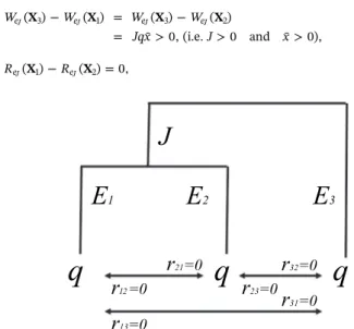
For the sake of clarity and tractability, we consider in the following the simplest ecosystem that allows us to compare the two biodiversity indices, that is a system composed of three species, N = 3, as depicted inFig. 1:

We assume that each species has Ei> 0 specific attributes that are

not shared with the two other species. Two species (here species 1 and 2) possibly share J ≥ 0 common attributes. We deduce that the in-formation about species dissimilarities is contained in the vector

= E E E J

D ( ,1 2, 3, )which we use in the following in order to assess our two criteria and discuss the impact of dissimilarity. This vector contains 1) information on the species attributes that are shared between any two or more species and 2) information on species attributes that are not shared.10_{We define d}

ij, the distance between species i and j, as the

number of attributes that are not shared by the two species, with

dij=dji. By assumption, species 3 has no common attributes with species

1 and 2. We have therefore d31= d13= E3+ E1+ J and

d32= d23= E3+ E2+ J. But we allow for the possibility that species 1

and 2 may have J ≥ 0 common attributes. So, d12= d21= E1+ E2.

2.3. Definitions of in situ Criteria for Conservation Priorities

The indices used in this paper are built on the ecological space presented so far. We denote Ω as the space of those parameters, and

=

e (Q, R D, ) (4)

as a particular element of this parameter space. This means in particular that the mapping that transforms efforts into probabilities is configured by parts of the information included in the vector e. In what follows, we emphasize this dependence using the subscript e whenever relevant, as in the notation P Xe( ).

2.3.1. Weitzman's Criterion for in situ Protection

Let Ve(S) be the diversity function of the (sub)set S of species given

by the length of the (sub)tree of species in S, i.e. the number of distinct attributes contained in S. It is important to note that this function is impacted by species dissimilarity but is not itself a measure of dissim-ilarity per se. Considering the three-species ecosystem presented above:

•

= + = + =

Ve({1}) E1 J, Ve({2}) E2 J, Ve({3}) E3, (5) that is, the total number of attributes (which are necessarily dis-tinctive) that characterize the species.

•

9_{Note that each element ofP( )X can be explicitly computed (seeAppendix A} for the three species case). To compute these elements, one must ensure that the result is between 0 and 1. Two possible strategies can satisfy this requirement: 1) assuming that estimates of the model parameters in real-world scenarios naturally guarantee this condition, 2) identifying an upper bound for con-servation efforts that guarantees this property. An algorithm exists for this purpose and is available from the authors on request.

10_{Dissimilarity information is conveyed in this vector and it applies to any} species collection set.

interrelationships on survival. While the ultimate causes of increased extinction in an interval of time may be abiotic, and might affect only some species directly, the intricate patterns of relationships among species in a community distribute the effects of changes in one species to others in its community. In order to take into account the impact of biotic interactions and conservation efforts s o a s t o g enerate

inter-dependent survival probabilities, we assume, along the lines of Courtois et al. (2014, 2018), a functional form to assess this probability. We denote , the interdependent survival prob-ability of species i and approximate this probprob-ability as a linear function of the protection effort xi measured in terms of probability variation,

and of rij ≡ ∂Pi/∂Pj, representing the marginal ecological impact of

species j on the survival probability of species i, with . We have then:

= + + = + + = + + V E E J V E J E V E J E ({1, 2}) , ({1, 3}) , ({2, 3}) , e 1 2 e 1 3 e 2 3 (6)

that is, the total number of distinctive attributes that characterizes the two species.

•

= + + +

Ve({1, 2, 3}) E1 E2 J E3, (7)

that is, the total number of distinctive attributes that characterizes the three species.

Weitzman's diversity index is the expected diversity function of the ecosystem, taking into account the extinction probability of each spe-cies. In a N-species ecosystem, this expected diversity index is:

=

We( )P _{S N} ( _{j S}Pj)( _{k N S}(1 Pk)) ( )V Se ₍₈₎

and it measures the expected length of the N-species evolutionary tree. When applied in our three-species ecosystem, the building blocks of the above expression are:

•

and the corresponding diversity is V ({1, 2, 3})e ,

•

P P P

(1 2)(1 3) 1, and the diversity is Ve({1}),

•

•

We deduce that Weitzman's expected diversity in the three species ecosystem reduces to:

= + + + +

We( )P P E1( 1 J) P E2( 2 J) P E3 3 P P J1 2 . (9) Since the goal is to rank conservation priorities while taking into account ecological interactions, the index must be modified in order to incorporate these interactions. We plug the relation between effort and probabilities, P X( ), into W(P). This yields Weitzman's in situ biodiversity

criterion, an expected diversity measure expressed as a function of

ef-fort: = + + + + W W P P E J P E J P E P P J X X X X X X X ( ) ( ( )), ( )( ) ( )( ) ( ) ( ) ( ) . e e e 1 1 2 2 3 3 1 2 (10)

2.3.2. Rao's Criterion for in situ Protection

Rao's index is the expected distance between any two species that are randomly drawn from a given set of species. In a N-species eco-system, this diversity index is:

= = = Re( )P P P d, i N j N i j ij 1 1 (11)

where dijis the distance between species i and j.Rao (1982)defines P as

a vector of probability distributions. For comparability of the two cri-teria and without loss of generality, we assume P is a vector of survival probabilities that is to be understood as the complement to a vector of extinction probabilities.11

In our three-species ecosystem, the index becomes:

= + + + + + + +

R( )P P P E1 2( 1 E2) P P E1 3( 1 E3 J) P P E2 3( 2 E3 J), (12) and the resulting relationship between diversity and effort is:

= + + + + + + + R P P E E P P E E J P P E E J X X X X X X X ( ) ( ) ( )( ) ( ) ( )( ) ( ) ( )( ). e 1 2 1 2 1 3 1 3 2 3 2 3 (13)

2.4. Simple in situ Protection Projects

Our objective is to compare three simple policies that concentrate efforts on either species 1, species 2 or species 3, referred to as

•

•

•

It follows that for a given vector of parameters e, project 1 is pre-ferred over project 2 and project 3, according to Weitzman's in situ criterion for protection iff:

We( )X1 max {We( ),X2 We( )}.X3 (14)

That is:

W xe( ¯, 0, 0) max We(0, ¯, 0),x We(0, 0, ¯).x (15)

Similarly, if Rao's criterion is used to rank priorities, then project 1 is favored iff:

Re( )X1 max { ( ),Re X2 Re( )},X3 (16)

or equivalently:

R xe(¯, 0, 0) max Re(0, ¯, 0),x Re(0, 0, ¯).x (17) Mutatis mutandis, the same kind of formal statements can indicate

the necessary and sufficient parameter conditions that lead to project 2 or 3 to be selected by each criterion. We are also in a position to study special cases in more detail, for their relevance to particular scenarios and/or because their simplicity is helpful in grasping the logic of the two in situ rankings.

The next section compares different optimization outcomes while keeping the analysis as simple as possible. It spares the reader the most technical details, which can be found inAppendices BandC. These appendices explicitly construct the Weitzman and Rao in situ indices in a three-species setting.

Fig. 1. Three species phylogenetic tree.

11_{It is interesting to note that in the ecology literature, this probability is} often assumed to be a frequency implying the additional constraint that

= P 1

i i . This leads to the assumption that relative abundance is per se a good

indicator of extinction risk, an assumption that is contradicted by several pa-pers, such asHarnik et al. (2012)orDulvy et al. (2005), as well as by most extinction risk assessment criteria that consider many other explanatory vari-ables.

3. Disentangling the Underlying Logic of in situ Priorities

If a species is selected for conservation efforts, it must be because it differs from the others in some way. For each criterion, this section ranks conservation policies under several parameter configurations e, chosen in order to isolate the role played by heterogeneity in particular factors. We show that the two criteria deliver opposite conservation recommendations when heterogeneity arises from autonomous survival probabilities Q, whereas they largely agree when heterogeneity arises from dissimilarities D, and ecological interactions R.

From a technical point of view, for a given vector of parameters e, the objective is essentially to compute:

W W R R X X X X ( ) ( ), ( ) ( ), e k e l e k e l

for k,l = 1,2, 3. All that remains is to analyze the signs of these dif-ferences. Though the calculations arrive at closed-form expressions and thus present no conceptual difficulties, the computational steps are nonetheless tedious. They were performed using a software designed for symbolic calculations (Xcas). Our Xcas spreadsheets are available upon request.

3.1. When the Criteria Diverge

3.1.1. The Influence of Autonomous Survival Probabilities(Q)

We start by analyzing cases in which autonomous survival prob-abilities are the unique source of heterogeneity among species, and examine the rankings generated by both criteria. We first consider a two-species ecosystem and subsequently extend the approach to a three-species ecosystem.

3.1.1.1. Two-species Ecosystem. Consider a class of conservation

problems summarized by the list of parameters eq, such that J ≥ 0, E1= E2= E, r12= r21= r, r13= r31= r23= r32= 0, and q1≠q2. The

phylogenetic tree associated with this ultrametric12 _{ecosystem is}

depicted inFig. 2:

Note that in this phylogenetic tree, we added additional information on autonomous survival probabilities qiat the end of each branch as

well as interaction parameters rij. Since we focus here on a two-species

ecosystem, vector Q and matrix R become:

q q r r Q R 0 , 0 0 00 0 0 0 e e 1 2 q q

and tedious computations produce:

= + W W Jx r q q X X ( ) ( ) ¯ (1 ) ( ), eq 1 eq 2 ₂ 1 2 ₍₁₈₎ = + R R Ex r q q X X ( ) ( ) 2 ¯ (1 ) ( ). eq 1 eq 2 ₂ 2 1 ₍₁₉₎

Expression (18) shows that Weitzman's ranking is sensitive to the dif-ference q1− q2only if J > 0, and becomes indifferent when J = 0. By

contrast, according to expression (19), the sensitivity of Rao's ranking to q2− q1does not depend on the value of J. Assuming J > 0, from Eqs.

(18) and (19), one can deduce the following proposition:

Proposition 1. Let the class of conservation problems be given by the list of

parameters eq. In this case, the two diversity criteria deliver opposite rankings:

•

•

How are these results explained? Ecological interactions are of little importance in this case, since both species serve identical ecological roles. These results are therefore consistent with the logic embodied in the indices alone. Weitzman's index seeks the longest expected tree. Recall that only one species is protected. If either species 1 or species 2 goes extinct, E attributes are lost but E + J attributes are saved. It is therefore sensible to allocate resources to protecting the species that is initially the most secure (i.e. the species whose autonomous survival probability is the highest), unless J = 0, in which case Weitzman's criterion would clearly be indifferent regarding which species should be allocated protection efforts. Regarding the Rao criterion, the question is: how can one choose the combination of probabilities that leads to the highest expected diversity? Put more precisely, in this two-species problem, Rao seeks the largest product P1(X)P2(X). This is best achieved

when a conservation policy helps the fragile species, i.e. the species most likely to become endangered. Protection efforts are optimally al-located where the marginal impact is highest, therefore to species i if Pi

≤ Pj, to species j if Pj≤ Pi.

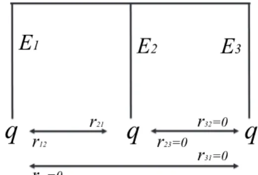
3.1.1.2. Three-species Ecosystem. These results are robust to the

introduction of a third species, provided that the only source of heterogeneity among species continues to be their autonomous survival probability. To avoid dissimilarities as a source of heterogeneity, we retain the same distances between species, and a good ecosystem candidate is the simple ultrametric case where J = 0,

E1= E2= E3= E, and where q3can take any arbitrary value. This leads

us to consider a slightly different list of parameterse_q. The phylogenetic tree and associated information that characterizes this ecosystem is depicted inFig. 3:

From Xcas computations, usingAppendices BandC, one finds:

= =

Weq( )X1 Weq( )X2 Weq( )X1 Weq( )X3 0. (20) In other words, Weitzman's criterion proves to be indifferent between the three conservation policies. The reason for this indifference is that in this peculiar ecosystem, species have no common attributes. This makes conservation effort toward one species versus the other perfectly substitutable. Considering G > 0, shared attributes between the three species would modify this result — making the criterion in favor of investing in the most robust species. As for Rao's criterion, one has:

= + R R Ex r q q X X ( ) ( ) 2 ¯ ( 1) ( ), eq 1 eq 2 ₂ 2 1 ₍₂₁₎

Fig. 2. Two-species ultrametric tree with J > 0.

= + R R Ex r q q X X ( ) ( ) 2 ¯ ( 1) ( ), eq 1 eq 3 ₂ 3 1 ₍₂₂₎ = + R R Ex r q q X X ( ) ( ) 2 ¯ ( 1) ( ), eq 2 eq 3 ₂ 3 2 ₍₂₃₎

from which one directly deduces that the most fragile species ranks highest, which again confirmsProposition 1. Next, we examine the role of dissimilarity, discarding any heterogeneity in terms of autonomous survival probabilities and species interactions.

3.2. When the Criteria Converge

3.2.1. The Influence of Attributes Dissimilarity

Attribute dissimilarities are embedded in the two indices in different ways. In order to analyze the role played by D, the simplest ecosystem to consider is a three-species ultrametric ecosystem in which species 1 and 2 share J common attributes and where E1= E2= E and

E3= E + J. Species 3 is more dissimilar than the two other species.

Consider further that q1= q2= q3= q > 0 and rij= 0. In the absence

of ecological interactions and in the ultrametric case where

E1= E2= E,E3= E + J, the matrices Q and R become:

q q q Q , R 0 0 00 0 0 0 0 0 , eJ eJ

and this ecosystem, denoted by parameter vector eJ, is depicted in Fig. 4:

Xcas computations deliver the following key pieces of information:

= WeJ( )X1 WeJ( )X2 0, = = > > > W W W W Jqx J x X X X X ( ) ( ) ( ) ( ) ¯ 0, (i.e. 0 and ¯ 0), eJ 3 eJ 1 eJ 3 eJ 2 = ReJ( )X1 ReJ( )X2 0, = = > R R R R Jqx X X X X ( ) ( ) ( ) ( ) 2 ¯ 0. eJ 3 eJ 1 eJ 3 eJ 2

A conclusion immediately emerges:

Proposition 2. Let the class of conservation problems be given by the list of

parameters eJ. In this three-species ecosystem where dissimilarities are the only source of heterogeneity among species, the two diversity criteria deliver the same rankings:

•

•

This result seems intuitive. If only species 1 (or 2) disappears, there remains 2(E + J) attributes. But if only species 3 disappears, the number of remaining attributes decreases to a lower 2E + J. In Appendix D.1, however, we show that the property emphasized in

Proposition 2is fragile. More precisely, it holds only when ecological interactions are not too strong (even if ecological interactions are not a source of heterogeneity).

3.2.2. The Influence of Ecological Interactions

Incorporating this dimension in the model is an attempt to account for the complexities of the web of life. For instance, the interactions between two species can be considered unilateral, e.g. species 1 impacts species 2 but not vice versa, or bilateral, e.g. species 1 impacts species 2 and species 2 impacts species 1. In a two-species system, there are 22_{= 4 interaction possibilities to consider. As soon as one contemplates}

a three-species ecosystem, however, there are 33_{= 27 potential}

pair-wise interactions between species (not even taking into account the added complexity that could be introduced by varying the intensity of each of these ecological interactions). It is evident that the number of interaction possibilities quickly explodes with the number of species in the system. In the face of this complexity, our strategy will be to focus on two illustrative cases of particular interest. To simplify matters, we assume that dissimilarities play no role and consider the simplest pos-sible ecosystem.

3.2.2.1. Two-species Ecosystem. Consider first a situation with two

interacting species, 1 and 2. The third species does not interact with species 1 or with species 2 and is considered extinct. We assume the two species share no common attributes, but possess a similar number of specific attributes, i.e. E1= E2= E and J = 0. The phylogenetic tree

associated to this ecosystem is depicted inFig. 5:

Consider a parameter vector eR2where r12≠r21, all other rijbeing

equal to zero, and q1= q2= q,q3= 0. The matrices Q and R become:

q q r r Q R 0 , 0 0 0 0 0 0 0 . e e 12 21 R2 R2

Computing the biodiversity criteria reveals:

Fig. 3. Three-species ultrametric case with J = 0.

= W W Ex r r r r X X ( ) ( ) ¯ 1 ( ), e 1 e 2 12 21 21 12 R2 R2 ₍₂₄₎ = + R R Ex q x r r r r X X ( ) ( ) 2 ¯ (2 ¯) (1 ) ( ). e 1 e 2 12 21 2 21 12 R2 R2 ₍₂₅₎

From these expressions, we establish the following proposition:

Proposition 3. Let the class of conservation problems be given by the list of

parameters eR2. The two criteria deliver the same ranking of policies X1and

X2. They recommend preserving the species that has the largest marginal impact on the survival of the other species:

W W r r R R r r X X X X ( ) ( ) , ( ) ( ) . e e e e 1 2 21 12 1 2 21 12 R R R R 2 2 2 2

In this case, the two criteria recommend preserving the species that has the largest marginal effect on the survival probability of the other species, a result that confirms a previous finding from Baumgärtner (2004a). Each criterion aims to maximize the survival probability of the ecosystem as a whole. This result can be illustrated using the principal categories of interactions between our two species.

i) Predation: species 2, a predator, feeds on species 1, its prey.

By definition, we have r21> 0 and r12< 0. Both criteria

re-commend preserving the prey – here species 1 – since its interaction coefficient is larger (r12< 0 < r21).

ii) Mutualism: species 1 and 2 have a positive impact on each

other. By definition, we have r12> 0 and r21> 0. Both

cri-teria recommend preserving the species with the largest marginal benefit on the survival probability of the other species.

iii) Competition: species 1 and 2 rely on a common resource in the

same territory that cannot fully support both populations. By definition, we have r12< 0 and r21< 0. Both criteria

re-commend preserving the species with the lowest negative impact on the other species.

3.2.2.2. Three-species Ecosystem. When a third species is introduced,

the impact of species interactions on the criteria recommendations is more difficult to study, as there is now an interplay of effects due to more complex interactions in the system. In order to illustrate this complexity, we consider a simple ecosystem of three interacting species characterized by unilateral interactions. We assume a single species, say species 1, impacts the two other species, but these two species impact neither each other nor species 1. For example, species 1 is a predator that negatively impacts two preys, species 2 and 3, but does not rely on them to survive due to the availability of other food sources, i.e. ri1< 0, ri2= ri3= 0. Species 1 could also be the prey of the two other species

without being negatively impacted by them, i.e. ri1≥ 0, ri2= ri3= 0.

Define a vector eR3 such that E1= E2= E3= E, J = 0,

q1= q2= q3= q and all interaction coefficients beside r21and r31are

null. The phylogenetic tree associated with this three-species ultra-metric ecosystem is depicted inFig. 6:

Here, the only distinction between the three species is how they interact. Matrices Q and R become:

q q q rr Q , R 0 0 0 0 0 0 0 . e e 21 31 R3 R3

The relative performance of alternative projects is measured by:

= + WeR3( )X1 WeR3( )X2 Ex r¯ (21 r31), (26) = + WeR3( )X1 WeR3( )X3 Ex r¯ (21 r31), (27) = WeR3( )X2 WeR3( )X3 0, (28) = + + + + + R R Ex r r q x r q x r q x X X ( ) ( ) 2 ¯ (2 ¯) (3 ¯) (2 ¯) , e 1 e 2 21 31 21 31 R3 R3 (29) = + + + + + R R Ex r r q x r q x r q x X X ( ) ( ) 2 ¯ (2 ¯) (2 ¯) (3 ¯) , e 1 e 3 21 31 21 31 R3 R3 (30) = ReR3( )X2 ReR3( )X3 2 ¯ (Exq r31 r21). (31) Weitzman's criterion recommends preserving species 1 rather than species 2 or 3 iff:

>

WeR3( )X1 max (WeR3( ), W ( )).X2 eR3X3

The above expressions (26) and (27) show that this is true iff

r21+ r31> 0, that is, if the cumulative impact of species 1 on the

survival probability of the two other species is larger than the cumu-lative impact of these species on all other species (which is null here as we assume r12= r13= r23= r32= 0). This result confirms

Proposition 3, as it recommends allocating conservation efforts to the species that is the most beneficial (or the least detrimental) to the survival of all of the other species in the ecosystem.

Similarly, Rao's criterion recommends preserving species 1 rather than species 2 and 3 when:

>

ReR3( )X1 max (ReR3( ),X2 ReR3( )).X3

From expressions (29) and (30), this is true iff

+ + + + + >

r r21 31(2q x¯) r31(2q x¯) r21(3q x¯) 0 and r r21 31(2q+x¯)+ + + + >

r21(2q x¯) r31(3q x¯) 0. In the case in which species 1 has a po-sitive impact on species 2 and 3, preservation effort is allocated to species 1. When either of the above inequalities do not hold, inter-preting the criterion becomes more difficult. In this case, effort is then allocated to the species that is (negatively) impacted to a greater degree by species 1. Again, we find a confirmation of the result presented in

Proposition 3. However, the decision rule depicted here is no longer a simple additive formula, but a combination of additive and multi-plicative components (r21r31), making interpretation difficult. Adding

interrelations or additional species in the analysis greatly increases complexity through multiplicative effects (i.e. complementarities).

4. Interactions Between Effects

When heterogeneity arises from several dimensions at once, all of the previous criteria logics are mingled and interpreting the results becomes very challenging indeed. A fairly detailed analysis for the in-terested reader is given inAppendix D. Here, we briefly discuss a case in point. We let species differ in both autonomous survival probabilities (the qi’s) and ecological interactions (the rij’s). Recall that, all else being

equal, the Weitzman criterion tends to generate recommendations that protect robust species that are a priori the least concerned by extinction (with the largest qi), whereas the Rao criterion generally favors fragile

species likely to be the most threatened species. On the other hand, on the basis of ecological interactions only, both criteria recommend that conservation efforts be allocated to the species with the largest positive impact on the ecosystem. Thus, an initial dissonance in rankings due to the qi’s can vanish if this ecological interactions effect prevails. This is

indeed the case and can be explored formally. See Appendix D.3.

5. Summary and Illustration

Considering a binary choice between investing in the conservation of one of two species (in an ecosystem that may contain more than two or three species) and denoting these two species A and B, the main results we obtain in the paper are summarized inTable 1:

Abusing notations, we write A > B when species A has a greater survival probability (respectively attribute dissimilarity or overall net positive impact on the ecosystem through species interactions) than species B, and we write A ≻ B when the criterion favors the protection of species A. Rankings are generated under the assumption that ev-erything else is equal, meaning that, in line 1 for example, we assume that species A has a greater survival probability than species B, but that the two species are symmetric in all other aspects.

We observe that the two criteria converge regarding attribute dis-similarity (D) and species interactions (R). Both favor species that contribute more to the diversity of the attributes contained in the ecosystem, as well as species that impart the greatest benefits, or least harm, to the ecosystem. Conversely, the criteria diverge regarding au-tonomous survival probability (Q) and therefore regarding how they value the relative robustness of species. While the Weitzman criterion recommends protecting the species that is a priori the least prone to extinction, the Rao criterion finds the opposite, recommending that conservation efforts should focus on the species that is more likely to become endangered. With respect to conservation policy, it therefore turns out that the Weitzman criterion can be considered a triage deci-sion concept that seems particularly appropriate for situations invol-ving massive extinction potential and a limited conservation budget. Conversely, the conservation philosophy underlying Rao's is to allocate funds toward the most threatened species, disregarding the chances of successfully preventing extinction. It is therefore particularly appro-priate in the context of large budgets or low extinction.

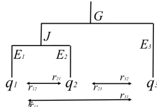
We conclude the paper with an illustration of our results based on a simple simulation. Again, we consider an ecosystem that is composed of three species, as described inFig. 7:

We assume that species 3 is more distinctive than the two others and we arbitrarily set G = 50, J = 90, E3= 100 and E1= E2 = 10.

In what follows, we examine the binary choice of preserving one of two species contained in this ecosystem by gradually adding complexity to the parameter space considering first heterogeneity in autonomous survival probabilities (Q) and second in species interactions (R). We assume for the moment that rij= 0, ∀i,j, meaning that there is no

in-teraction between species. We set q3= 0.4 meaning that species 3 is

vulnerable13_{, and we assume that the autonomous survival probability}

of species 1 and 2 may oscillate between 0 and 1, i.e. between critically

endangered and most robust (IUCN species status is provided in

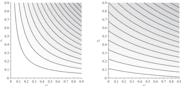
Appendix E). We focus on the choice of investing either in species 1 or 2, that is in the two less distinctive species composing this ecosystem. Isoquant curves are useful to illustrate how the two criteria value re-lative autonomous survival probabilities between the two species. An isoquant here is a contour line drawn through the set of points at which the same value of the criterion is obtained while changing the auton-omous survival probabilities of the two species. Each isoquant depicts then the set of couples q1,q2that forward the same criterion value.

Darker grey zones depict higher criteria levels, meaning that the higher the isoquant, the higher the criterion value. We observe that the Weitzman's criterion isoquants are concave with a slope greater than − 1 above the bisectrix. The Rao's criterion isoquants are convex with a slope less than − 1 above the bisectrix. It follows that in order to reach a superior isoquant and therefore a higher diversity, if q2> q1 (i.e.

above the bisectrix line), Weitzman criterion recommends investing in the protection of species 2 (AB < AC), while Rao's criterion re-commends investing in the protection of species 1 (AC < AB). Conversely, below the bisectrix, Weitzman's criterion recommends in-vesting in q1, while Rao's criterion recommends investing in q2. We

confirm the result that, all else equal, Weitzman's criterion favors robust species, while Rao's criterion favors fragile ones.

Let us now increase the complexity of the problem to illustrate how the two criteria value distinctiveness (D). As species 3 is assumed to be more distinctive than the other two that share J common attributes, we now focus on the binary choice of either protecting species 1 or pro-tecting 3. Again, we assume that no interactions exist between species,

rij= 0∀i,j, but we now let q1and q3vary between 0 and 1. We assume

that q2is equal to either 0.01 or 0.99, i.e. the canonical cases where

species 2 is either critically endangered or extremely robust. In the first case, as species 2 is almost extinct, species 1 is almost as distinctive as species 3. In the second case, species 3 is more distinctive than species 1 as the J attributes are always secured by species 2. Isoquants for the two cases and the two criteria are depicted inFigs. 9and10.

We observe that when species 2 is least concerned by extinction (right-hand graphs), the slopes of the isoquants flatten, indicating that both criteria favor the protection of species 3. Notice that here, the impact of dissimilarity on criteria rankings outweighs the impact of autonomous survival probability. Even if species 1 is fragile, the two criteria recommend preserving species 3, as the J attributes of species 1 will continue to exist in the ecosystem via species 2. Interestingly, we observe that if species 2 is almost extinct, we confirm previous insights regarding autonomous survival probability.14

To conclude, we illustrate the impact of species interactions on the recommendations made by the two criteria. Considering again the binary choice between preserving species 1 or 2 and assuming q3= 0.4,

i.e. the parameter considered in the case depicted inFig. 8, we compare Weitzman criterion Rao criterion

Survival probability (Q) If A > B, then A ≻ B B ≻ A Attribute dissimilarity (D) If A > B, then A ≻ B A ≻ B Species interaction (R) If A > B, then A ≻ B A ≻ B

J

G

E

E

E

q

1

_r

q

2

_r

r

q

3

rr

r

r

Fig. 7. Three-species ultrametric case with J > 0 and G > 0.

13_{Note that we could assume q3to be any value between 0 and 1.}

14_{The Weitzman criterion is almost indifferent between preserving the two} species since G is small, making efforts to protect each species almost perfectly substitutable.

Table 1

Fig. 8. Isoquants: Weitzman (left), Rao (right).

Fig. 9. Weitzman's criterion isoquants: q2= 0.01 (left), q2= 0.99 (right).

the no interaction case (rij= 0∀i,j) and the predator-prey case where

species 2 is the predator of species 1 (r12= −0.5 and r21= 0.3, and all

remaining rij= 0). Isoquants for the two cases and the two criteria are

depicted inFigs. 11and12.

Notice that when introducing species interactions, here a predator-prey relationship between species 2 and 1, both criterion's isoquants become steeper, meaning that the preservation of species 1 becomes more likely. This illustratesProposition 3, according to which the cri-teria tend to allocate conservation efforts to the species that imparts the most benefits to the ecosystem. Here, species 1 is the prey and its presence positively impacts the survival probability of species 2.

6. Conclusion

This paper modifies Weitzman's and Rao's biodiversity indices, in-corporating information about ecological interactions in order to render the models more appropriate for in situ protection plans. Using the re-sulting Weitzman's and Rao's in situ criteria, a simple framework allows us to analyze and compare the recommended conservation plans. For each in situ criterion, we are able to disentangle the role played by three factors: i) autonomous survival probabilities Q, ii) ecological interac-tion R and, iii) dissimilarity D. We consider these factors both in strict isolation and in combination.

The analysis generates three important outcomes:

1. The two criteria, originating from different academic fields, com-bine information on Q, R and D in different ways in order to mea-sure biodiversity. As a consequence, they do not systematically de-liver the same conservation recommendations. They diverge when differences between species arises from autonomous survival prob-abilities, whereas they largely agree when species heterogeneity arises from dissimilarities and/or ecological interactions.

2. When ecological interactions matter for the ranking, the favored species is the one that imparts the most benefits, or least harm, to the ecosystem. In general, the introduction of ecological interactions among more than two species can lead to complex conclusions. 3. When the three elements are combined, the policy recommended by

each criterion reveals a specific trade-off between Q, R and D. From a practical point of view, an interesting follow-up to this re-search would be to consider any number of species, among which only a subset can feasibly receive protection. The analytical interpretation of the rankings in this case would probably be lost, but such an analysis does not seem to pose any computational problems.

At a more fundamental level, further consideration should be given to the objectives of conservation policies. Each biodiversity index is, by construction, a measure of a certain vision of biodiversity and therefore of conservation. It is interesting to learn that, all else being equal, there is a tendency for Weitzman's criterion to favor robust species, and for

Fig. 11. Weitzman's criterion isoquants: no interaction case (left), predator-prey case (right).

Acknowledgments

The article greatly benefited from helpful and detailed comments by three anonymous referees and the Editor in charge, Patricia Perkins. We also thank Jean Marc Bourgeon, Luc Doyen, Kate Farrow, Guy Meunier, Raphael Soubeyran, Tim Swanson, Alban Thomas, and the seminar/ conference participants of CEE-M (Montpellier), Crest (Paris), Gael (Grenoble), BIOECON 2018 (Cambridge), WCNRM 2017 (Barcelona), Journes INRA-IRSTEA 2018 (Montpellier). Financial support from INRA-AFB Convention 2016–2018 and ANR Green-Econ (ANR-16-CE03-0005) is acknowledged.

Solving the system Eq. (2) of ecological interactions for P1,P2and P3as functions of = x x xX ( , ,1 2 3)Tgives:

= + + + + + + + P q x r r q x r r r q x r r r r r r r r r r r r r r r X ( ) ( )(1 ) ( )( ) ( )( ) 1 1 1 1 23 32 2 2 12 13 32 3 3 12 23 13 23 32 12 21 13 31 12 31 23 21 13 32 (32) = + + + + + + + P q x r r q x r r r q x r r r r r r r r r r r r r r r X ( ) ( )(1 ) ( )( ) ( )( ) 1 2 2 2 13 31 1 1 21 31 23 3 3 21 13 23 23 32 12 21 13 31 12 31 23 21 13 32 (33) = + + + + + + + P q x r r r q x r r r q x r r r r r r r r r r r r r r X ( ) ( )( ) ( )( ) ( )(1 ) 1 . 3 1 1 31 32 21 2 2 12 31 32 3 3 12 21 23 32 12 21 13 31 12 31 23 21 13 32 (34)

The probability of species 1 can be described as a combination of each species' intrinsic survival probability augmented by protection effort, as articulated through direct and indirect interactions among species.

In vector notations, probabilities as functions of efforts are:

= + P P P P X X X X Q X ( ) ( ) ( ) ( ) *( ). 1 2 3 with = I R[ ]1_.

Appendix B. Three-species Weitzman's Criterion for in situ Protection When Distances are Ultrametric

In a three-species model, considering parameter vector =e (Q, R D, ) , Weitzman's expected diversity as a function of efforts is:

= + + + + W W P P E J P E J P E P P J X X X X X X X ( ) ( ( )), ( )( ) ( )( ) ( ) ( ) ( ) . e 1 1 2 2 3 3 1 2

Assuming distances are ultrametric, E1= E2= E and E3= E + J, with E > 0 and J ≥ 0, we have:

= + + +

We( )X [ ( )P1 X P2( )X P3( )](X E J) P1( ) ( ) .X P2 XJ

Using Eqs. (32), (33)and (34), we obtain the following value for a vector of effort X:

= + + + + + + + + + + + + + + + + + + + + + + + + + + + + + + W E J q x r r r r r r r r q x r r r r r r r r q x r r r r r r r r J q x r r q x r r r q x r r r q x r r q x r r r q x r r r X ( ) 1 ( ) ( )( ) ( )( ) ( )( ) ( )(1 ) ( )( ) ( )( ) ( )(1 ) ( )( ) ( )( ) e 1 1 21 31 32 21 31 23 23 32 2 2 12 32 13 32 12 31 13 31 3 3 13 23 12 23 21 13 12 21 1 1 23 32 2 2 12 13 32 3 3 12 23 13 2 2 13 31 1 1 21 31 23 3 3 21 13 23 with =(1 r r23 32 r r12 21 r r13 31 r r r12 31 23 r r r21 13 32)2.

Appendix C. Three-species Rao's Criterion for in situ Protection When Distances are Ultrametric

For parameter vector =e (Q, R, D) , and givenP( )X * Q( +X), Rao's index for in situ protection is:

= + + + + + + + = + + + + R P P E E P P E E J P P E E J P P P P P P E P P P J X X X X X X X X X X X X X X X X ( ) ( ) ( )( ) ( ) ( )( ) ( ) ( )( ) 2[( ( ) ( ) ( ) ( ) ( ) ( )) ( ( ) ( )) ( ) ] e 1 2 1 2 1 3 1 3 2 3 2 3 1 2 1 3 2 3 1 2 3

and considering ultrametric distances such that E1= E2= E and E3= E + J, with J ≥ 0 and E > 0, we obtain:

= + + + +

Re( )X 2[( ( ) ( )P1 X P2 X P1( ) ( )XP3 X P2( ) ( ))X P3 X E ( ( )P1X P2( )) ( ) ].X P3 X J

Using system Eqs. (32), (33), and (34), the value of the criterion for a vector of effort X is: Rao's criterion to favor fragile ones. The choice of one criterion over the

other therefore depends on the policy perspective adopted. If the available conservation budget is large and the opportunity exists to save a great many species, then Rao's criterion is the most appropriate choice. If the conservation budget is limited and the potential for spe-cies extinction is as drastic as that of the narrative of Noah's Ark, Weitzman's criterion should be seriously considered. In order to arrive at a unique policy solution, it will therefore be necessary to develop a criterion for selecting from among biodiversity indices themselves. The present paper demonstrates that such a meta-criterion would essentially determine the trade-off t hat i s u ltimately m ade b etween r obust and fragile species in conservation management.

= + + + + + + + + + + + + + + + + + + + + + + + + + + + + + + + + + + + + + + + + + + + + + + + + + + + + + + + + + + + + R E q x r r q x r r r q x r r r q x r r r r r r q x r r r r r q x r r r r r E q x r r r q x r r q x r r r q x r r r r r q x r r r r r r q x r r r r r E J q x r r r q x r r r q x r r q x r r r r r q x r r r r r q x r r r r r r X ( ) 1 ( )(1 ) ( )( ) ( )( ) ( )( ) ( )(1 ) ( )( 1 ) ( )( ) ( )(1 ) ( )( ) ( )(1 ) ( )( ) ( )( 1 ) ( ) ( )( ) ( )( ) ( )(1 ) ( )(1 ) ( )( 1 ) ( )( ) e 1 1 23 32 2 2 12 13 32 3 3 12 23 13 1 1 21 31 23 31 21 32 2 2 13 31 32 31 12 3 3 23 21 13 21 12 1 1 21 31 23 2 2 13 31 3 3 23 21 13 1 1 23 32 31 21 32 2 2 12 13 32 32 31 12 3 3 12 23 13 21 12 1 1 31 21 32 2 2 32 31 12 3 3 21 12 1 1 23 32 21 31 23 2 2 12 13 32 13 31 3 3 12 23 13 23 21 13 with =(1 r r23 32 r r12 21 r r13 31 r r r12 31 23 r r r21 13 32)2.

Appendix D. Interactions Between Effects

D.1. Autonomous Survival Probabilities and Dissimilarities

Let us examine the combination of autonomous survival probabilities and dissimilarity. Consider a slight departure from the parameter con-figuration eqinSection 3.1.1. In the new list of parameters eqJ, the unique difference arises from parameter J, which is no longer null, J > 0, and rij= r, when i≠j. The vector Q and the matrix R are:

q q q r r r r r r Q , R 0 0 0 . e e 1 2 3 qJ qJ

The relative performance of policies can be deduced from:

= + W W Jx r q q X X ( ) ( ) ¯ (1 ) ( ), eqJ 1 eqJ 2 ₂ 1 2 ₍₃₅₎ = + + + + W W Jx r q q x q r r r X X ( ) ( ) ¯ [ ( ) (1 )] (1 ) (2 1) , eqJ 1 eqJ 3 1 3 ₂ 2 ₍₃₆₎ = + + + + W W Jx r q q x q r r r X X ( ) ( ) ¯ [ ( ) (1 )] (1 ) (2 1) , eqJ 2 eqJ 3 2 3 ₂ 1 ₍₃₇₎ = + R R Ex r q q X X ( ) ( ) 2 ¯ (1 ) ( ), eqJ 1 eqJ 2 ₂ 2 1 ₍₃₈₎ = + + + + R R Jx r q q q rx q q q r r Ex r q q X X ( ) ( ) 2 ¯ [ (3 ) ¯ ( )] (1 ) (2 1) 2 ¯ (1 ) ( ), e 1 e 3 3 1 2 ₂ 3 1 2 2 3 1 qJ qJ (39) = + + + + R R Jx r q q q rx q q q r r Ex r q q X X ( ) ( ) 2 ¯ [ (3 ) ¯ ( )] ( 1) (2 1) 2 ¯ (1 ) ( ). e 2 e 3 3 1 2 ₂ 3 1 2 2 3 2 qJ qJ (40) When the choice to be made involves species 1 and 2, we again find that Weitzman's logic favors robust species, whereas Rao's index favors weak species.

The conclusions are more nuanced when a third species is introduced, and they depend on the importance of ecological interactions: Weitzman's index favors species 3 only if r < 1/215_{. In other words, dissimilarity prevails when ecological interactions are not too strong. The conclusion is even}

more complex when it comes to Rao's index. Whatever the recommendation, it is reversed when r crosses the value 1 /2. As a particular case, now let the autonomous probabilities of survival be identical. The relative policy performances (Eqs. (35) to (40)) simplify to:

= WeqJ( )X1 WeqJ( )X2 0, (41) = + + + W W Jx r q x q r r X X ( ) ( ) ¯ [ ( ¯) ] (1 ) (2 1), eqJ 1 eqJ 3 _{2 (42)} = + + + W W Jx r q x q r r X X ( ) ( ) ¯ [ ( ¯) ] (1 ) (2 1), eqJ 2 eqJ 3 _{2 (43)} = ReqJ( )X1 ReqJ( )X2 0, (44)