HAL Id: lirmm-01541930
https://hal-lirmm.ccsd.cnrs.fr/lirmm-01541930
Submitted on 19 Jun 2017
HAL is a multi-disciplinary open access
archive for the deposit and dissemination of sci-entific research documents, whether they are pub-lished or not. The documents may come from teaching and research institutions in France or
L’archive ouverte pluridisciplinaire HAL, est destinée au dépôt et à la diffusion de documents scientifiques de niveau recherche, publiés ou non, émanant des établissements d’enseignement et de recherche français ou étrangers, des laboratoires
A graph-based approach to detect spatiotemporal
dynamics in satellite image time series
Fabio Güttler, Dino Ienco, Jordi Nin, Maguelonne Teisseire, Pascal Poncelet
To cite this version:
Fabio Güttler, Dino Ienco, Jordi Nin, Maguelonne Teisseire, Pascal Poncelet. A graph-based approach to detect spatiotemporal dynamics in satellite image time series. ISPRS Journal of Photogramme-try and Remote Sensing, Elsevier, 2017, 130, pp.92-107. �10.1016/j.isprsjprs.2017.05.013�. �lirmm-01541930�
A graph-based approach to detect spatiotemporal dynamics in
1
satellite image time series
2
Fabio Guttlera,b,∗, Dino Iencoa, Jordi Ninc, Maguelonne Teisseirea, Pascal Ponceletd
3
aUMR TETIS, Irstea, 500 rue Jean-Franois Breton F-34093, Montpellier, France 4
bDYNAFOR, INP-EI PURPAN, INP-ENSAT, INRA, University of Toulouse, 75 voie du TOEC, 31076 5
Toulouse, France 6
cUniversitat Politcnica de Catalunya (BarcelonaTech), Barcelona, Spain 7
dUniversity of Montpellier and LIRMM Laboratory - 860 rue de Saint Priest F-34095 Montpellier, France 8
Abstract 9
Enhancing the frequency of satellite acquisitions represents a key issue for Earth Obser-vation community nowadays. Repeated obserObser-vations are crucial for monitoring purposes, particularly when intra-annual process should be taken into account. Time series of images constitute a valuable source of information in these cases. The goal of this paper is to pro-pose a new methodological framework to automatically detect and extract spatiotemporal information from satellite image time series (SITS).Existing methods dealing with such kind of data are usually classification-oriented and cannot provide information about evolutions and temporal behaviors. In this paper we propose a graph-based strategy that combines object-based image analysis (OBIA) with data mining techniques. Image objects computed at each individual timestamp are connected across the time series and generates a set of evolution graphs. Each evolution graph is associated to a particular area within the study site and stores information about its temporal evolution. Such information can be deeply explored at the evolution graph scale or used to compare the graphs and supply a general picture at the study site scale. We validated our framework on two study sites located in the South of France and involving different types of natural, semi-natural and agricultural areas. The results obtained from a Landsat SITS support the quality of the methodological approach and illustrate how the framework can be employed to extract and characterize spatiotemporal dynamics.
Keywords: Satellite Image Time Series, Monitoring, OBIA, Data Mining, Graph-based
10
techniques, Land-cover. 11
∗corresponding author
Email addresses: [email protected] (Fabio Guttler ), [email protected] (Dino Ienco), [email protected] (Jordi Nin), [email protected] (Maguelonne Teisseire), [email protected] (Pascal Poncelet)
1. Introduction 12
Nowadays, satellite image time series (SITS) is a powerful source of information for 13
monitoring purposes. Repeated satellite observations allow to follow the evolution (e.g. 14
growing season, land-cover modifications) of a given area over the time in a systematic way. 15
When repeatability and homogeneity of satellite observations are guaranteed it becomes 16
possible to detect spatiotemporal evolutions and deduce their related dynamics (Bonn, 1996). 17
However, the interpretation and the cross-comparison of several satellite images quickly 18
become challenging. 19
Advanced methods used to process multitemporal optical imagery are related to tra-20
jectory analysis. In this context, high-temporal frequency SITS from coarse to moderate 21
sensors, such as MODIS, are used to model temporal signatures and detect anomalies or 22
trends (Lunetta et al., 2006; Verbesselt et al., 2010; Cai and Liu, 2015). Although powerful, 23
these methods are hardly adaptable in finer spatial scales applications where the number 24
of images available is lower and the temporal sampling is irregular. However, several local 25
scale applications need high frequency of observations at intra-annual basis. Mapping and 26
monitoring natural and agricultural areas with an enhanced revisit capacity allows monitor-27
ing phenology states, agricultural practices and seasonal processes. Recent reviews about 28
conservation monitoring (Nagendra et al., 2013) and Natura 2000 habitat monitoring (Van-29
den Borre et al., 2011) pointed out remote sensing as a strong, but still underexploited, 30
tool. 31
In the literature, methods used to process multitemporal optical imagery are commonly 32
grouped under the change detection label. In a pioneer review article, Singh (1989) defined 33
change detection as the process of identifying differences in the state of an object or phe-34
nomenon by observing it at different times. The author also categorised the main change 35
detection techniques in ten different groups. A critical review about change detection meth-36
ods in ecosystem monitoring was provided by Coppin et al. (2004). More recently, Hussain 37
et al. (2013) expanded the change detection categories previously proposed by Singh (1989), 38
including object-based change detection (OBCD) techniques. Regarding this last point, the 39
works of Chen et al. (2012) and Blaschke (2005) provided a deep overview of the available 40
OBCD methods. 41
Considering SITS of optical imagery, we can highlight twomain limitations in the current 42
literature. Firstly, most of the existing methods focus their efforts on bi-temporal change 43
detection situations, i.e. the study of temporal evolutions taking place between two dates. 44
Usually, these methods include post-classification comparison (Yuan et al., 2005), image dif-45
ferencing (Lu et al., 2005), composite analysis (B. Descle, 2006), linear transformation (Qin 46
et al., 2013) and change vector analysis (Malila, 1980). Secondly, the majority of works 47
explored mainly pixel-based strategies (Petitjean et al., 2012; Inglada et al., 2015) whereas 48
object-based image analysis (OBIA) are still among open challenges in remote sensing anal-49
ysis (Blaschke et al., 2014; Chen et al., 2012). 50
Petitjean et al. (2012) constructed vector images from SITS and used classical unsuper-51
vised classification (k-means) at pixel level. The originality of the approach consisted in 52
the integration of spatial relationships between pixels. Each pixel was enriched by some 53
contextual attributes coming from individual image segmentations performed at each times-54
tamp. In this case, the temporal behavior (based on 15 FORMOSAT-2 images acquired in 55
the same year) was used to assign a unique land cover label (mainly crops) to each pixel. 56
These labels, derived from ground reference data, are static (e.g. corn) and do not describe 57
dynamics (e.g. bare soil -> growth of corn -> harvest); therefore it is not possible to per-58
form further analysis, or monitoring, related to the intra-annual evolutions. Inglada et al. 59
(2015) evaluated the performance of state-of-the-art supervised classification methods for 60
generating accurate crop type maps on 12 sites spread all over the world. The classification 61
strategy giving the best results combined pixel-based temporal linear interpolation and fea-62
ture extraction (radiometry derived features only). In this case, SITS were composed of a 63
variable number of SPOT-4 and Landsat-8 images (from 9 to 41 images depending on the 64
site) acquired in the same year. In general, important amounts of ground reference data 65
(from several dozens to a few thousands of hectares) were necessary for training the classifier 66
and achieving accurate results. Also here, the process chain generates a single outcome (i.e. 67
a map) representing static land cover classes. This flat representation, alone, is not able to 68
describe the evolutions and the temporal behaviors behind each class label. 69
Differently from previous approaches that mainly focus on the classification and/or de-70
tection of abrupt changes between consecutive images, this paper aims to describe a new 71
methodology to explore SITS data detecting and describing spatiotemporal entities/phenomena 72
existing in the study area. More in detail, given a time series of remote sensing images and 73
an associated segmentation, our objectives are to: (i) detect the set of spatiotemporal enti-74
ties/phenomena existing in the study area and (ii) supply a spatiotemporal description for 75
each of them. To this end, we propose an hybrid methodology combining OBIA and data 76
mining techniques. Our proposal firstly identifies a set of spatial entities covering as much 77
as possible the whole study site and, subsequently, for each of those spatial entities, it builds 78
an evolution graph to describe its temporal evolution. 79
We applied our approach on two study sites involving different types of natural, semi-80
natural and agricultural areas. Since the task we address is completely exploratory and 81
different from most of the previous researches on SITS data (e.g. change detection, classifi-82
cation), to verify and assess the quality of our proposal we performed in-depth qualitative 83
evaluations on the set of evolution graphs we extracted. More in detail, we showed how the 84
evolutions graphs well summarize the temporal profiles of the extracted spatiotemporal phe-85
nomena and how they can be employed to synthesize the evolutions and temporal behaviors 86
extracted from a SITS. 87
The rest of the paper is organized as follows: Section 2 describes all the methodological 88
steps of the proposed approach. Section 3 presents the study case context, namely the time 89
series data, the preprocessing steps and the verification strategies. Experimental results are 90
presented and discussed in Section 4. Conclusions are drawn in Section 5. 91
2. Methodology 92
2.1. Object-based temporal evolutions 93
The type of phenomena we want to capture are spatiotemporal evolutions (and their 94
related dynamics) describing how an entity (i.e. a lake, a saltmarsh area, a crop field, 95
etc..) evolves along the time. To this purpose, within a given study site, the first goal 96
of our approach is to automatically detect a set of spatiotemporal entities. Subsequently, 97
a high-level description is constructed for each of those entities employing a graph-based 98
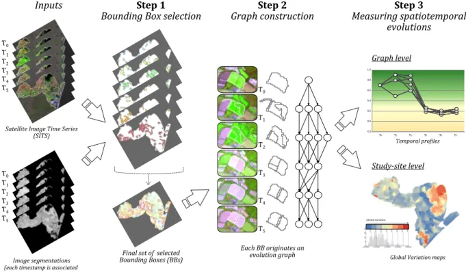
representation. The general framework of our methodology is summarized in Figure 1. 99
Inputs
Image segmentations
(each timestamp is associated to an independent set of objects)
Satellite Image Time Series (SITS)
Final set of selected Bounding Boxes (BBs)
Each BB originates an evolution graph
Study-site level Graph level
Global Variation maps Temporal pro�iles
Step 1
Bounding Box selection Graph constructionStep 2 Measuring spatiotemporalStep 3 evolutions T0 T1 T2 T3 T4 T5 T0 T1 T2 T3 T4 T5 Global variation -0,2 0,0 0,2 0,4 0,6 0,8 1,0 139 112 122 106 140 141 135 134 136 129 133 144 125 131 139 135 141 T0 T1 T2 T3 T4 T5 T0 T1 T2 T3 T4 T5
Figure 1: General framework showing the main steps of the methodology.
Given a SITS data and its associated segmentation, firstly we select a set of objects 100
that represent the spatial entities we want to monitor during the time. We call such subset 101
of objects Bounding Boxes (BBs). The set of BBs can contain objects coming from any 102
timestamp. The term spatial entities is used in this paper to designate a part (any portion) 103
of a given study site. Then, for each Bounding Box (BB ), we create an evolution graph con-104
sidering all the objects, in all the timestamps, that are covered by the BB area. Each vertex 105
of a graph corresponds to an object. Two vertices are linked by an edge if they belong to 106
two successive timestamps and the corresponding objects overlap each other.The procedure 107
is applied to each BB and the result consists in a set of evolution graphs summarizing the 108
different spatiotemporal phenomena existing in the study site. The set of evolution graphs 109
is successively exploited, with the object related information (e.g. spectral, geometrical, tex-110
tural, etc.) in order to supply analysis at graph and study-site levels. The first level allows 111
namely the analysis of the temporal trajectories (or profiles) of a particular spatiotempo-112
ral phenomenon while the second level supplies a more general picture summarizing the 113
temporal dynamics detected over the entire study site. 114
2.2. Bounding Box selection 115
The first step of our process consists in the selection of coherent BBs (i.e. spatial entities) 116
to monitor along the different timestamps. This operation analyzes all the objects provided 117
by the input segmentations (all the timestamps) and selects a subset of different spatial 118
entities covering as much as possible the whole study site. To deal with this task we made 119
some assumptions that are justified from the nature of the SITS data we manage. 120
The first assumption we made is related to the fact that each selected BB has, during 121
the period considered by the SITS, a maximal extent (or footprint) from a spatial point 122
of view. For instance, if we consider a temporary lake, in the time series we will have a 123
timestamp in which it reaches its maximal spatial extent while for the other timestamps 124
the same area may be segmented in different objects as water will cover a less important 125
area. In our approach we attempt to select maximal footprints as BBs. To select the set 126
of BBs, we adopted the following strategy: first we select a subset of the objects respecting 127
the assumption on the maximal footprint, we named such set of objects candidateBB. Then, 128
from candidateBB we filtered out a subset of objects that cover as much as possible the 129
study site and that overlay as less as possible between each other from a spatial point of 130
view. 131
Since all the images span over the same grid of pixels, we can retrieve for each pixel of 132
each timestamp the object it belongs to and therefore select the largest one. The process 133
is repeated over the whole study site and the selected objects are added to candidateBB. 134
This pre-selection explicitly implements the maximal footprints assumption over the whole 135
study site. However, this process may retain objects representing very similar geographical 136
areas. To deal with this redundancy issue we designed an algorithm that, starting from 137
candidateBB, selects a set of objects to minimize as much as possible the degree of overlay. 138
More in detail, the algorithm iterates over the set of candidateBB until no more objects 139
can be included in the final set of BBs. At the beginning, the set of BBs is initialized to 140
the empty set. A data structure containing the grid pixels covered during the process is 141
initialized with the empty set. We call this structure PAC (Pixel Already Covered). At 142
each iteration, the more promising object is selected from the candidateBB and added to 143
the final set of BBs. The more promising object is determined considering the following 144 piecewise function (1): 145 weight(O) = size(O) if novelty(O) = 1 novelty(O) if α ≤ novelty(O) < 1 0 if novelty(O) < α (1) where: 146
• size(O) is the size of the object, in this case the number of pixels 147
• novelty(O) is the contribution of the object w.r.t. the current partial solution 148
• α is a threshold parameter defining the minimum value of novelty an object must show 149
to be added to the final set of BBs 150
1. 151
More in detail, the novelty numerically describes the contribution of each object (belonging 152
to candidateBB ) w.r.t. the partial solution achieved by the procedure. The novelty is defined 153
as follows (2): 154
novelty(O) = |size(O) − P AC(O)|
size(O) (2)
where: 155
• size(O) = the number of pixels of the object 156
• P AC(O) = the number of pixels already covered by the current partial solution for a 157
given object 158
In summary, the weight assigned to each candidateBB object is dynamically recomputed 159
during the procedure. This is done because we update the PAC variable whenever an object 160
is added to the final set of BBs. According to the weight(O) function, first we will select all 161
the bigger and non-overlapping objects from candidateBB as their novelty value is equal to 162
1. Then, we will start to select the objects presenting the higher novelty values in order to fill 163
the remaining uncovered areas of the study site. The process stops when all the remaining 164
candidateBB objects present novelty values lower than the parameter α or all the grid pixels 165
of the study site are covered. The value of α is inversely proportional to the number of BBs 166
in the final set. High values of α will lead the selection of a small set of BBs, while small 167
values of α will allow the procedure to extract a bigger set of BBs. Another point we can 168
stress on is that the BBs extracted with a big value of α (e.g. 0.5) will be a subset of the 169
BBs extracted with a small value of α (e.g. 0.3). This is due to the fact that the proposed 170
procedure is deterministic and has a monotonic behavior. Decreasing the value of α will 171
relax the spatial overlay constraint going further in the selection process. 172
2.3. Graph construction 173
The final set of BBs defines the spatial entities (and their related phenomena)we will 174
monitor throughout the SITS. Logically, each BB has a unique spatial extent (footprint) 175
which is used to select and link the objects from one timestamp to the next one. Given 176
a BB, we project its footprint over each timestamp of the time series and we select the 177
objects overlapping with BB. In order to avoid the selection of non-representative objects 178
(or parasite objects) w.r.t. the area we monitor, we established two parameters that can 179
be translated to the following restrictive conditions: (a) at least τ1 of the object should be
180
inside of the BB footprint, (b) the object should represent at least τ2 of the BB footprint
181
where both τ1 and τ2 are two percentages.The first parameter (τ1) is the most important
and control the selection of objects that should present most of their spatial extent outside 183
the BB footprint. The second parameter (τ2) is used to keep all the objects filling more
184
than a certain percentage of the BB footprint, irrespective of any other statement. 185
After this selection, each BB will be associated to a set of objects which can be organized 186
and stored as an evolution graph. The graph is built linking the objects of timestamp i with 187
the objects of timestamp i + 1. Each object corresponds to a vertex of a graph and the 188
weight of the link (edge) represents the degree of overlap between two objects. In this way 189
we obtain graphs that have as many layers as the number of images in the time series. 190
Another intrinsic characteristic of an evolution graph is that, for a certain layer, it will 191
contain only one object (corresponding to the BB ). Logically, objects belonging to the same 192
timestamp are not connected; this is also true for objects not belonging to two successive 193
timestamps. In other words, the graphs created by our procedure are oriented graphs, more 194
precisely temporal oriented graphs. An oriented graph is the same thing as a loopless simple 195
directed graphs (West, 2001), also called Directed Acyclic Graphs (DAGs) (Maurer, 2003). 196
2.4. Computing graph coverages 197
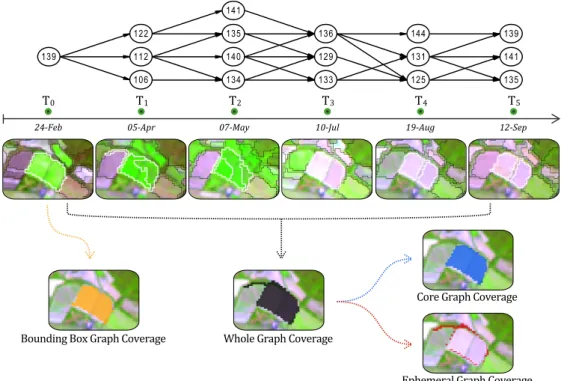
Each evolution graph is associated to an unique BB and can be represented by several 198
spatial coverages (see Figure 2). The simplest way is to use the spatial extent of the former 199
BB to represent the graph (e.g. in a map). We named this representation the Bound-200
ing Box Graph Coverage (BBCov ). In order to get a Whole Graph Coverage (WholeCov ) 201
we calculated the total spatial extent of all the objects contained in the graph at all the 202
timestamps. The WholeCov can be decomposed in two components, the Ephemeral Graph 203
Coverage (EphemCov ) which groups the area(s) covered only once during the time series 204
and the Core Graph Coverage (CoreCov ) which indicates the area(s) covered at least twice 205
during the time series. Such surfaces (EphemCov and CoreCov ) can be expressed as per-206
centages of the WholeCov. High percentages of EphemCov indicate unstable boundaries of 207
the graph objects and can be related to transitory evolutions in the study area. However, 208
sometimes this behavior can be produced by unsuitable segmentation results, e.g. under seg-209
mentation. In such a case the input segmentation can influence the extraction of interesting 210
evolution graphs. This means that the EphemCov value can be employed as an indicator 211
to estimate the quality of the time series segmentation and suggest, if necessary, to provide 212
a better input segmentation that will impact positively the graph coverage results. How to 213
optimize and produce coherent individual segmentations from a SITS is out of the scope of 214
this work since, these two elements (SITS and segmentations) are the inputs of the proposed 215
methodology. CoreCov usually encompasses the whole surface of the BBCov as well as a 216
buffer area around it. A big discrepancy between CoreCov and BBCov usually indicates 217
that the BB does not provide a good spatial representation of the whole graph. 218
In the example showed in Figure 2, the BB used to create the evolution graph comes 219
from the first timestamp (T0) and its coverage (BBCov ) is highlighted in orange color.
220
It represents two agricultural parcels covered by the same type of crop. In the following 221
timestamps, the number of objects ranged from 3 to 4 and the evolution graph totaled 222
17 objects. The union of all these objects corresponds to the WholeCov which is showed 223
in black. We can notice an elongation in the upper left part of the WholeCov polygon if 224
139 112 122 106 140 141 135 134 141 139 135 129 136 133 131 144 125
24-Feb 05-Apr 07-May 10-Jul 19-Aug 12-Sep
T0 T1 T2 T3 T4 T5
Whole Graph Coverage Bounding Box Graph Coverage
Core Graph Coverage
Ephemeral Graph Coverage
Figure 2: Example of an evolution graph extracted from a crop area. Graph nodes and edges are showed in the upper part, while the object boundaries (at each timestamp) are displayed below the timeline. The four types of spatial coverages computed for this evolution graph can be visualized in the bottom part of the figure.
compared to BBCov. The elongation does not correspond to the agricultural parcels targeted 225
by the BB but to a parasite object coming from T1. This undesirable inclusion is clearly
226
visible in the EphemCov (red color) which highlights also other small border sections around 227
the agricultural parcels. In this example, the CoreCov (blue color) is very similar to the 228
BBCov as the borders of the targeted parcels remained substantially stables during the time 229
series. 230
2.5. Measuring spatiotemporal evolutions at Graph and Study-site levels 231
In order to analyze and understand the information behind the evolution graphs, we 232
defined two levels of analysis: (a) the graph level and (b) the study-site level. In the former, 233
the focus is mainly on how the objects of the graph are linked (graph structure) and how 234
their attributes (content) evolve in time. In the latter, the focus is related to the whole 235
study site and especially on how the most stable and the most dynamic spatial entities are 236
distributed. 237
Considering the graph level analysis, given a graph G, we indicate with Gi the set of
238
objects covered by G at the timestamp i and with wj,k the weight of the link between object
239
oj and object ok. We compute the Variation (V ar) between two consecutive timestamps
240
with the following formula (3): 241
V ar(Gi, Gi+1) = X oj∈Gi size(oj) size(Gi) · P ok∈Gi+1wj,k· dist(oj, ok) P kwj,k (3)
The first part of the V ar formula is proportional to the importance of the object oj over
242
the set of objects at timestamp i. Therefore, size(oj) corresponds to the number of pixels of
243
oj while size(Gi) represents the total number of pixels covered by the graph G at timestamp
244
i. The second part of the formula evaluates the evolution between an object at timestamp i 245
w.r.t. the objects at timestamp i + 1 linked to it. In particular, the variation between two 246
timestamps is measured by a weighted sum of the euclidean distances between the attributes 247
of the object oj and ok. The weight wj,k quantifies the strength of the interaction between
248
oj and ok in terms of spatial overlay.
249
The Global Variation (GlobaV ar) for a graph is obtained cumulating the contribution 250
of each pair of consecutive timestamps as follows (4): 251 GlobalV ar(G) = n−1 X i=1 V ar(Gi, Gi+1) (4)
The GlobalV ar associated to an evolution graph estimates how much the area represented 252
by this graph evolves during the period covered by the time series. Potentially, this score can 253
vary between 0 and +∞.A low value of GlobalVar implies stable temporal behavior while a 254
high value indicates important temporal evolution throughout the time series. 255
Another option to perform graph-level analysis is by means of Temporal Profiles where 256
the temporal variation of any object attribute can be plotted for all the nodes of a given 257
graph. Temporal Profiles allow a more fine analysis of the graphs, facilitating the visualiza-258
tion and interpretation of temporal behaviors related to the graphs’ underling spatiotemporal 259
phenomena. More in detail, given a graph G and an attribute we want to monitor (e.g. the 260
NDVI), we can build a plot where the X-axis (resp. the Y-axis) represents the time (resp. 261
the attribute to study, i.e. NDVI). Such plot will contain the objects of the graph temporally 262
arranged from the first to the last timestamp. Such a representation combines the graph 263
structure and the content (i.e. the attribute chosen to perform the analysis), allowing to 264
follow the evolution of these elements conjointly all over the SITS. Examples of Temporal 265
Profiles are reported in the experimental results (see Figure 8). 266
Considering the study-site level analysis, the GlobalV ar scores (computed for each evo-267
lution graph) can be used to produce a GlobalVar map. In this kind of representation, any of 268
the computed graph coverages (e.g. CoreCov ) can be used to construct the map. According 269
to the selected coverage, the polygons representing the graphs will be colored following a 270
gradient proportional to their GlobalV ar scores. The GlobalVar map summarizes the distri-271
bution of the different phenomena detected within the study site and provides information 272
related to the intensity of the evolutions during the time. This kind of map, computed 273
automatically and considering the whole SITS, is an useful tool for exploratory researches 274
over areas where the spatiotemporal dynamics are unknown (or few studied). GlobalVar 275
maps can also provide valuable information for planning field-campaigns and prioritizing 276
the visits over such unknown or few studied areas. In the case of similar temporal sampling, 277
GlobalVar maps may be used to compared the spatiotemporal dynamics of two (or more) 278
different study sites. 279
While the Temporal Profiles are more suitable for analyzing one particular object at-280
tribute at time, GlobalV ar scores (and maps) can be also obtained considering all the 281
attributes or a subset of them (e.g. only a few spectral indices or a given combination of 282
spectral bands). 283
It is important to highlight that the GlobalVar score is more suitable for short-term 284
landscape analysis (e.g. intra-annual scale) and less appropriate for long-term landscape 285
evolution monitoring (e.g. multi-annual scale) since different temporal trajectories can col-286
lapse to the same score value. Conversely, the information supplied by Temporal Profiles can 287
be adopted to study both short-term or long-term landscape evolutions since it preserves 288
the full temporal trajectories associated to an evolution graph. 289
2.6. Parameter Setting 290
As previously noticed, our methodology needs the setting of three different parameters: 291
α, τ1 and τ2. The first parameter limits the overlay among the selected BBs while the
re-292
maining two parameters avoid the selection of non-representative objects in the construction 293
of the evolution graphs. 294
With the aim to facilitate the choice of these parameter values, we propose to consider 295
the coverage and the redundancy of the extracted evolution graphs. The coverage of the 296
evolution graphs is the union of the WholeCov of each of the graphs in the solution. This 297
measure quantifies how much of the study site is covered by the selected graphs. Concerning 298
the redundancy in the set of extracted graphs, we evaluate this quantity as the portion of 299
the study site that is covered, at least, by two different graphs. This quantity measures how 300
much redundancy exists in the obtained solution. 301
In order to determine the three initial parameters (and the corresponding set of evolution 302
graphs), we firstly generate different solutions varying the α, τ1 and τ2 parameters and then,
303
we fix a threshold (σ) that defines the minimum accepted coverage. The σ threshold is 304
expressed as a percentage of the whole study area. Once the threshold σ is fixed, we obtain 305
a set of solutions that meets this constraint. Among such set of solutions, we choose the one 306
with the minimum redundancy value. We remind that this analysis can be performed in a 307
completely unsupervised way, independently from a possible ground truth data associated 308
to the SITS. 309
3. Case study 310
3.1. Data and Study sites 311
3.1.1. Time series data 312
We used Landsat-5 TM and Landsat-7 ETM+ level-2A products available through the 313
THEIA Data Centre (France). Such images were already ortho-rectified and corrected from 314
atmospheric, environmental and slope effects as described by Hagolle et al. (2010). Each 315
Landsat product was composed by six spectral bands (approximate center in nm): blue (485), 316
green (565), red (665), NIR (820), SWIR-1 (1650) and SWIR-2 (2190). With a pixel size of 317
30 m, the raster data is expressed in surface reflectance. We selected six Landsat cloud-free 318
images covering two study sites (described latter) between February and September 2009 319
(see Table 1). 320
Timestamp Acquisition date
T0 24 Feb. 2009 T1 05 April 2009 T2 07 May 2009 T3 10 July 2009 T4 19 Aug. 2009 T5 12 Sept. 2009
Table 1: Acquisition date of the selected Landsat images over the South of France.
The selected time series spreads from the end of the winter up to the end of the summer. 321
Such temporal range encompasses the entire growing season for natural vegetation as well 322
as the main agricultural cycles over the study sites. 323
3.1.2. Study sites description 324
Two sites were selected in the south of France, close to the Mediterranean Sea. Figure 325
3 presents the spatial boundaries of the two sites: (A) Libron Valley and (B) Lower Aude 326
Valley Natura 2000 site. Both sites are located inside the extent of the Landsat scenes 327
composing our time series. Figure 4 shows the study areas at each timestamp. 328
Located less than 10 km northeast from the city of B´eziers (France), the Libron Valley
329
site is mainly composed by agricultural parcels and natural areas. The site has about
330
1 655 ha and is crossed by the small coastal river named Libron. Agricultural parcels are 331
concentrated principally along the Libron waterway. Cereal crops dominate its upstream 332
section (northwest of the site) while the downstream section is mainly occupied by vineyards 333
(southeast of the site). The natural areas are essentially composed by patches of forest 334
(mainly coniferous) and scrubland. Most of these patches are in the north of the Libron 335
River, some of them encircle a golf field situated in the northern part of the site. In a 336
general way, the limits between agricultural and natural areas over this site can be easily 337
recognized in the Landsat images. Such a task is possible because agricultural parcels and 338
forest patches are usually bigger than 6-8 ha (i.e. 200 m x 400 m or wider for most of the 339
crop fields). 340
The Lower Aude Valley is a Natura 2000 site located in the terminal section of the Aude 341
River. Before reaching the Mediterranean Sea, the Aude River crosses a flat wetland area of 342
about 4 842 ha. From a biodiversity point of view, 56.3% of the site is composed of natural 343
habitat types of Community interest (NHCI). In total, 19 NHCI are part of the site, including 344
5 priority habitat types. The most widespread habitats are: Mediterranean saltmarshes and 345
Saline coastal lagoons. The remaining area (43.7%) is principally occupied by vineyards, 346
cereal crops and temporary or permanent meadows. In opposition to the Libron site, the 347
agricultural parcels are often small within this site (usually around 1-2 ha) and therefore 348
more difficult to identify using Landsat images. Another particularity, the site is exposed to 349
BEZIERS Mediterranean Sea Aude
B
A
km 0 5 10 Orb Libron F. Güttler (2012) 3°05'00" E 43°23'06" N 3°25'32" E 43°11'00" NFigure 3: Location and boundaries of the selected study sites (A Libron Valley ; B Lower Aude Valley Natura 2000 site).
J F M A M J J A S O N D
Landsat Time Series 2009
24-Feb 05-Apr 07-May 10-Jul 19-Aug 12-Sep
24-Feb 05-Apr 07-May 10-Jul 19-Aug 12-Sep
AA
BB
Figure 4: Time series for the selected study sites (A Libron Valley ; B Lower Aude Valley Natura 2000 site) during 2009.
flooding events (mostly during winter) as well as to drought episodes (maximum intensity 350
occurring in the end of the summer). The flooding areas are situated predominantly around 351
the two coastal lagoons: Vendres in the north part of the site and Pisse-Vaches in the south. 352
The Mediterranean Sea has also an influence over the salinity across the site (soils and water 353
bodies), with a general gradient increasing from northwest to southeast. 354
3.2. Preprocessing and segmentation 355
3.2.1. Spatial subset and fine geometrical registration 356
Although level 2-A products were already ortho-rectified, we observed some spatial im-357
precision when overlapping all the time series images. For this reason, additional fine spatial 358
positioning corrections were necessary in order to keep the spatial shift between any times-359
tamp less than a pixel. Afterwards, two spatial subsets (one for each study area) were 360
performed over each Landsat image. 361
3.2.2. Spectral indices 362
Spectral indices are commonly used in remote sensing as they can be helpful for detect-363
ing and characterizing some specific features, like vegetation, soil, water, etc. In this work 364
we calculated three spectral indices compatible with Landsat data using the formula pro-365
vided by the literature: a) Normalized Difference Vegetation Index NDVI (Rouse Jr et al., 366
1974); b) Normalized Difference Water Index NDWI (Gao, 1996); c) Visible and Shortwave 367
Infrared Drought Index VSDI (Zhang et al., 2013). NDVI is sensitive to the amount of 368
photosynthetically active vegetation present in the plant canopy (Tucker, 1979) and has 369
been extensively used in remote sensing applications since the 1970s. NDWI is sensitive to 370
changes in liquid water content of vegetation canopies (Gao, 1996) and has been used to 371
estimate vegetation water content (Jackson et al., 2004). VSDI is sensitive to changes in 372
soil and vegetation moisture and was conceived to monitor drought over different types of 373
land cover during plant-growing season (Zhang et al., 2013). 374
3.2.3. Time series image segmentation 375
Image segmentation is a fundamental step in OBIA and it consists in merging pixels into 376
object clusters (Baatz et al., 2008). Objects (or segments) are regions generated by one or 377
more criteria of homogeneity in one or more dimensions of a feature space (Blaschke, 2010). 378
The principal aim of segmentation is to create a new representation of the image, more 379
meaningful and easier to analyze. This approach is similar to human visual interpretation 380
of digital images, which works at multiple scales and uses color, shape, size, texture, pattern 381
and context information (Lillesand et al., 2008). Image segmentation results in a set of 382
objects that collectively cover the entire image without any overlapping. With respect to 383
the homogeneity criteria, adjacent objects are expected to be significantly different between 384
them. 385
In this work, image segmentation was performed with the Multiresolution Segmenta-386
tion Algorithm (MSA) 1. We choose the MSA algorithm instead of recent approaches based
387
on superpixel Achanta et al. (2012) since the objective of our strategy is to capture phe-388
nomena that can lie at different scales. Adopting a superpixel segmentation method, like 389
SLIC (Achanta et al., 2012), will produce segments at equal scale and this will be in con-390
trast with the main assumption of our work (maximal spatial extent detection). Conversely, 391
the MSA scale parameter is intrinsically related to the homogeneity criterion which takes 392
into account both shape and radiometry of objects in a combined manner. For this reason, 393
over two areas of the same size, MSA may provide multiple small objects if the target is 394
heterogeneous or, a single larger object if the target is more uniform. 395
Only the pixels within the boundaries of the study sites were used during the segmen-396
tations. Nine raster layers were simultaneously used for image segmentation. Six of them 397
correspond to the Landsat spectral bands and the other three to the spectral indices. In 398
order to obtain objects representing the natural and agricultural boundaries over the study 399
sites, we conceived a segmentation rule-set composed of 3 main steps as showed in Figure 400
5. For simplification purposes only the Lower Aude Valley site is presented in this figure 401
as well as in the subsequent explanations. However, the same rule-set was applied over the 402
Libron Valley site. 403
step1. medium-coarse segmentation
(180 objects at T )0 0
step2. very �ine segmentation
(5595 objects at T )
step3. �inal segmentation
(514 objects at T )0
Figure 5: Segmentation rule-set outputs (at T0) for the Lower Aude Valley Natura 2000 site. The first step delimits the general zones trough a medium-coarse segmentation. MSA 404
was configured here to combine both color and shape components but using predominantly 405
color (0.8). About 170-200 objects are obtained per timestamp over the Lower Aude Valley 406
site. In the second step, a very fine segmentation is performed inside the object boundaries 407
created at step 1. Focused exclusively on the color component, it creates about 6 000 objects 408
per timestamp. In step 3, medium-fine segmentation is performed taking into account the 409
results of the previous steps. With balanced weights for color and shape components, step 3 410
segmentation creates about 500-600 objects per timestamp. The segmentation rule-set was 411
executed for each timestamp separately. In other words, the set of objects obtained at T0
412
does not impact the segmentation process at T1 and so on. The segmentations were also
413
separately performed over each study site. For both sites and timestamps, only the objects 414
obtained at the last level of segmentation (step 3) were exported and used as an input for 415
the subsequent processing steps. 416
3.3. Verification strategies 417
To assess the quality and the accuracy of the results, we developed two verification 418
strategies. The first was based on the interpretation of the ancillary imagery plus two 419
thematic layers and was applied over the Lower Aude Valley site. The second strategy was 420
mainly based on the official farmer declarations (one of the available thematic layer) and 421
applied over the Libron Valley site. 422
Considering the ancillary imagery, two types of image were employed: (a) normal color 423
and color infrared aerial orthophotos (0.5 m spatial resolution) acquired during May 2009 424
and (b) one RapidEye satellite image (6.5 m spatial resolution) acquired in 24 June 2009 425
and only available for the Lower Aude Valley site. 426
Regarding the thematic layers, the first concerns both study areas and is related to 427
agricultural practices. It corresponds to the official farmer declarations indicating the main 428
cultures exploited during 2009. The second thematic layer is proper to the Lower Aude 429
Valley site. It corresponds to a detailed classification (scale 1:25 000) of the natural habitats 430
over the site. The classification was realized by botanists and ecologists of the Conservatory 431
for the Natural Spaces of the Languedoc-Roussillon Region (CEN-LR). 432
3.3.1. Ancillary imagery based verification 433
First, the aerial photographs were used to map the whole Lower Aude Valley Natura 434
2000 site. This task was carried out through a manual land cover digitalization process 435
at the 1:10,000 scale. Each individual map unit (polygons in our case) has been labeled 436
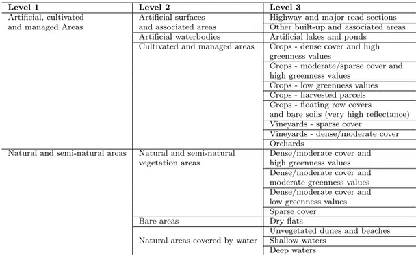
according to hierarchically structured land cover classes. This hierarchy contains three levels 437
of complexity and has, in the more detailed level (3), nineteen land cover classes. Eleven 438
of them are associated to artificial, cultivated and managed areas, while the other eight 439
classes are related to natural and semi-natural areas (see Table 2 for all the class names). 440
Considering the acquisition date of the aerial photographs, the obtained land cover map 441
represents the situation of the site in May 2009. 442
Then, the obtained land cover map was superimposed on the RapidEye satellite im-443
age. All the initial polygons received a new land cover label (using the same hierarchical 444
scheme) according to the situation observed on the RapidEye image (24th June 2009). 445
When necessary, new boundaries were digitalized and some polygons of the former map 446
were consequently divided into two or more smaller polygons. Thus, a second land cover 447
map was produced representing the situation of site in late June 2009. In order to estimate 448
the evolutions between the two land cover maps we computed an exhaustive set of from-to 449
evolution classes. Then, we analyzed each from-to evolution class (about 50) and assigned 450
a particular level (or intensity) of change: low, medium, high or very high. Finally, these 451
Level 1 Level 2 Level 3
Artificial, cultivated Artificial surfaces Highway and major road sections
and managed Areas and associated areas Other built-up and associated areas
Artificial waterbodies Artificial lakes and ponds
Cultivated and managed areas Crops - dense cover and high
greenness values
Crops - moderate/sparse cover and high greenness values
Crops - low greenness values Crops - harvested parcels Crops - floating row covers
and bare soils (very high reflectance) Vineyards - sparse cover
Vineyards - dense/moderate cover Orchards
Natural and semi-natural areas Natural and semi-natural Dense/moderate cover and
vegetation areas high greenness values
Dense/moderate cover and moderate greenness values Dense/moderate cover and low greenness values Sparse cover
Bare areas Dry flats
Unvegetated dunes and beaches
Natural areas covered by water Shallow waters
Deep waters
Table 2: Hierarchically structured land cover classes used for mapping the Lower Aude Valley site. This scheme was used to create two maps, one derived from the aerial photographs and the other from a RapidEye image.
intensities of change (derived from the ancillary imagery) were compared to the GlobalVar 452
scores, obtained from the evolution graphs (described in Section 2.5). 453
3.3.2. Thematic layer based verification (official farmer declarations) 454
The second verification procedure consisted in drawing up a parallel between the Global 455
Variation results and the principal groups of culture declared annually by the farmers. In 456
France, the reference parcel representation is the Farmers block/ilot in regard to the Euro-457
pean regulation (Comm. Reg. N 796/2004 ). This kind of parcel representation corresponds 458
to an association of one or more agricultural parcels into blocks. Each block is the property 459
of a single farmer and may contain one or several crop groups (Sagris and Devos, 2008). In 460
practice, the official farmer declarations (the public version of the data) consists in a set 461
of georeferenced polygons (one for each block) were a code indicates the principal groups 462
of culture exploited during the year. Within the Libron Valley site, 11 groups of culture 463
have been declared in 2009 which corresponds to 59 polygons. Nevertheless, this thematic 464
layer contains some erroneous declarations, imprecise polygon boundaries and some gaps 465
(i.e. when an agricultural parcel has not been declared). In order to attain a more precise 466
comparison, we verified each polygon and selected only those without visible errors. Also, 467
we eliminated all the polygons smaller than 4 ha to preserve an order of magnitute compa-468
rable with the graph objects. The obtained subset contains 32 polygons belonging to the 469
following groups of culture: cereals (excepted wheat), flower-fruit vegetables, orchard, seeds, 470
sunflower and vineyard. As these cultures are associated to dissimilar agricultural practices 471
Lower Aude Valley Libron Valley
Min Mean Max Min Mean Max
Number of nodes 7 15.2 38 6 13.0 26 Number of edges 7 24.5 77 5 18.9 53 Number of paths 2 79.7 1050 1 46.7 480 BBCov (ha) 1.6 16.2 125.0 3.2 13.8 67.1 WholeCov (ha) 5.3 46.2 175.7 6.1 34.5 107.9 CoreCov (ha) 2.1 29.9 142.5 3.4 22.6 94.6 CoreCov (%) 13.9 65.1 90.9 14.4 66.3 93.3 EphemCov (ha) 0.8 16.4 134.0 1.2 11.8 65.1 EphemCov (%) 9.1 34.9 86.1 6.7 33.7 85.6
Table 3: Global graph statistics obtained for each study site
and temporal dynamics all along the year, it is expected some noticeable differences among 472
the graphs representing these areas (especially w.r.t. the GlobalVar results). 473
4. Experimental Results and Discussion 474
4.1. Overall results and statistics 475
To generate the evolution graphs on the two study sites we used the procedure introduced 476
in Section 2.6. We fixed the σ threshold (the minimum accepted coverage) equals to 95% 477
and generated the set of different solutions varying the three parameters (α, τ1 and τ2) in
478
the range [0.1, 1] with a step-size of 0.05. The procedure selected the following values for α, 479
τ1 and τ2: 0.3, 0.25 and 0.20 respectively. The values are the same for both sites.
480
We obtained a total of 340 graphs for the Lower Aude Valley site and a total of 142 481
graphs for the Libron Valley site. The total number of objects per graph ranges from 6 (a 482
single object per timestamp) to 38 (about 6.3 objects per timestamp). The mean value, 483
considering both study sites, was 14.6 (about 2.4 objects per timestamp). Also considering 484
the two study sites, the mean number of edges per graph was 22.9 while the mean number 485
of paths per graph was 69.9. Taking into account all the 482 graphs, the whole spatial 486
coverages (WholeCov ) ranges from 5.3 ha to 175.7 ha with a mean value of 42.7 ha. Although 487
some graphs present very high coverages (>100 ha), most of the values (about 97%) range 488
between 10 and 90 ha. In other words, the areas monitored by our graphs correspond mostly 489
to patches ranging from 100 to 1000 Landsat pixels. As another global result, the core graph 490
coverages (CoreCov ) correspond, in average, to 65.5% of the WholeCov areas. As expected, 491
EphemCov is usually smaller than CoreCov and this is true for 87.5% of the graphs. Even if 492
all the processing steps were identical for the two study sites, we noticed some differences in 493
the graph derived statistics. Table 3 shows the main statistical results obtained separately 494
for each study site. 495
We can observe that the Lower Aude Valley graphs have a bigger number of nodes if 496
compared to those of the Libron site. In general, they tend to present a more complex 497
structure with a higher number of paths per graph. Another noticeable difference is related 498
to the size of the objects and the derived graph coverages. All the greatest objects (>70 ha) 499
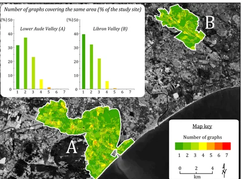
Number of graphs 1 2 3 4 5 6 7 0 2 4 km
A
B
(%) (%)Number of graphs covering the same area (% of the study site)
Map key Libron Valley (B)
Lower Aude Valley (A)
0 10 20 30 40 50 1 2 3 4 5 6 7 0 10 20 30 40 50 1 2 3 4 5 6 7
Figure 6: Degree of spatial overlapping among graphs for both study sites. The histogram indicates the relative areas (% of each study site) considering number of graphs covering the same area.
comes from the Lower Aude Valley as well as most of the widest graphs (>100 ha w.r.t. the 500
WholeCov ). This can be explained by the exclusive presence of water bodies and temporally 501
flooded areas in the Lower Aude Valley site. The spectral homogeneity of these particular 502
areas contributes to generate large objects during the image segmentation step. 503
As the graph coverages may partially overlap, it becomes interesting to detect the spatial 504
distribution of the less and most overlapping areas. Figure 6 shows such spatial distribution, 505
in terms of number of graphs representing the same area, over the two study sites. The spatial 506
overlapping is related to the value of the parameter α (novelty threshold) used during the BB 507
selection strategy presented in Section 2.2. This threshold allows a certain level of overlay 508
among the BBs, it is expected that all the other derived graph coverages will present some 509
degree of overlap as well. As a consequence, the higher is the α parameter, the lower will 510
be the number of selected BBs, the lower will be the degree of spatial overlapping among 511
the generated graphs. On both study sites we have observed that, when α is lower than 0.2 512
the degree of overlay becomes particularly high (more than 75% of the study site is covered 513
by two or more graphs) while α values larger than 0.4 lead to important gaps (areas not 514
covered by any graph). 515
However, the spatial overlapping depends also on the inner characteristics of each study 516
site, in particular on how the spatial boundaries of their objects evolve during the time 517
series. In the case of our study sites, the Libron Valley presented a lower degree of spatial 518
overlapping w.r.t. the Lower Aude Valley. This can be explained by two main factors: (a) 519
the spatial arrangement of the sites, e.g. in the Libron site the limits between agricultural 520
and natural areas are easier to recognize (bigger and more homogeneous patches) and (b) 521
nature of the temporal evolutions, e.g. modifications in the shape of the objects are more 522
frequent in the Lower Aude Valley since the site is exposed to flooding events. In addition, 523
the fact of having many small parcels (near to the limit of detection) may contribute to 524
shape instability from a timestamp to the next one. 525
4.2. Spatiotemporal Dynamics 526
When repeatability and compatibility of satellite observations are guaranteed it becomes 527
possible to detect spatiotemporal evolutions, from which the related dynamics can be de-528
duced (Bonn, 1996). In that light, we consider spatiotemporal dynamics as derived from 529
a set of consecutive evolutions we detected throughout the time series. In particular, we 530
performed analysis at both graph and study-site levels (as described in Section 2.5). 531
4.2.1. Graph Level Analysis 532
In order to better illustrate graph structure and content, we selected 4 graphs represent-533
ing different evolutions in time (see Figure 7). Graph A represents a natural area composed 534
mainly by scrubland and forest. Its BB came from the fourth timestamp which corresponds 535
to the beginning of the summer. At this time, the area is the most homogeneous while the 536
most heterogeneous situations are observed in the first (winter) and third (spring) times-537
tamps. In those two timestamps it is possible to better distinguish the deciduous vegetal 538
community (brown at T1 and light green at T3) from the surrounding coniferous community
539
(dark green during the whole time series). Conversely, Graph B has a particular structure 540
with two very distinct portions: first there is a single object per timestamp from T0 to T3
541
whereas from T4 to T5 there are several objects per timestamp (8 and 6 respectively). The
542
huge spatial fractioning observed between T3 and T4 corresponds to the drying-up process
543
of the Pisse-vaches coastal lagoon. High evaporation rates combined to weak precipitations 544
during the summer leads to the replacement of the lagoon by a wide dry salt flat in the end 545
of this season. Graph C presents a quite similar, but inverted, structure w.r.t. Graph B. In 546
fact, this saltmarsh and salt meadow area is more heterogeneous in the beginning of the time 547
series (T0 up to T2). At this time, the area is partially covered by water and hygrophilous
548
vegetation, which explains the dissimilarities on the objects boundaries during these three 549
timestamps. Afterwards, water is no more present and the dry summer conditions lead to 550
a fast decrease of the photosynthetic vegetation, as a consequence, the area becomes much 551
more homogeneous in the three last timestamps. Finally, Graph D represents the evolutions 552
over two adjacent cereal crop fields. The plant-growing season is visible from T0 to T2 (late
553
winter to spring) although we can notice that plant-growing is not homogeneous all over the 554
field area. Then, the crops are harvested in early summer (between T2 and T3) and both
555
fields remain unvegetated until the end of the time series. 556
In addition to graph structure and visual analysis of image objects, it is important to 557
consider the changes in the content of the objects. For that purpose, each graph can be 558
also finely analyzed thanks to Temporal Profiles representing the variation of any object 559
attribute. As examples, we can use the previously discussed graphs B and D (see Figure 8). 560
In the case of Graph B, the temporal behavior of VSDI furnishes reliable information about 561
the drying-up process of the coastal lagoon as this spectral index is sensitive to changes in soil 562
139 112 122 106 140 141 135 134 141 139 135 129 136 133 131 144 125 133 87 71 102 107 111 89 104 111 124 101 76 111 104 112 82 121 136 100 69 90 101 34 19 30 28 58 44 20 40 45 22 27 49 40 33 488 457 540 525 528 530 551 532 523 565 556 568 553 558 563 550 539 542
24-Feb 05-Apr 07-May 10-Jul 19-Aug 12-Sep
T0 T1 T2 T3 T4 T5
Graph D Graph C Graph B Graph A
= object used as Bounding Box during the graph contruction step
Figure 7: Examples of graphs showing different structures and representing distinct evolutions in time. A- a scrubland and forest area (central part of the Libron site), B- a coastal lagoon (southern part of the Lower Aude Valley), C- a saltmarsh area (northern part of the Lower Aude Valley), D- two crop fields (near to the central part of the Libron site).
-0,2 0,0 0,2 0,4 0,6 0,8
1,0NDVI temporal pro�ile
139 112 122 106 140 141 135 134 136 129 133 144 125 131 139 135 141 -350 -300 -250 -200 -150 -100 -50 0
50VSDI temporal pro�ile
488 457 540 565 523 551 530 528 525 532 563 553 558 542 568 539 550 556 139 112 122 106 140 141 135 134 141 139 135 129 136 133 131 144 125 488 457 540 525 528 530 551 532 523 565 556 568 553 558 563 550 539 542 Graph D Graph B T0 T1 T2 T3 T4 T5 T0 T1 T2 T3 T4 T5
Figure 8: Temporal profiles for two selected graphs (see 7). For Graph B (left) the temporal profile corre-sponds to the variation of the VSDI (each object is represented by its mean VSDI value) while for Graph D (right) it corresponds to the variation of the NDVI (each object is represented by its mean NDVI value).
moisture and to the presence of surface water. Likewise, for Graph D, the NDVI temporal 563
profile is useful to follow the changes observed over the cereal crop fields, i.e. plant-growing, 564
harvest and long-lasting bare soil. 565
4.2.2. Study-site Level Analysis 566
Beside such fine temporal information, the Global Variation (GlobalVar ) synthesizes 567
how much the area represented by a given graph evolves during the whole time series and a 568
GlobalVar map can be built from this information. Several GlobalVar maps can be produced 569
by combining different object attributes. Indeed, GlobalVar maps are useful to compare 570
graphs and promptly detect the most and the less stable areas within the considered study 571
sites. In our case, as both study sites have the same timestamps, GlobalVar maps can also 572
be used to compare the two zones (see Figure 9). 573
Regarding Figure 9, we can observe that choosing different attribute combinations results 574
in somewhat different GlobalVar maps. We can also underline that the two study sites 575
exhibit different behaviors considering different attribute combinations. In other words, the 576
attributes showed in Figure 9 are differently correlated according to each site and, in general, 577
they are not highly correlated among them. Regardless of the attribute selection, the Libron 578
site presents invariably higher values of GlobalVar if compared to the Lower Aude Valley. 579
This is more evident when only the NDVI is employed (map 1) or only the raw bands (map 580
2) to produce maps by means of GlobalVar, instead of map (3) where all the spectral indices 581
were used. 582
0 2 4 km
A
B
1
2
3
Global Variation maps over the two study sites (histograms represent the relative frequency for each site)
Libron Valley (B) Lower Aude Valley (A)
Lower Aude Valley (A)
Lower Aude Valley (A)
Libron Valley (B)
Libron Valley (B)
Results for Global Variation considering: 1 2 3 0 2 4 6 8 10 12 (frequency in %) - +
GlobalVar (all indices)
0 2 4 6 8 10 12 (frequency in %) - +
GlobalVar (all indices)
0 2 4 6 8 10 12 (frequency in %) - +
GlobalVar (all raw bands)
0 2 4 6 8 10 12 (frequency in %) - +
GlobalVar (all raw bands)
0 2 4 6 8 10 12 (frequency in %) - + GlobalVar (NDVI) 0 2 4 6 8 10 12 (frequency in %) - + GlobalVar (NDVI)
only the NDVI all the raw bands all the spectral indices
Figure 9: Global Variation (GlobalVar ) maps and the corresponding frequency histograms for the two study sites (A-Lower Aude Valley, B-Libron Valley). The following attributes were used for the GlobalVar maps: (1) only the NDVI, (2) all the raw bands and (3) all the spectral indices. As graph coverages may partially overlap, the GlobalVar values has been recalculated, for all the overlapping areas, considering the proportional contribution of the involved graphs.
Considering only the Lower Aude Valley, one can suppose a very stable situation based 583
on the analysis of the second map (all raw bands). Excepting few cereal crops in the western 584
part of the site, all the remaining areas present low values of GlobalVar, including all the 585
temporary flooded areas. Alone, the six spectral bands provide a very partial representation 586
of the temporal dynamics since only some radical evolutions (i.e. bare soil/dense vegeta-587
tion/bare soil) are highlighted, while the other evolutions are not took into account. Over 588
the Libron Valley site such kind of radical evolution is more frequent and widespread, espe-589
cially in the crop areas located along the upstream Libron waterway (red and orange hues 590
in map 2). However, even in this case the results are not satisfactory as some crops areas 591
presenting radical evolutions displays medium values of GlobalVar instead of high values. 592
Conversely, the GlobalVar map derived from the NDVI furnishes much more reliable 593
information related to landscape dynamics in both study sites. In the Libron Valley, the 594
highest values correspond to the agricultural areas where important changes are observed 595
throughout the year (e.g. cereals, sunflower, flower-fruit vegetables and seeds). Vineyards 596
and orchards generally experience less noticeable inter-annual variations and are therefore 597
assigned with medium or medium-low GlobalVar values. The lowest values correspond
598
mostly to natural scrub and forest areas, in particular those dominated by coniferous. In 599
the Lower Aude Valley, the lowest values are also principally related to natural areas, more 600
specifically to herbaceous/scrub vegetation covering sand dunes (southeast of the site) or 601
some not submerged areas surrounding the Vendres lagoon (center of the site). In addition, 602
some build-up areas like camping and recreational facilities (all located along to the coast) 603
present low GlobalVar values. Vineyards and orchards, as well as saltmarsh and salt meadow 604
areas, are generally assigned with medium or medium-low GlobalVar values. Finally, the 605
most dynamic areas are clearly associated to the two coastal lagoons (Vendres and Pisse-606
vaches) and, in a minor extent, to the few cereal crops located in the western part of the 607
site. The graphs representing the coastal lagoons and surrounding areas are characterized by 608
important changes in the objects shape and content. The Pisse-vaches sector is temporarily 609
covered by shallow and brackish waters. It is scarcely colonized by the vegetation either 610
during the submerged periods (very few aquatic macrophyte during winter and spring) either 611
during the waterless period (very limited growth of pioneer communities during the summer 612
and autumn). The Vendres sector also presents important seasonal water level fluctuations 613
but possess a permanently flooded area (northeastern portion). Salinity is less important 614
in this sector where dense aquatic and terrestrial vegetation can be observed during spring 615
and summer. 616
Finally, the third map of Figure 9 combines the three spectral indices to compute the 617
GlobalVar (all indices). The spatial distribution of the less and the most dynamic areas 618
is somehow similar to those described for the NDVI GlobalVar map, which is logical as 619
the NDVI is one of the three spectral indices considered here. Nevertheless, the inclusion 620
of VSDI and NDWI draw attention to some temporal evolutions unnoticed by the NDVI, 621
in particular over the areas where the contribution of the soil is greater than those of the 622
vegetation. 623
Pearson’s r Spearman’s rho
All raw bands 0.574 0.476
NDVI 0.767 0.659
NDWI 0.787 0.672
VSDI 0.719 0.580
All indices 0.789 0.676
Table 4: Correlation coefficients results for ancillary based verification. The value of change from ancillary imagery (VCA) was compared with five sets of GlobalVar (all raw bands, NDVI, NDWI, VSDI, all indices)
4.3. Ancillary imagery based verification 624
As explained in section 3.3.1, the ancillary imagery was processed in order to estimate 625
the intensities of change all over the Lower Aude Valley Natura 2000 site. Such intensities of 626
change were obtained by comparing two land cover maps and their related from-to evolution 627
classes. The first map (derived from aerial photographs) represented the study site in May 628
2009, while the second one (based on a RapidEye image) represented the site in late June 629
2009. This time interval corresponds roughly to the timestamps T2 (7 May 2009) and T3
630
(10 July 2009) of our Landsat time series. To perform a coherent verification, we calculated 631
an extra set the GlobalVar values considering only these two timestamps of the former time 632
series. 633
As the spatial boundaries between the evolution graphs and the land cover maps are not 634
similar, we employed the following strategy to compare their intensities of change. Starting 635
from the CoreCov of each graph, we clipped the corresponding polygon(s) of the land cover 636
maps. If a given graph is represented by more than one map polygon, we computed a 637
weighted average of the intensities of change of those polygons. This is done by taking 638
into account the relative area of each map polygon (inside the CoreCov ) and multiplying 639
it by a coefficient of change. The coefficient varies according to the intensities of change 640
(low=1, medium=2, high=3 and very high=4) assigned to the from-to evolution classes. As 641
consequence, each graph received a new numerical value of change (VCA) that is derived 642
from the ancillary imagery and can be therefore compared to the GlobalV ar values. 643
Table 4 summarizes the correlation coefficients obtained from the comparison of VCA 644
against five sets of GlobalV ar (all raw bands, NDVI, NDWI, VSDI, all indices). We used two 645
coefficients of correlation: (a) the Pearsons coefficient which measures the strength of the 646
association between two variables and (b) the Spearmans ranked coefficient which assumes 647
that the two variables under consideration were measured on an ordinal scale. 648
The strength of association is particularly high between VCA and three sets of GlobalVar 649
(all indices, NDWI and NDVI). This assertion is valid for the two correlation methods: 650
(a) Pearson’s r ranging from 0.767 to 0.789 and (b) Spearman’s rho ranging from 0.659 to 651
0.676. For both Pearson and Spearman, the correlation coefficient is very highly significantly 652
different from zero (p-value <0.0001). 653
It is worth noting that we eliminated the areas with potential water level fluctuations 654
from this comparison. This was necessary because the acquisition dates of the images
655
(Landsat and ancillary imagery) are not the same (i.e. 15 days separates the RapidEye 656