Publisher’s version / Version de l'éditeur:
Vous avez des questions? Nous pouvons vous aider. Pour communiquer directement avec un auteur, consultez la première page de la revue dans laquelle son article a été publié afin de trouver ses coordonnées. Si vous n’arrivez pas à les repérer, communiquez avec nous à [email protected].
Questions? Contact the NRC Publications Archive team at
[email protected]. If you wish to email the authors directly, please see the first page of the publication for their contact information.
https://publications-cnrc.canada.ca/fra/droits
L’accès à ce site Web et l’utilisation de son contenu sont assujettis aux conditions présentées dans le site LISEZ CES CONDITIONS ATTENTIVEMENT AVANT D’UTILISER CE SITE WEB.
Technical Report (National Research Council of Canada. Ocean, Coastal and
River Engineering); no. OCRE-TR-2017-034, 2017-02-01
READ THESE TERMS AND CONDITIONS CAREFULLY BEFORE USING THIS WEBSITE. https://nrc-publications.canada.ca/eng/copyright
NRC Publications Archive Record / Notice des Archives des publications du CNRC : https://nrc-publications.canada.ca/eng/view/object/?id=68c5eb8d-15fa-44d8-aa07-46496ae30b4c https://publications-cnrc.canada.ca/fra/voir/objet/?id=68c5eb8d-15fa-44d8-aa07-46496ae30b4c For the publisher’s version, please access the DOI link below./ Pour consulter la version de l’éditeur, utilisez le lien DOI ci-dessous.
https://doi.org/10.4224/40001932
Access and use of this website and the material on it are subject to the Terms and Conditions set forth at
CG289 Trials
CG289 Trials
Technical Report - UNCLASSIFIED OCRE-TR-2017-034 Revision 0 Matthew Garvin Trevor Harris Derek Butler St. John’s, NL May 2017
National Research Council Conseil national de recherches
Canada Canada
Ocean, Coastal and River Génie océanique, côtier et fluvial Engineering
CG289 Trials
Technical Report
UNCLASSIFIED
Report number
Revision 0
Matthew Garvin
Trevor Harris
Derek Butler
February 2017
Report Documentation Form
Ocean, Coastal and River Engineering – Génie océanique côtier et fluvial Report Number: OCRE-TR-2017-034Program Marine Vehicles Project Number A1-009968 Publication Type Technical Report Title (and/or other title)
CG289 Trials
Author(s) – Please specify if necessary, corporate author(s) and Non-NRC author(s) Matthew Garvin, Trevor Harris, Derek Butler
Client(s)
Canadian Coast Guard Key Words ( 5 maximum)
RHIB, Outboard, Maneuvering, Seakeeping
Pages 83 Confidentiality Period N/A Security Classification UNCLASSIFIED Distribution LIMITED
How long will the report be Classified/Protected? Limited Distribution List ( mandatory when distribution is Limited)
Canadian Coast Guard
Date: VER # Description: Prepared
by:
Check by:
05/06/2017 0 Initial Release MJG DJB
Click here to enter a date. Click here to enter a date. Click here to enter a date. Click here to enter a date. Click here to enter a date. Click here to enter a date. Click here to enter a date.
Fraser Winsor
Program Lead Signature
Jim Millan
Director of R & D Signature
RC – OCRE Addresses Ottawa
1200 Montreal Road, M-32 Ottawa, ON, K1A 0R6
St. John’s
P.O. Box 12093, 1 Arctic Avenue St. John’s, NL, A1B 3T5
Millan, James
Digitally signed by Millan, James DN: c=CA, o=GC, ou=NRC-CNRC, cn=Millan, JamesDate: 2017.07.05 12:40:39 -02'30'
Winsor, Frsaer
Digitally signed by Winsor, Frsaer DN: c=CA, o=GC, ou=NRC-CNRC, cn=Winsor, FrsaerExecutive Summary
Testing was carried out aboard CG289, a Canadian Coast Guard Fast Rescue Craft RHIB in late 2016. Tests were conducted in Conception Bay and off St. John’s, NL. Prior to testing, NRC installed a data acquisition system to collect data from a range of sensors including sensors already in place and sensors installed specifically for the testing. CG289 was equipped with a pair of Mercury Marine DSI 3.0 spark-ignited diesel outboard motors which were being evaluated for possible use on CCG SAR fast rescue craft.
The testing included tests of maneuverability (turning circles, zig-zags), acceleration tests (standing and rolling starts, crash stops) seakeeping (star patterns), towing (bollard and towing a representative load), and fuel consumption (derived from seakeeping tests).
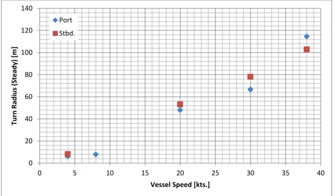
Maneuvering tests were conducted according to the ABS guidelines for vessel maneuverability. Turning circle tests were conducted at 4, 8, 20, & 30 knots and full speed (38 knots). In each case, the steering input was the maximum that the driver deemed possible while maintaining the test speed through the turn (full lock at 4 and 8 knots). Two types of zig-zag tests were conducted: 10 degrees of steering input at 4, 8, 20, & 30 knots and full speed (38 knots), and 20 degrees of steering input at 4 and 8 knots. Both of these tests highlighted the quick handling of the RHIB. In the zig-zag tests a heading change of 10 degrees was achieved in approximately 2 seconds at all speeds (1.5 seconds at full speed) following a 10-degree steering input. In the turning circle tests, the turning radius was less than approximately a boat length at 4 and 8 knots, increasing significantly at higher speeds to 115 m (Port) and 103 m (Stbd.) at 38 knots.
Standing start acceleration tests showed that top speed is achieved in just over 16 seconds over a distance of approximately 250 m. From that speed, the vessel stops in approximately 8.5 s over a distance just greater than 100 m.
Towing tests were conducted with a 65 foot fishing vessel (Roberts Sisters II). A towing speed of 4.6 knots was achieved at full throttle (2,900 rpm). The tow force in this condition was approximately one tonne and fuel consumption was 187 liters per hour, giving a range of just under 10 nm (based on 80% fuel capacity). In the bollard condition, the tow load was just less than one tonne at full throttle (2,600 rpm). In both conditions, it is expected that the achievable tow load would be less than seen in the tests since the vessel was observed to trim by the stern under load. In waves, tow load may have to be limited to prevent swamping.
Seakeeping tests were conducted in three wave states (Hs=.52 m, Tp=2.7 s; Hs=.40 m, Tp=6.5 s; Hs=3.6 m, Tp=11.9s) at different headings. The seakeeping results are very detailed and warrant close examination. Assessments were made of the level of effort required by the driver in each wave state/heading combination and, in general, show that steering input (and deviation from course) increases at low speeds and that the vessel becomes more directionally stable at higher speeds (20 & 30 knots). There is some dynamic instability seen at top speed in long waves. Steeper waves increase the difficulty in maintaining heading and speed as large inputs are required. Steeper waves and higher speeds increase vertical accelerations seen by the vessel hull. Fuel consumption is significantly affected by speed and is relatively insensitive to wave state and heading. The range of the vessel is greatest at low speed but there appears to be a peak in the range between 20 and 30 knots where the vessel can achieve 40 to 50 nautical miles on 80% of its maximum fuel capacity. Further testing is required to define the speed where range is maximized. This work represents a broad baseline of data for fast rescue craft to which alternate designs or equipment can be compared. In order to understand the performance of the diesel engines relative to the conventional gasoline engine configuration, similar testing of the conventional configuration should be conducted.
Table of Contents
Executive Summary ... i
Table of Contents ... ii
Table of Figures ... iv
Table of Tables ... vii
1
Acronyms, Symbols, and Definitions... 1
2
Introduction ... 1
3
Background ... 2
3.1 Vessel Particulars ... 2 3.2 Instrumentation ... 5 3.2.1 CG289 ... 5 3.2.2 Wave Buoys ... 6 3.3 Calibrations ... 64
Tests Completed ... 7
4.1 Maneuvering Tests ... 7 4.1.1 Turning Circles ... 7 4.1.2 Zig-Zags ... 7 4.2 Acceleration Tests ... 74.2.1 Standing Start/Crash Stop ... 7
4.2.2 Acceleration ... 8
4.3 Pull Tests ... 8
4.3.1 Towing Tests ... 8
4.3.2 Bollard Pull Tests ... 9
4.4 Seakeeping Tests ... 9 4.5 Fuel Consumption ... 14
5
Results ... 15
5.1 Maneuvering Tests ... 15 5.1.1 Turning Circles ... 15 5.1.2 Zig-Zags ... 18 5.2 Acceleration Tests ... 235.2.1 Standing Start/Crash Stop ... 23
5.2.2 Acceleration ... 24
5.3 Pull Tests ... 24
5.3.1 Towing Tests ... 25
5.3.2 Bollard Pull Tests ... 26
5.4 Seakeeping Tests ... 27
5.4.1 Degree of difficulty maintaining heading ... 28
5.4.2 Degree of difficulty maintaining speed ... 35
5.4.3 Vessel motions ... 42
5.5 Fuel Consumption ... 1
6
Issues Encountered & Lessons Learned ... 4
7
Recommendations for Future Work ... 4
8
Acknowledgement ... 4
9
References ... 5
Appendix A.
Wave Buoy Specifications ... 1
Appendix B.
Turning Circle Plots ... 2
Appendix C.
Acceleration Plots ... 7
Table of Figures
Figure 2-1. General arrangement of the Zodiac Hurricane 735 SAR configuration [2]. .... 4
Figure 2-2. Sensor locations aboard CG289. ... 6
Figure 3-
1. Plot of CG 289’s track during towing tests. ... 8
Figure 3-2. The setup for the bollard test. The load cell is the yellow part visible adjacent
to the piling. ... 9
Figure 3-3. Detailed view of bollard test towline attachment aboard CG 289. ... 9
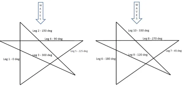
Figure 3-4. Star Patterns, turning to Starboard (on the left) and to Port (on the right). .... 10
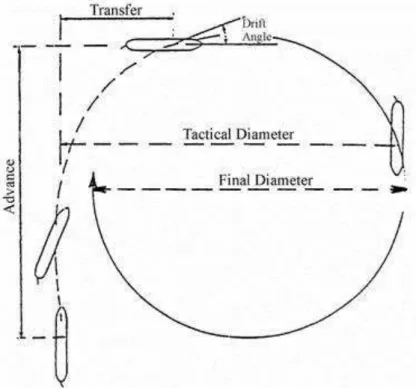
Figure 4-1. Schematic of the values calculated for turning circles. ... 15
Figure 4-2. Turning circle Advance at all speeds tested. ... 16
Figure 4-3. Turning circle Transfer at all speeds tested. ... 17
Figure 4-4. Turning circle Tactical Diameter at all speeds tested. ... 17
Figure 4-5. Turning circle Steady Turn Radius at all speeds tested. ... 18
Figure 4-6. Schematic of the values calculated for zig-zags [3]. ... 19
Figure 4-7. Heading and steering angle plot for the 4 knot 10-10 zig-zag test. ... 20
Figure 4-8. Heading and steering angle plot for the 4 knot 20-20 zig-zag test. ... 20
Figure 4-9. Heading and steering angle plot for the 8 knot 10-10 zig-zag test. ... 21
Figure 4-10. Heading and steering angle plot for the 8 knot 20-20 zig-zag test. ... 21
Figure 4-11. Heading and steering angle plot for the 20 knot 10-10 zig-zag test. ... 22
Figure 4-12. Heading and steering angle plot for the 30 knot 10-10 zig-zag test. ... 22
Figure 4-13. Heading and steering angle plot for the full speed 10-10 zig-zag test. ... 23
Figure 4-14. Speed plotted against time for different initial speeds (0, 4, 8, and 20 knots).
... 24
Figure 4-15. Towing test tow load and vessel pitch as a function of engine rpm (average
P/S). ... 25
Figure 4-16. Bollard test pull load as a function of engine rpm (average P/S). ... 26
Figure 4-17. Bollard test vessel pitch as a function of tow load. ... 27
Figure 4-18. Standard deviation of steering angle for different speeds and headings
relative to wave, WS1. ... 29
Figure 4-19. Standard deviation of steering angle for different speeds and headings
relative to wave, WS2. ... 30
Figure 4-20. Standard deviation of steering angle for different speeds and headings
relative to wave, WS3. ... 31
Figure 4-21. Standard deviation of heading relative to wave (waves from 0 deg) for
different speeds and headings relative to wave, WS1. ... 32
Figure 4-22. Standard deviation of heading relative to wave (waves from 0 deg) for
different speeds and headings relative to wave, WS2. ... 33
Figure 4-23. Standard deviation of heading relative to wave (waves from 0 deg) for
different speeds and headings relative to wave, WS3. ... 34
Figure 4-24. Standard deviation of engine rpm for different speeds and headings relative
to wave, WS1. ... 36
Figure 4-25. Standard deviation of engine rpm for different speeds and headings relative
to wave, WS2. ... 37
Figure 4-26. Standard deviation of engine rpm for different speeds and headings relative
to wave, WS3. ... 38
Figure 4-27. Standard deviation of vessel speed for different speeds and headings relative
to wave, WS1. ... 39
Figure 4-28. Standard deviation of vessel speed for different speeds and headings relative
to wave, WS2. ... 40
Figure 4-29. Standard deviation of vessel speed for different speeds and headings relative
to wave, WS3. ... 41
Figure 4-30. Standard deviation of pitch for different speeds and headings relative to
wave, WS1. ... 43
Figure 4-31. Standard deviation of pitch for different speeds and headings relative to
wave, WS2. ... 44
Figure 4-32. Standard deviation of pitch for different speeds and headings relative to
wave, WS3. ... 45
Figure 4-33. Standard deviation of heave acceleration for different speeds and headings
relative to wave, WS1. ... 46
Figure 4-34. Standard deviation of heave acceleration for different speeds and headings
relative to wave, WS2. ... 47
Figure 4-35. Standard deviation of heave acceleration for different speeds and headings
relative to wave, WS3. ... 48
Figure 4-36. Standard deviation of roll for different speeds and headings relative to wave,
WS1. ... 49
Figure 4-37. Standard deviation of roll for different speeds and headings relative to wave,
WS2. ... 50
Figure 4-38. Standard deviation of roll for different speeds and headings relative to wave,
WS3. ... 51
Figure 4-39. Fuel Consumption as a function of vessel Speed, for all star pattern tests. ... 2
Figure 4-40. Fuel consumption as a function of engine speed for free-running (star tests,
towing, and bollard conditions. ... 2
Figure 4-41. . Fuel consumption as a function of engine speed for free-running (star tests,
towing, and bollard conditions (zoomed-in). ... 3
Figure 4-42. Predicted vessel range as a function of speed for free-running and towing
conditions (using 80% fuel capacity = 400 litres). ... 3
Figure B-1. Port and Starboard turning circle tracks at 4 knots. ... 2
Figure B-2. Port and Starboard turning circle tracks at 8 knots. ... 3
Figure B-3. Port and Starboard turning circle tracks at 20 knots. ... 4
Figure B-4. Port and Starboard turning circle tracks at 30 knots. ... 5
Figure B-5. Port and Starboard turning circle tracks at full speed (~38 knots). ... 6
Figure C-1. Speed, rpm, and distance plotted against time (Standing Start/Crash Stop #1).
... 7
Figure C-2. Speed, rpm, and distance plotted against time (Standing Start/Crash Stop #2).
... 8
Figure C-3. Speed, rpm, and distance plotted against time (Standing Start/Crash Stop #3).
... 9
Figure C-4. Speed, rpm, and distance plotted against time (Standing Start/Crash Stop #4).
... 10
Table of Tables
Table 3-1. Principal particulars of CG 289. ... 2
Table 3-
2. Calculation of “as-tested” loading condition ... 3
Table 3-3. Sensors aboard CG289. ... 5
Table 4-1. Summary of target Turning Circle test parameters. ... 7
Table 4-2. Star patterns executed in Wave State 1 (Nov. 14, 2016) and wave statistics. . 11
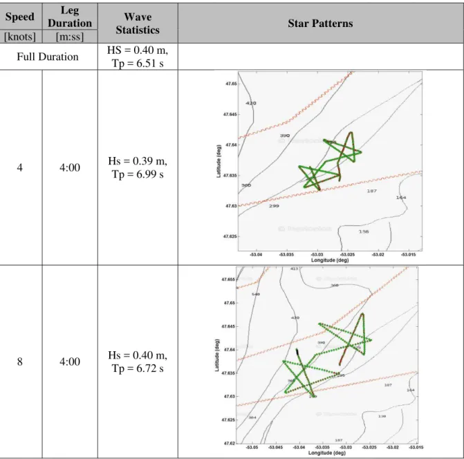
Table 4-3. Star patterns executed in Wave State 2 (Nov. 17, 2016) and wave statistics. . 12
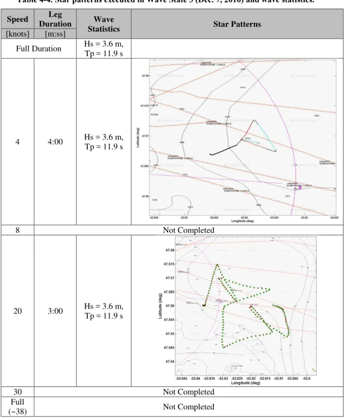
Table 4-4. Star patterns executed in Wave State 3 (Dec. 7, 2016) and wave statistics. ... 14
Table 5-1. Summary of turning circle test results. ... 16
Table 5-2. Summary of target zig-zag test parameters. ... 19
Table 5-3. Zig-zag test results. ... 19
Table 5-4. Summary of Acceleration/Deceleration times and distances (Standing
Start/Crash Stop tests). ... Error! Bookmark not defined.
Table 5-5. Summary of towing test conditions & results. ... 25
1
1
Acronyms, Symbols, and Definitions
B “Beam”
FRC “Fast Rescue Craft”
LCG “Longitudinal Center of Gravity” LOA “Length Overall”
RHIB “Rigid Hull Inflatable Boat” SAR “Search and Rescue” VCG “Vertical Center of Gravity”
“Displacement”
Kiting When a vessel loses control due to becoming airborne at the crest of a wave. Pitch poling When a vessel’s bow is buried in the back of a wave while surfing. This can
cause the vessel to become submerged and, in extreme cases, flipping end-over-end.
2
Introduction
Testing was carried out on board CG 289, a Canadian Coast Guard Search and Rescue Fast Response Craft during November and December 2016 in Conception Bay and outside St. John’s harbor, Newfoundland & Labrador. These tests were a part of the evaluation of a new engine configuration.
The vessel tested is a Zodiac Hurricane 753 RHIB in SAR configuration, equipped with twin Mercury Marine DSI 3.0 diesel outboard motors. The tests were conducted with the typical crew compliment of three and each test day began with a full fuel load.
The goals of this test were threefold:
1. To Gain experience with packaging instrumentation aboard a small, fast vessel, and demonstrate the value in the data that can be collected.
2. To quantify the performance of the engines.
3. To assess the performance of the RHIB in real-world conditions. These goals were fulfilled through a series of tests, comprised of:
1. Maneuvering tests (steady-state turning and zig-zags)
2. Acceleration tests (acceleration under full power and deceleration under zero power) 3. Pull tests (bollard and towing)
4. Seakeeping tests (star patterns in varying wave state) 5. Fuel consumption (collected during star pattern tests) 6. Normal vessel operation (not included in report)
These tests provide a data set that can be used to understand the performance and operation of the vessel and, perhaps more importantly, form the baseline for future procurement specifications and/or assessment of different platforms.
3 Background
Test locations were selected based on being near enough to St. John’s to prevent extended travel, and likely to provide testing conditions representative of SAR operations. Testing was conducted based out of the inshore SAR base at the Royal Newfoundland Yacht Club in Manuels, NL and out of the Canadian Coast Guard base in St. John’s, NL.
3.1 Vessel Particulars
The principal particulars of CG 289 are listed in Table 3-1, the as-tested load condition, including assumed mass and location of load items is summarized in
Table 3-2, and the general arrangement of the vessel is provided in Figure 3-1.
All tests discussed in this report were completed with 4-17 (four-bladed, 17 inch pitch) propellers. No modifications were made to the vessel other than to mount sensors and data acquisition hardware and these were designed to be as unobtrusive as possible. All equipment was installed so that no permanent changes were made to the vessel; everything could be put back to the original state following testing. The instrumentation installed is discussed on page 5.
All test days began with full fuel tanks in order to ensure a consistent mass and mass distribution from day to day. With small vessels, the crew makes up a significant portion of the total mass and has a significant effect on the center of gravity. During operation, particularly in waves, the crew moved around the boat somewhat to shield themselves from water spray. While this movement is not ideal from the perspective of scientific control, it is expected to be indicative of real-world operation and, consequently, consistent with the goals of this work.
Table 3-1. Principal particulars of CG 289.
LOA 8.15 m BMAX 2.75 m LS 2,100 kg LCGLS (fwd of keel/transom) 2.118 m VCGLS (above keel/transom) 0.388 m MAX 3,823 kg LCGMAX (fwd of keel/transom) 2.273 m
VCGMAX (above keel/transom) 0.714
Fuel Capacity (fuel tanks were filled prior to each test day)
321 l (main) + 181 l (reserve) approx. 241 kg + 136 kg Source: [1, 2]
3 Table 3-2. Calculation of “as-tested” loading condition
Item Mass LGC VCG LCG Moment VCG Moment [kg] [m fwd of keel/transom] [m above keel/transom] [kg∙m] [kg∙m] Light Ship 2,100 2.118 0.388 4447.8 814.8 Driver 120 2.298 1.342 275.8 161.0 Crew 2 120 1.320 1.342 158.4 161.0 Crew 3 120 1.320 1.342 158.4 161.0 Fuel 1 241 4.675 0.397 1126.7 95.7 Fuel 2 136 3.043 0.452 413.8 61.5 Sum 2,837 6580.9 1455.1 As Tested 2,837 2.320 0.513
5
3.2 Instrumentation
Data was collected from three sources throughout the testing: Data acquisition system aboard CG289
Large wave buoy (moored) Small wave buoy (drifting)
3.2.1 CG289
The primary instrumentation used for the testing was installed aboard CG289. A bespoke data acquisition system was installed inside the forward console (below the steering wheel) which included a six degree-of-freedom inertial sensor and connected to additional sensors installed throughout the vessel as well as the engines’ stock telemetry system. The list of data being acquired aboard CG289 is shown in Table 3-3.
Table 3-3. Sensors aboard CG289.
Data Source (Locations shown in Figure 3-2)
Vessel Motions
Roll, Pitch, & Yaw rate
Heave, Surge, & Sway acceleration1
6 DoF inertial sensor Vessel Speed
GPS, DGPS Vessel Heading
Latitude, Longitude
Wind Speed & Direction Doppler Anemometer Forward (crew), Aft (engines) video Video Cameras Air Temperature2
Mercury “SmartCraft” system Engine RPM (P & S)
Battery Voltage2
Alternator Voltage (P & S)2 Engine Tilt (P&S)2
Fuel Consumption (P & S) Coolant Pressure (P&S)2
1. Heave, surge, & sway acceleration values reported at the sensor, approx. 2.82 m forward of and 0.88 m above keel/transom (in the forward console, see Figure 3-2).
Figure 3-2. Sensor locations aboard CG289.
Heave, surge, & sway values reported at the sensor, approx. 2.82 m forward of and 0.88 m above keel/transom (in the forward console).
3.2.2 Wave Buoys
Two wave buoys were used to measure the wave state during testing. For testing in Conception Bay (Nov. 14, 2016, Nov. 17, 2016), A TRYAXISTM Directional Wave Buoy was used, moored at 47.53⁰N, 53.08⁰W. This wave buoy was deployed Nov. 7, 2016 and remained in place throughout the testing. The location for mooring the wave buoy was selected in an area of relatively constant depth and away from the islands in Conception Bay to minimize changes in the wave state through the test area due to depth variation or island proximity.
During the day of testing off St. John’s harbor (Dec. 7, 2016), a TRYAXISTM
Mini Wave Buoy was used. The wave buoy was deployed from a second CCG RHIB upwind of the intended test area, was allowed to drift throughout the test, and was retrieved immediately following the test. The specification sheets for the two wave buoys are attached in Appendix A.
3.3 Calibrations
The instrumentation employed in this system was almost exclusively digital in nature and in such will be both functional and accurate (within its’ respective specifications) or completely non-functional. The exception to this is the analog displacement sensor (an ILPS-19-200-00-R-10-A, Linear Inductive Sensor) used to measure steering angle.
The steering angle sensor was mounted in tandem with the starboard steering actuator and by observing the extension / retraction of this actuator a proportional measure of steering angle was obtained. Output from this device was in volts and a proportionality / absolute value transfer function (y=mx+b) was derived by recording steering angle physically and electronically throughout the measurement range. With the boat on the trailer and the transom perpendicular to the floor a quadrant type target was placed below the starboard outboard. Using a plumb bob the position of the starboard outboard was transferred to the target at various steering angles over the range of articulation. Angles noted on the target quadrant were measured graphically and, when compared to recorded signals from the sensor, a calibration factor and absolute angle measurement were derived.
Doppler Anemometer
Acquisition System & Inertial Sensor (Inside Console)
GPS, DGPS Cameras
7
4 Tests Completed
4.1 Maneuvering Tests
Two types of maneuvering tests were completed: Turning Circles and Zig-Zags. These tests are based on the guidelines provided by the American Bureau of Shipping [3].
4.1.1 Turning Circles
The instructions provided to the helmsman during the turning circle tests were to achieve the steady-state speed desired for the test before turning to port. Following two complete circles to port, the wheel was moved to midships and then the same amount to starboard for two complete circles. Throughout both turns, the throttle was varied to maintain a constant speed. The amount that the wheel was turned for these tests was selected as being the tightest turn in which the desired speed could be maintained based on the helmsman’s experience. The target parameters for these tests are summarized in
Table 4-1. Summary of target Turning Circle test parameters. Speed over
Ground
Steering Input
[knots] [turns] [degrees]
4 Full Lock 22 (S), 26 (P) 8 Full Lock 22 (S), 26 (P) 20 1 10 30 1 10 Full (~38) ¾ 7.5 4.1.2 Zig-Zags
Two types of Zig-Zag tests were performed: “10-10 zags” and “20-20 zags”. In 10-10 zig-zags, the helm is nominally altered ten degrees until the vessel’s heading answers ten degrees at which point the helm is altered ten degrees the other way until the vessel’s heading answers ten degrees. This procedure is repeated through three to four cycles. For 20-20 zig-zags, the procedure is the same except that the help input and heading response are both twenty degrees. For purposes of practicality aboard the RHIB (since no helm input readout was available) the helm inputs were selected as one full turn (10-10 zig-zag) and two full turns (20-20 zig-zag).
4.2 Acceleration Tests
Acceleration tests were performed from a standing start as well as from steady-state speeds of 4, 8, & 20 kts. All of these tests were performed in calm water with low wind. In order to cancel out any effects of wind, tests were performed in an out-and-back fashion (eg, upwind and downwind).
4.2.1 Standing Start/Crash Stop
Standing Start/Crash Stop tests were performed to assess the longitudinal acceleration and deceleration of the vessel. From zero forward speed (<0.5 knots), the throttles were advanced rapidly to full throttle and held in this position until maximum speed was reached (~38 knots). At this point, the throttles were pulled back to neutral and the vessel was allowed to slow down naturally. The throttles were not put into reverse during this maneuver due to concerns that this would damage the gear boxes and/or propellers.
4.2.2 Acceleration
This set of tests was intended to investigate the difference (if any) between accelerating from stopped and accelerating from a constant initial speed. For these tests, helmsmen were instructed to hold the steady-state start speed for a period before rapidly advancing the throttles to full throttle and maintaining full throttle until full speed (or near full speed) had been achieved.
4.3 Pull Tests
Two types of pull tests were performed: bollard pulls (zero forward speed) and towing a vessel typical of the type that may be towed during rescue operations.
4.3.1 Towing Tests
Towing tests were performed in relatively flat water in St. John’s harbor with the FV Roberts Sisters II as the vessel being towed. While the water was calm, there was a wind of 15-20 knots from the SW.
During the towing tests, throttle was increased in steps to achieve a target rpm while maintaining a consistent pull angle as much as possible. Approximately 50 m of CG289’s towing line was paid out and connected to the bow of the Roberts Sisters II. The towing load cell was connected in-line with the tow line.
A summary of the track followed during the towing test is presented in Figure 4-1. Only data from the upwind portion of the testing (moving from upper right to lower left) is reported. Data “dropouts” were experienced during this test and are discussed more fully in Section 6, Issues Encountered.
9
4.3.2 Bollard Pull Tests
A set of bollard pull (zero forward speed) tests was performed from idle engine speed up through the engines’ operating range to full throttle, in steps of approximately 500 rpm. In the bollard condition, the engines achieved approximately 2,600 rpm. From full throttle, the engines were slowed down to idle in steps of approximately 1,000 rpm.
Pull load was measured by an inline load cell. CG 289’s tow line was used, connected to the tow post of CG 289 at one end and the load cell at the other end. The load cell, in turn, was attached to a piling with a webbing strap. During the test, the tow line and load cell were approximately horizontal. During the test, the tow line was tied off with approximately 50 m paid out. The set up for the bollard test is shown in Figure 4-2 (with the line not fully paid out) and a detailed view of the connection to CG 289 is shown in Figure 4-3.
Figure 4-2. The setup for the bollard test. The load cell is the yellow part visible adjacent to the piling.
Figure 4-3. Detailed view of bollard test towline attachment aboard CG 289.
4.4 Seakeeping Tests
Star pattern tests were conducted to assess seakeeping in different wave states. These tests involved steering ten prescribe courses relative to the wave direction as shown in Figure 4-4. Star tests were performed at the speeds shown in Table 4-2, Table 4-3, & Table 4-4 and summarized below:
In wave state 1 (Table 4-2), tests at 30 kts and full speed were not attempted due to concerns that the boat would “kite” over the short, steep waves. Even at 20 kts, certain headings resulted in noticeable propeller ventilation.
In wave state 2 (Table 4-3), tests were completed at all target speeds (4 kts, 8 kts, 20 kts, 30 kts, & full speed).
In wave state 3 (Table 4-4), a partial test was completed at 4 kts and a test was completed at 20 kts before deciding to abandon the remainder of the tests due to safety concerns related to operating in the worsening weather (high wind and wave state).
Each heading was maintained for the time shown in Table 4-2, Table 4-3, & Table 4-4. As speed increased, the time duration at each heading was reduced to restrict operation to a reasonable area. Some difficulty was found on maintaining the desired heading due to the delayed response of both the magnetic compass and the GPS heading. This was particularly prevalent at low speeds and/or in high waves. Table 4-2, Table 4-3, & Table 4-4 show the achieved track for each set of tests. The data was analyzed to account for these discrepancies between the desired and achieved heading and all data is reported with the achieved heading.
11 Table 4-2. Star patterns executed in Wave State 1 (Nov. 14, 2016) and wave statistics. Speed Leg
Duration Wave
Statistics Star Patterns
[knots] [m:ss] Full Duration Hs = 0.52 m, Tp = 2.71 s 4 4:00 Hs = 0.43 m, Tp = 2.51 s 8 4:00 Hs = 0.55 m, Tp = 2.76 s 20 3:00 Hs = 0.59 m, Tp = 2.87 s 30 Not Completed Full (~38) Not Completed
Table 4-3. Star patterns executed in Wave State 2 (Nov. 17, 2016) and wave statistics. Speed Leg
Duration Wave
Statistics Star Patterns
[knots] [m:ss] Full Duration HS = 0.40 m, Tp = 6.51 s 4 4:00 Hs = 0.39 m, Tp = 6.99 s 8 4:00 Hs = 0.40 m, Tp = 6.72 s
13 20 3:00 Hs = 0.40 m, Tp = 6.60 s 30 2:00 Hs = 0.41 m, Tp = 6.32 s Full (~38) 1:30 Hs = 0.40 m, Tp = 5.93 s
Table 4-4. Star patterns executed in Wave State 3 (Dec. 7, 2016) and wave statistics. Speed Leg
Duration Wave
Statistics Star Patterns
[knots] [m:ss] Full Duration Hs = 3.6 m, Tp = 11.9 s 4 4:00 Hs = 3.6 m, Tp = 11.9 s 8 Not Completed 20 3:00 Hs = 3.6 m, Tp = 11.9 s 30 Not Completed Full (~38) Not Completed 4.5 Fuel Consumption
No specific tests were completed to assess fuel consumption. Rather, fuel consumption was assessed throughout the trials for a range of operational parameters. During testing, several high speed runs were made with speeds near maximum speed in nearly calm water sustained for extended periods of time (> 10 minutes). These runs allow specific assessment of fuel consumption at high speed. In addition, fuel consumption was calculated on each leg of the
15 seakeeping tests, allowing comparison of fuel consumption in different speeds, wave states, and wave directions. The limited duration of these tests, however, resulted in limited data which should only be used for high level comparison rather than any sort of prediction of fuel consumption.
5 Results
5.1 Maneuvering Tests 5.1.1 Turning Circles
The key results for the turning circle tests (see Figure 5-1) are presented in Table 5-1. How each parameter varies with increasing speed is also presented graphically (Advance: Figure 5-2, Transfer: Figure 5-3, Tactical Diameter: Figure 5-4, and Steady Turn Radius: Figure 5-5).
Some asymmetry is observed in these results (ie, results turning to port are not the same as results turning to starboard). The source of this is unknown. In general, the port-turning circle was completed before the starboard turning circle, meaning that there was a shorter period of steady-state prior to the starboard turning circle. This is not believed to be the source of the asymmetry, however, since the asymmetrical turning performance was noticed elsewhere during the testing with the vessel consistently turning more tightly to port.
Table 5-1. Summary of turning circle test results. Speed
P/S Advance Transfer Tactical Diameter Turn Radius
[knots] [m] 4 Port 19.1 3.2 20.6 6.2 8 19.5 1.4 23.1 7.9 20 49.2 16 85 48 30 93.7 20.6 124.8 66.6 38 180.3 72.4 240.1 114.6 4 Stbd. 15.3 5.7 15.1 8.1 20 66.6 52.7 102.6 53.2 30 80.2 81.9 148.7 78.1 38 112.4 108.8 177.3 102.9
Figure 5-2. Turning circle Advance at all speeds tested.
0 20 40 60 80 100 120 140 160 180 200 0 5 10 15 20 25 30 35 40 A d v an ce [ m ] Vessel Speed [kts.] Port Stbd.
17 Figure 5-3. Turning circle Transfer at all speeds tested.
Figure 5-4. Turning circle Tactical Diameter at all speeds tested.
0 20 40 60 80 100 120 0 5 10 15 20 25 30 35 40 Tr an sf e r [ m ] Vessel Speed [kts.] Port Stbd. 0 50 100 150 200 250 300 0 5 10 15 20 25 30 35 40 Tact ic al D iam e te r [ m ] Vessel Speed [kts.] Port Stbd.
Figure 5-5. Turning circle Steady Turn Radius at all speeds tested.
5.1.2 Zig-Zags
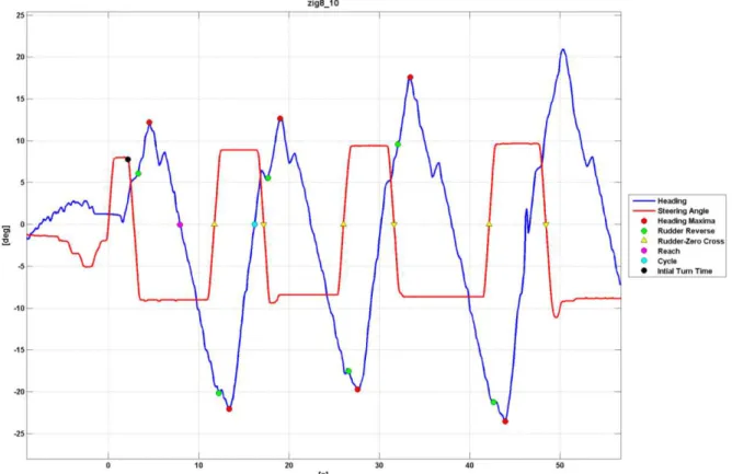
The quick response of the boat to steering inputs made it difficult to read the compass or the GPS heading readout while simultaneously steering the boat. As it was, significant difficulty was encountered in reliably determining when the desired heading had been achieved due to lag in the instruments. Helmsmen resorted to using distant landmarks to determine when the desired heading had been reached. The 20-20 zig-zags could not be attempted at speeds above 8 knots. Table 5-2 summarizes the target test parameters for the zig-zag tests. There is some discrepancy between the target heading and the achieved heading which highlights the difficulty of precisely judging heading while steering a vessel that responds so quickly. The vessel does respond very quickly to steering inputs; the initial turn time for the 10 degree tests (ie, the time to reach 10 degrees after steering input is initiated) varies between 1.5 and 2.3 seconds. Interestingly, judging by the reach and cycle times, the vessel responds slowest at 8 knots (taking longer to complete a cycle).
The results of the zig-zag tests are shown in Table 5-3. The values reported are those recommended by the American Bureau of Shipping for maneuvering tests [3]. Plots of the steering input and heading response are shown in Figure 5-7 to Figure 5-13. These plots show that, while there was some variation in heading maxima and in steering input, the input and response were quite consistent within a given test as a result of the strategies of gauging input by the number of steering wheel turns and heading by using a landmark. Examining the time scale of these plots also highlights the quick response of the vessel; during tests at top speed, a constant steering input was held for approximately a second before the heading responded to 10 degrees.
0 20 40 60 80 100 120 140 0 5 10 15 20 25 30 35 40 Tu rn R ad iu s (Ste ad y ) [m ] Vessel Speed [kts.] Port Stbd.
19 Table 5-2. Summary of target zig-zag test parameters.
Zig-zag type
Speed Steering Input [knots] [turns] [degrees]
(approx.) 10-10 4 1 10 8 1 10 20 1 10 30 1 10 Full (~38) 1 10 20-20 4 2 20 8 2 20
Figure 5-6. Schematic of the values calculated for zig-zags [3]. Table 5-3. Zig-zag test results.
Zig-zag type 10-10 20-20
Speed [kts] 4 knot 8 knot 20 knot 30 knot 38 knot 4 knot 8 knot Initial turn time [s] 2.22 2.17 2.20 1.42 2.07 5.42 3.09 Reverse rudder heading
angle [deg] 2.54 6.10 8.87 11.6 12.6 31.5 42.3
1st overshoot angle [deg] -5.94 2.21 -0.838 3.52 6.89 12.3 23.3 2nd overshoot angle [deg] -1.01 12.1 0.845 -0.894 -5.41 19.5 3.45 Time to check yaw [s] 2.00 2.36 1.18 0.910 0.620 3.40 2.11 Reach (1st cycle) [s] 5.54 7.93 4.79 4.05 5.12 11.8 10.9 Cycle Time [s] 10.8 16.2 8.21 7.05 7.01 22.6 17.5
Figure 5-7. Heading and steering angle plot for the 4 knot 10-10 zig-zag test.
21 Figure 5-9. Heading and steering angle plot for the 8 knot 10-10 zig-zag test.
Figure 5-11. Heading and steering angle plot for the 20 knot 10-10 zig-zag test.
23 Figure 5-13. Heading and steering angle plot for the full speed 10-10 zig-zag test.
5.2 Acceleration Tests
5.2.1 Standing Start/Crash Stop
Four tests were completed to assess acceleration from a standing start and a crash stop (zero throttle). The results are summarized in stern wave catches the vessel.
. Plots of speed and engine rpm against time are shown in Figure C-1 to Figure C-4.
There was some difficulty in determining the time that the vessel reached maximum speed and the time that the vessel “stopped” since the accelerations were quite low at these time (ie, the speed curve was quite flat).
To assist with determining the time that the vessel stopped (since the vessel never truly stops), a threshold of 4 knots was selected as “stopped”. During deceleration, the vessel slows rapidly at first and then deceleration decreases as the vessel slows. Near four knots, there is a small acceleration due to the vessel ceasing to plane and being caught by the stern wave which pushes the vessel slightly, causing a temporary acceleration. While Figure C-3 and Figure C-4 show the “stopped’ criterion occurring after this effect, the data reported in Table 5-4 is based on the minimum speed occurring before the stern wave catches the vessel.
Table 5-4. Summary of Acceleration/Deceleration times and distances (Standing Start/Crash Stop tests).
Time to Max. Speed
Time to Stop Distance to Max. Speed Distance to Stop [s] [m] Mean 16.26 8.60 245.2 103.5 Std. Dev. 1.77 0.45 24.80 17.26 Range (± 1 Std. Dev.) 14.48 - 18.02 8.14 - 9.04 220.4 - 270.0 86.19 - 120.7 5.2.2 Acceleration
A plot of speed against time is shown in Figure 5-14, comparing the acceleration from a steady speed of 20, 8, and 4 knots to the acceleration curve from zero speed. This data shows that, upon application of full throttle, the vessel follows nearly the same acceleration curve from all initial speeds. Initial speed has very little effect on the acceleration rate. This may be expected to change if different propellers were used as more aggressive propellers would reduce the engines’ ability to spin up, thereby resulting in a more gradual approach to the steady acceleration curve.
Figure 5-14. Speed plotted against time for different initial speeds (0, 4, 8, and 20 knots).
5.3 Pull Tests
Two types of pull tests were conducted: Towing (variable forward speed) and Bollard (zero forward speed).
The Towing tests were conducted at a range of speeds from 0.5 to 4.6 knots, resulting from approximately 1000 rpm to 3,000 rpm engine speed. This test was stopped due to the engines beginning to ‘surge’ under load but 3,000 rpm also represents nearly full throttle.
The bollard tests were completed from idle speed (~625 rpm) to 2,625 rpm. 2,625 rpm represents full throttle in the bollard condition.
25 Overall, more tow load was generated during the forward speed towing test than in the bollard condition. This is expected to be due to the higher engine rpm attained. This assumption could be tested by examination of the propeller torque curves and engine torque characteristics. The towing tests also result in more bow-up vessel pitch due to the combination of towing and hydrodynamic loads. While transom submersion was not a great concern during bollard tests, there was concern of transom submersion during the towing tests. This concern would limit the towing capabilities in even a slight seaway as engine rpm would have to be reduced to avoid swamping.
5.3.1 Towing Tests
The results of the towing tests are shown in Table 3-1 and a plot of the tow load and tow speed against engine rpm are shown in Figure 5-15. Both tow load and tow speed increase in a linear fashion with increasing engine rpm. The maximum tow load achieved was 10,000 N at a speed of 4.6 knots (2,900 rpm).
Table 5-5. Summary of towing test conditions & results.
Engine Speed Achieved Speed Tow Load1 Vessel Pitch Total Fuel Consumption [rpm, average P, S] [knots] [N] [deg, + bow up] [litres per hour]
965 0.52 1,373
1,204 1.45 2,599 6.2 25.9
2,089 1.94 6,866 7.3 90.6
2,572 3.49 9,318 7.8 139.9
2,913 4.60 10,102 8.1 187.3
1. Tow load data recorded manually, not integrated into data acquisition system. 2. Data not available from data acquisition system. Speed recorded manually from GPS
readout, engine rpm recorded manually from observation.
Figure 5-15. Towing test tow load and vessel pitch as a function of engine rpm (average P/S). 0 0.5 1 1.5 2 2.5 3 3.5 4 4.5 5 0 2,000 4,000 6,000 8,000 10,000 12,000 0 500 1,000 1,500 2,000 2,500 3,000 3,500 To w S p e e d [kt s] To w Load [ N ] Engine rpm
Tow Load Tow Speed
5.3.2 Bollard Pull Tests
The results of the bollard pull test are shown in Table 5-6. The maximum achieved pull load in the bollard condition was 9,800 N at 2,625 rpm. Figure 5-16 shows a plot of the achieved pull load as a function of rpm and Figure 5-17 shows the vessel pitch (positive bow-up) as a function of tow load.
Table 5-6. Summary of bollard test conditions and results. Engine Speed Tow Load1 Vessel Pitch [rpm, average P, S] [N] [deg, + bow up]
625 510 3.9 958 1,324 3.4 1,164 1,079 3.8 1,516 3,237 4.1 2,005 5,885 5.0 2,036 6,179 5.3 2,478 8,925 5.9 2,625 9,808 6.1
1. Tow load data recorded manually, not integrated into data acquisition system.
Figure 5-16. Bollard test pull load as a function of engine rpm (average P/S).
0 2,000 4,000 6,000 8,000 10,000 12,000 0 500 1,000 1,500 2,000 2,500 3,000 Pu ll Load [N ] Engine rpm
27 Figure 5-17. Bollard test vessel pitch as a function of tow load.
5.4 Seakeeping Tests
The results of seakeeping tests are presented in this section as polar plots with the results for each heading plotted around a circle and the distance from the center of the plot to the point indicating the magnitude. In each case, the reported course is relative to the wave direction (ie, 0 degrees indicates head seas and 180 degrees indicates following seas). The achieved heading angles relative to the wave direction differ from the target heading angles primarily due to uncertainty in determining the wave direction.
For each parameter, the data for all speeds is presented on one plot with separate plots for each sea state. The parameters presented are:
Difficulty maintaining heading
o Standard deviation of steering angle o Standard deviation of heading Difficulty maintaining speed
o Standard deviation of engine rpm (as a proxy for throttle input) o Standard deviation of vessel speed
Vessel motions
o Standard deviation of pitch o Standard deviation of heave o Standard deviation of roll
Overall, the degree of difficulty in maintaining heading was highest in steep waves and at low speeds. At top speed, there was also some directional instability observed, particularly in beam and quartering waves. The results for degree of difficulty in maintain speed were similar in that steep waves required more throttle input variation and saw more significant changes in speed. Maintaining speed was most difficult in head and following seas and least difficult in beam seas.
0 1 2 3 4 5 6 7 0 2,000 4,000 6,000 8,000 10,000 12,000 Pi tc h [ d e g ] Tow Load
Heave acceleration increased with speed in all wave states with a several observations recording in excess of 4.5 times the acceleration due to gravity in WS2. In the small, steep waves of WS1, the hull shape was most efficient at absorbing wave impacts.
5.4.1 Degree of difficulty maintaining heading
The degree of difficulty associated with maintaining a consistent course in each wave condition and heading was assessed by looking at the standard deviation of two factors:
1. The steering angle, indicating how much the driver has to alter the steering input to maintain speed.
2. The vessel heading, indicating to what degree the driver is successful at maintaining heading.
From the diagrams presented in Figure 5-18 to Figure 5-20, it can be seen that the effort of the driver (as shown by the standard deviation in steering input) is highest in steeper waves (WS1 and WS3, Figure 5-18 & Figure 5-20). This is most pronounced in bow and stern quartering waves as the vessel is heavily influenced by the wave while climbing and descending the face and back of the wave. In longer, less-steep waves (WS2, Figure 5-19), the steering input is less than in steeper waves. The degree of success at following the average course closely mirrors the effort being put in by the driver; in most cases, the driver input seems to be driven by large deviations in heading (Figure 5-21 to Figure 5-23).
In all wave types tested, there is more steering input required to maintain course at low speeds than at higher speeds up to 20 knots, indicating that the vessel becomes more directionally stable at higher speeds. There is a limit to the directional stability, however, as seen at full speed (~38 knots) in WS2 where a significantly higher steering input was required to maintain course, particularly in bow quartering waves. In these cases, not only is the steering input higher but so is the deviation from course (Figure 5-22), indicating that (despite the effort) the driver is not able to maintain a steady course with standard deviation of heading between nearly 20 to nearly 30 degrees, depending on the wave encounter angle. At 30 knots, this increased deviation in heading is also seen, albeit to a lesser extent than at top speed.
29 Figure 5-18. Standard deviation of steering angle for different speeds and headings relative to wave, WS1.
31 Figure 5-20. Standard deviation of steering angle for different speeds and headings relative to wave, WS3.
33 Figure 5-22. Standard deviation of heading relative to wave (waves from 0 deg) for different speeds and headings relative to wave, WS2.
35
5.4.2 Degree of difficulty maintaining speed
The degree of difficulty associated with maintaining speed in each wave condition and heading was assessed by looking at the standard deviation of two factors:
1. Standard deviation of engine rpm (as a proxy for throttle position), indicating how much the driver has to alter the throttle setting to maintain speed. Rpm is also related to engine loading so variations in rpm indicate variations in throttle and/or loading, both indicating difficulty in maintaining speed.
2. Standard deviation of vessel speed, indicating to what degree the driver is successful at maintaining speed.
In WS1 and WS3, where 20 knots was deemed to be the maximum safe speed, the driver identified that throttle had to be varied to prevent ‘kiting’ over the crest of waves and ‘pitch poling’ in the troughs. For this reason, relatively high standard deviations are observed of up to 250 rpm for WS1 (Figure 5-24) and 450 rpm for WS3 (Figure 5-26). In the short, steep waves of WS1, high variations in throttle input were also seen, due to the tendency for the vessel to slow down when climbing waves and surf when descending.
WS2 (Figure 5-25) provided the clearest pattern of throttle variation needed to maintain speed. With standard deviations of about 125 rpm to 175 rpm in head seas with comparatively small engine rpm standard deviations in beam seas (25 rpm to 75 rpm) and following seas (50 rpm to 150 rpm). At full speed, high variations in throttle input were also seen in beam seas (125 rpm to 175 rpm).
In general, greater variations in vessel speed (Figure 5-27 to Figure 5-29) correspond to greater driver effort to maintain speed. This is particularly prevalent in the tests at 20 knots in WS1 and WS3 where the driver was working particularly hard to prevent ‘kiting’ and ‘pitch poling’.
37 Figure 5-25. Standard deviation of engine rpm for different speeds and headings relative to wave, WS2.
39 Figure 5-27. Standard deviation of vessel speed for different speeds and headings relative to wave, WS1.
41 Figure 5-29. Standard deviation of vessel speed for different speeds and headings relative to wave, WS3.
5.4.3 Vessel motions
Interestingly, the standard deviation of pitch is relatively consistent for all speeds in a given wave state with a significant increase only near the limit of operation (20 knots in WS1 and WS3 and 38 knots in WS2). At lower speeds, there is generally more pitch in head seas, followed by following seas, and the least pitch is observed in beam seas. At the limit of operation, pitch increases significantly in beam seas.
Heave acceleration (“Acceleration_Z”) data is reported for the sensor location which is inside the forward (driver’s) console, about 200 mm above the floor of the RHIB. It is possible to translate this motion to points of interest but this is beyond the scope of this project as no points of interest were identified. The heave as reported corresponds roughly to the heave felt by the driver.
Significant heave accelerations are felt at speeds near the limits of operation with a steady increase in heave acceleration variation seen with increasing speed. The maximum heave acceleration felt was in the range of 4.5 times gravity, at a number of headings at full speed in WS2. This observation, combined with the observation that variations in heave acceleration are quite low for low speeds in all waves tested, indicate that at low speeds, the vessel’s hull effectively absorbs energy from the waves, reducing acceleration. The hull is particularly effective at absorbing impacts from head seas in short, steep waves such as WS1.
It is important to note that the vertical accelerations felt by the crew are less than those felt by the hull due to the shock-absorbing seats and the crew using their legs to absorb impacts. Accelerations at the shock absorbing seats or of the crew’s bodies were not measured.
43 Figure 5-30. Standard deviation of pitch for different speeds and headings relative to wave, WS1.
45 Figure 5-32. Standard deviation of pitch for different speeds and headings relative to wave, WS3.
47 Figure 5-34. Standard deviation of heave acceleration for different speeds and headings relative to wave, WS2.
49 Figure 5-36. Standard deviation of roll for different speeds and headings relative to wave, WS1.
51 Figure 5-38. Standard deviation of roll for different speeds and headings relative to wave, WS3.
1
5.5 Fuel Consumption
Based on the fuel consumption data for the star pattern tests, there is very little correlation between fuel consumption and heading relative to wave with an overall correlation coefficient of 0.0570. Individual correlations between fuel consumption and heading relative to wave vary between 0.2600 (WS3) and -0.0031 (WS2). This means that the heading relative to the wave affects the fuel consumption more in severe waves. There is little correlation, however, between the wave state and the fuel consumption: Correlation between Hs and fuel consumption is
-0.02552 and correlation between Tp and fuel consumption is 0.1116.
There is strong correlation between fuel consumption and speed with an overall correlation of 0.9893 based on data for all wave states. This correlation is strongest in Wave State 2 (0.9862) and weaker in WS1 (0.9758) and WS3 (0.9434). Figure 5-39 shows the fuel consumption data plotted against vessel speed for all of the star tests (all headings and wave states). From this data, it can be calculated that, from 4 to 30 knots, a one-knot increase in speed requires approximately 9 liters per hour in additional fuel. Between 30 knots and 38 knots, this marginal consumption rate increases drastically to about 18 liters per hour in additional fuel required to increase speed by one knot.
Fuel consumption is also influenced by the load experienced by the engines. Figure 5-40 compares the fuel consumption as a function of engine speed for three conditions: free-running (star pattern tests), towing, and bollard. Figure 5-41 shows the same data over the rpm range seen in the towing and bollard tests. A significant increase in fuel consumption is seen at comparable engine speeds between the free-running condition and the towing condition (about a 36 % increase at 2,600 rpm) and again from the towing condition to the bollard condition (about a 35 % increase from towing and an 85 % increase from free-running at 2,600 rpm).
Based on the fuel consumption for observed during the star tests and the towing test, the expected range of the vessel was calculated for the range of speeds achieved, in all three wave states. Range was calculated based on using 80% of the fuel capacity of the vessel (400 litres). This data is presented in Figure 5-42. Since this calculation is based on a very small data set and for a limited set of wave states, it should not be used for operational planning. It does, however, provide some insight into the relationship between speed and range in the wave states tested, as well as the impact of towing on range.
Figure 5-39. Fuel Consumption as a function of vessel Speed, for all star pattern tests.
Figure 5-40. Fuel consumption as a function of engine speed for free-running (star tests, towing, and bollard conditions.
0 50 100 150 200 250 300 350 400 450 0 5 10 15 20 25 30 35 40 Fu e l C o n su m p tion [ li tr e s/h o u r] Speed [kts] WS1 WS2 WS3 Linear (4 to 30) Linear (30 to 38) 0 50 100 150 200 250 300 350 400 450 0 1000 2000 3000 4000 5000 6000 7000 Fu e l C o n su m p tion [ li tr e s/h o u r] Engine Speed [rpm]
3 Figure 5-41. . Fuel consumption as a function of engine speed for free-running (star tests,
towing, and bollard conditions (zoomed-in).
Figure 5-42. Predicted vessel range as a function of speed for free-running and towing conditions (using 80% fuel capacity = 400 litres).
0 20 40 60 80 100 120 140 160 180 200 0 500 1000 1500 2000 2500 3000 Fu e l C o n su m p tion [ li tr e s/h o u r] Engine Speed [rpm]
Towing Free-Running Bollard
0 20 40 60 80 100 120 0 5 10 15 20 25 30 35 40 R an g e [ n m ] (20% r e ser v e )
Vessel Speed [knots]
6 Issues Encountered & Lessons Learned
A number of ancillary observations were made during the testing that will significantly aid and inform future test programs:
Note-taking aboard a high speed small vessel is difficult due to motions and water spray. Waterproof notebooks were the best way found to keep notes. Writing with a pencil was significantly better than markers or pens which ceased to work once wet. Laminating daily test plans to waterproof them was critical.
Operational considerations such as staff availability and even fatigue during more extreme maneuvers meant that multiple drivers were used throughout the test program. While this is not ideal from the point of view of maintaining consistency, the combination of consistent training and operating procedures between drivers meant that the driver is not expected to have a significant influence on the execution of the tests. Having an observer on-board to provide immediate feedback also helped to improve consistency. Particularly during tests in rough weather, the crew would move around the boat to try
and stay as dry as possible. While this inevitably led to changes in the center of gravity of the vessel, this behaviour is consistent with real-world operation of the vessel and, as such, is consistent with the goals of this test program.
For a variety of reasons, there were occasional data dropouts as the data acquisition system either lost connection to one or more sensors or lost power. The first case could be addressed by installing redundant sensors while the second would be avoided by ensuring a robust electrical system aboard the vessel and/or installing an uninterruptable power supply. In either case, data quality should be checked throughout the test (by a person on a different vessel or shore-based) or as soon as possible after the test to make sure that all critical data is obtained.
7 Recommendations for Future Work
While the data collected during this testing provides the basis for a comprehensive understanding of the Zodiac Hurricane RHIB with Mercury Marine DSI 3.0 spark-ignited diesel outboards, comparisons to the standard configuration cannot be made without a similar data set for the standard configuration. In order to compare relative performance, a similar set of tests on the standard RHIB configuration would allow the relative performance to be assessed and provide a benchmark for assessing future variations such as alternate vessel designs or engine packages.
8 Acknowledgement
This project was greatly aided by the excellent, enthusiastic, “can-do” attitude of the Canadian Coast Guard crew involved: Neil Peet, Glen Saunders, Brian Pye, and Steve Sheppard. It is rare to work with a group that is so welcoming and cooperative; they contributed greatly to the success of this project.
5
9 References
[1] Zodiac Hurricane Technologies, Inc., "CCG SOLAS- H753 Stability Report," Delta, BC, 2015.
[2] Zodiac Hurricane Technologies, Inc., "H753 OB SAR, General Arrangement," Delta, BC, 2015.
[3] American Bureau of Shipping (ABS), "Guide for Vessel Maneuverability," in Section 4: Sea Trials, 2006, pp. 25-29.
[4] National Research Council, "PL170035 CCG RIB Field Test: Scope proposal and resource estimation," St. John's, 2016.
1
Appendix A.
Wave Buoy Specifications
Appendix B.
Turning Circle Plots
No Data
Appendix C.
Acceleration Plots
Appendix D.
Star pattern data histograms
Star Pattern histograms are supplied in digital format.Key to interpreting chart labels:
Test Speed
Test Date: 20161114 = WS1 20161117 = WS2 20161207 = WS3
Achieved Heading (rel. to wave)