The MIT Faculty has made this article openly available. Please share
how this access benefits you. Your story matters.
Citation
Johnson, Kris, David Simchi-Levi, and Peng Sun. “Analyzing Scrip
Systems.” Operations Research 62, no. 3 (June 2014): 524–534.
As Published
http://dx.doi.org/10.1287/opre.2014.1260
Publisher
Institute for Operations Research and the Management Sciences
(INFORMS)
Version
Author's final manuscript
Citable link
http://hdl.handle.net/1721.1/89651
Terms of Use
Creative Commons Attribution-Noncommercial-Share Alike
Analyzing Scrip Systems
Kris JohnsonOperations Research Center, Massachusetts Institute of Technology, [email protected]
David Simchi-Levi
Engineering Systems Division, Department of Civil & Environmental Engineering and the Operations Research Center, Massachusetts Institute of Technology, [email protected]
Peng Sun
The Fuqua School of Business, Duke University, [email protected]
Scrip systems provide a non-monetary trade economy for exchange of resources. We model a scrip system as a stochastic game and study system design issues on selection rules to match potential trade partners over time. We show the optimality of one particular rule in terms of maximizing social welfare for a given scrip system that guarantees players’ incentives to participate. We also investigate the optimal number of scrips to issue under this rule. In particular, if the time discount factor is close enough to 1, or trade benefits one partner much more than it costs the other, the maximum social welfare is always achieved no matter how many scrips are in the system. When the benefit of trade and time discount are not sufficiently large, on the other hand, injecting more scrips in the system hurts most participants; as a result, there is an upper bound on the number of scrips allowed in the system, above which some players may default. We show that this upper bound increases with the discount factor as well as the ratio between the benefit and cost of service. Finally, we demonstrate similar properties for a different service provider selection rule that has been analyzed in previous literature.
1.
Introduction
Scrips are coupons that are used in place of currency to exchange goods and services; typically, they cannot be exchanged for money, and therefore their sole use is for the good or service which they are intended for. In this paper we study scrip systems, which are markets that use scrips rather than money to exchange goods and services. Such markets are typically implemented when the use of governmental currency is impractical or undesirable.
One example of a scrip system is that of the Capitol Hill babysitting co-op, introduced in Sweeney and Sweeney (1977). A group of about 150 married couples with children who lived in the Washington, D.C. area were tired of looking for and hiring babysitters to watch their children every
time they wanted to enjoy a night out. These couples decided to join together to form a babysitting co-op, or scrip system, to help alleviate this problem. Every couple in the co-op was given an initial amount of coupons, or scrips. If a couple decided to enjoy a night out, they would offer a coupon to another couple in the co-op in exchange for babysitting services. As long as another couple in the co-op was willing to babysit in exchange for the coupon, the trade would occur. Since there was a fixed number of coupons in the system, in the long-run, each couple was guaranteed to babysit and receive babysitting services the same number of times.
It turns out that this babysitting co-op experienced market crashes similar to many other types of markets. Initially, they distributed too few coupons and found that very few coupons were being exchanged for babysitting services. This was likely because either a couple ran out of coupons to pay for service or they valued one coupon more than the enjoyment of a night out, resulting in the couple hoarding the few coupons they had for later special situations. In order to solve this issue, the group collectively decided to increase the number of coupons in the system by giving every couple additional coupons. Unfortunately, the co-op experienced yet another market crash. This time, each couple valued one additional coupon too little, resulting in no couples willing to provide babysitting services to earn an additional coupon.
This story of the babysitting co-op was popularized by Krugman (1999), who related the scrip system’s crashes to economic slumps and monetary policies. Since both types of crashes occurred due to having the wrong number of scrips in the system, a natural and important question to ask is, therefore, what is the “right” number of scrips to have in a system?
There are many other examples of scrip systems that have been implemented in resource exchange environments. One of the most prevalent uses of scrip systems is in online peer-to-peer systems to prevent free-riding. The idea is similar to that of the babysitting co-op example, where in the long-run, the number of times that participants can receive service equals the number of times they must provide service, thus eliminating free-riding. Examples of these systems include KARMA (Vishnumurthy et al. 2003), DCRC and CORC (Gupta et al. 2003), FILETELLER (Ioannidis et al. 2002), Dandelion (Sirivianos et al. 2007), Antfarm (Peterson and Sirer 2009), and others (e.g.,
Aperjis and Johari 2006 and Belenkiy et al. 2007). In each of these cases, scrips are credited to users that provide service (e.g., share files) and debited when users receive service (e.g., access other’s files).
Another common use of scrip systems is in online resource allocation; for example, resources in a grid computing network are allocated to its users by employing scrip systems, such as the Egg project (Brunelle et al. 2006). Research testbed resources are also often allocated to researchers via scrip systems, such as the Mirage system (see, e.g., Chun et al. 2005 and AuYoung et al. 2007) and the Bellagio system (AuYoung et al. 2007). The Mariposa system (Stonebraker et al. 1996) is a scrip system for allocating queries for distributed database systems. In each of these cases, users are given an initial amount of scrips and use these scrips, typically in conjunction with an auction mechanism, to attain the resources they need.
Privacy-enhancing technologies, such as anonymity networks, provide another increasingly important application area of scrip systems. These technologies require a volunteer network of servers to route Internet traffic in order to conceal the user’s IP address. An example benefit of these networks is that they allow users to avoid price discrimination by concealing their location. One challenge of implementing these technologies is that there has been a lack of incentives for volunteers to provide service. A scrip system has been proposed and analyzed in recent work to help alleviate this problem (Humbert et al. 2011).
In addition to online applications, scrip systems are used in other areas as well. For example, a scrip system is implemented in Ithaca, New York, where over 900 participants in the city use scrips (called “Ithaca Hours”) to exchange goods and services within the community with the purpose of keeping money local and strengthening the local economy (Ithaca Hours, Inc. 2005). Over the last decade, Bello (2009) notes that several other cities in the United States have also created their own local currency for the same reason. Other economies use scrips instead of money for their only means of exchanging goods and services; typically these economies are relatively small and isolated so that the use of governmental currency is impractical (Timberlake 1987).
Clearly scrip systems are important in a variety of settings, yet there has been relatively little work done to analyze their behavior. In all of these examples, the number of scrips injected into the system is a determinant of system performance. As seen from the babysitting co-op example, having too few or too many scrips in the system can cause market crashes. Another important question arises in the online applications of scrip systems – how should the service provider be chosen? In this paper, we analyze a class of scrip systems and provide insights regarding system design: the way service providers should be selected as well as the optimal number of scrips that should be used in the system.
We show the optimality of one particular service provider selection rule for a given scrip system in terms of maximizing social welfare, i.e., total utility of all players in the system over time, while making sure that players have the incentive to follow the rules of the scrip system. For scrip systems where the time discount factor is close enough to 1, or trade benefits one partner much more than it costs the other, the maximum social welfare is always achieved no matter how many scrips are in the system. As a result, system optimal performance can be achieved under individual incentive constraints. When the benefit of trade and time discount are not sufficiently large, on the other hand, injecting more scrips in the system hurts most participants; in this case, there is an upper bound on the number of scrips allowed in the system, above which some players may default. We show that this upper bound increases with the discount factor as well as the ratio between the benefit and cost of service.
In the remainder of this section, we provide a literature review on the modeling and analysis of scrip systems. The basics of our model, as well as the optimal centralized control policy, are introduced in Section 2. We then study the stochastic game played in the absence of a central planner in Section 3 and demonstrate that the central optimal solution can be achieved in the game when the discount factor is sufficiently large. Section 4 investigates the impact of the number of scrips in the system. Finally, Section 5 concludes the paper with a summary of our results and potential areas for future work.
1.1. Literature Review
As mentioned before, in the computer science literature, several papers have been written regarding the application of scrip systems and their implementation. There have been, however, only a few papers that formally model and analyze scrip systems. Aperjis and Johari (2006) is one of the earliest papers that study a peer-to-peer file sharing system as an exchange economy. They proposed a static game where users decide uploading/downloading rates, and they study the market clearing prices in equilibrium. The papers that are most closely related to ours are Friedman et al. (2006), Kash et al. (2007), Kash et al. (2009a) and Kash et al. (2009b). In fact, this stream of papers motivated our study.
Friedman et al. (2006) is one of the first papers that analyzed players’ strategies as well as design characteristics of scrip systems in a stochastic setting. Their model considers a homogeneous population of players in a scrip system with a finite number of scrips. Services are provided at a fixed price (in terms of the number of scrips) and incur a fixed and identical utility gain (loss) to each player receiving (providing) the service. They consider an infinite time horizon game with discounting. In each period, a player is chosen uniformly at random to request service, while all other players have the option to volunteer as a service provider, one of whom is selected randomly. Our model, described in Section 2, is similar to their model with one major departure. Instead of having a player chosen randomly to provide service, we allow the system designer to choose a service provider selection rule that all players agree upon beforehand; then we determine the number of scrips that should be injected in the system accordingly. At the end of our analysis, we return to their assumption of randomly selecting a service provider, and we show similar results regarding the number of scrips that should be injected into such a scrip system.
A key assumption adopted in Friedman et al. (2006) is that each player chooses to volunteer to provide service following a threshold strategy. That is, a player is willing to volunteer to provide service only if his scrip stock is lower than a threshold number of scrips. The paper shows that when the discount factor is close enough to one, there exists an ϵ-Nash Equilibrium in which each player follows such a threshold strategy. One implication of the threshold strategy is that there
exists a total threshold number of scrips in the system, above which no trade occurs and therefore the system will experience a market crash. Our model, on the other hand, does not restrict players’ strategies to be of threshold type; rather, we show the existence of a total threshold number of scrips as a result. Follow-on work in Kash et al. (2009b) shows that social welfare increases as the number of scrips in the system increases up to this threshold of total scrips, after which the social welfare drops to zero due to the market crash. Kash et al. (2009a), where the model is further generalized to include multiple player types, characterizes each player’s threshold that achieves the optimal social welfare. In Kash et al. (2009b), the authors further analyze the impact of altruists and hoarders in the scrip system.
Motivated by the application of scrip systems to privacy-enhancing technologies, Humbert et al. (2011) analyzes scrip systems where each service request requires n providers to satisfy. This model directly extends the model in Kash et al. (2007) to require n service providers instead of one. The authors show similar results to those in Kash et al. (2007) including the existence of an ϵ-Nash Equilibrium where all players act according to a threshold policy.
Finally, recent literature in economics also studies scrip systems, motivated by the babysitting co-op, as the micro-foundation of monetary policy. Hens et al. (2007) provides an overview of this line of work. There are quite a few differences between their model and ours. The main difference is that they assume no cost to provide service, while we assume providing service incurs a negative utility, and the ratio between the benefit and cost of service plays an important role in our model. Similar to Friedman et al. (2006), Hens et al. (2007) also focuses on the random service provider selection rule, which is, one may argue, simple and realistic in many economic settings.
2.
Basic Model Description
Consider an economy with a non-empty set N of players. Each player i∈ N has ri scrips, where we abuse notation to use N to represent the number of players as well. In each time period, one player at random will be type 1 with probability 1/N , and all other players’ types are 0. In any given period, the type 1 player is able to obtain utility u if the player chosen as a service provider
(one of the type 0 players) is willing to sacrifice utility c < u in exchange for 1 scrip and if the type 1 player has a scrip and is willing to pay 1 scrip for service. Assume a time discount factor γ for the system.
Denote the “state” of the system to be s = (r, j), where r is the vector of scrip stocks (ri)i∈N and j is the type 1 player. Thus, the total number of scrips in the system is R =∑iri, which does not change over time. “State space” S is the collection of all possible states s. We denote a stationary policy π to map the state (r, j) into a probability distribution on the remaining players other than j. The purpose of π is to select a service provider for any possible state s. Denote set Π to represent the set of admissible policies.
At this point it is worth introducing a particular service provider selection rule in Π, the “min-imum scrip selection rule” ¯π, where in each round, the type 0 player with the least number of
scrips is selected as the service provider. If more than one type 0 player has the fewest scrips, one player is chosen randomly from them with equal likelihood to be the service provider. Another example of a selection rule in Π is the “random scrip selection rule”, a common selection rule considered in previous literature, where a player is selected as the service provider uniformly at random, independent of her scrip stock.
We first demonstrate that the minimum scrip selection rule, ¯π, maximizes social welfare among
all policies in Π in a central planner setting, where we assume that a hypothetical central planner not only chooses the service provider, but also decides whether trade should occur.
2.1. Central Planner Setting
Now we consider a hypothetical central planner who tries to maximize the total social welfare over an infinite time horizon with discount factor γ∈ (0, 1). In each period, given state (r, j), the central planner decides whether trade should occur when player j has at least one scrip, and if so, chooses a player i to be the service provider. Let ek be a vector in ℜN with every component equal to zero except the k th component equal to one. J (r, j) is the system social welfare from state (r, j), and
J (r) =∑Nj′=1J (r, j′) is the total system social welfare across all states with the same vector of
J (r, j) = { max{maxi̸=j(u− c) + γ NJ (r + ei− ej), γ NJ (r)} , rj> 0 γ NJ (r) , rj= 0 , (1) where J (r) = N ∑ j′=1 J (r, j′) .
In the Bellman equation (1), the outer maximization decides whether to trade a scrip for service, while the inner maximization selects the trading partner.
Equivalently, we can express the Bellman equation in terms of J as J = ΓJ , where
(ΓJ )(r) =γ(N− Nr) N J (r) + ∑ j: rj≥1 max { (u− c) + γ N maxi:i̸=jJ (r + ei− ej), γ NJ (r) } , (2)
in which Nr is the number of players with positive scrips in r.
Next we define the following properties for a function J defined on simplex {r ∈ZN
+:
∑
iri= R} and show that the optimal system social welfare functionJ∗ satisfies them, which further implies that the minimum scrip selection rule is optimal in the central planner setting.
(C1) Symmetry: For any r and r′ with rk= rk′ for all k except i, j, where ri= r′j and rj= r′i,
J (r) = J (r′) . (3)
(C2) Concavity: For any r(1) and r(2), and λ∈ [0, 1],
λJ (r(1)) + (1− λ)J (r(2))≤ J(λr(1)+ (1− λ)r(2)). (4)
(C3) Smoothness: For any scrip distribution r and player j with rj> 0,
J (r) − max
i:i̸=jJ (r + ei− ej)≤
N
γ(u− c) . (5)
Furthermore, for a player i, denote set Ir to contain all players with at most ri scrips. If ∑
j∈Ir
rj≥ ri(|Ir| − 1) + 1 , (6)
then for any player j∈ Ir we have
J (r) − J (r + ei− ej)≤
N
Proposition 1. The solution J∗ to the Bellman equation J = ΓJ satisfies conditions (C1),
(C2), and (C3).
The proof is based on showing that for any functionJ that satisfies these properties, so does ΓJ . The detailed proof is presented in the Appendix. Proposition 1 implies the following characteriza-tion of the central planner’s optimal policy.
Theorem 1. In the central planner setting, trade always occurs, and the minimum scrip
selec-tion rule ¯π is optimal.
Proof: Condition (5) forJ∗ suggests
(u− c) + γ
N m:mmax̸=lJ
∗(r + em− el)≥ γ
NJ
∗(r) ,
for rl> 0, which implies that trade always occurs if the type 1 player has at least one scrip to pay
for service. Therefore, for a vector r with rj> 0, Bellman equation (1) becomes
J∗(r, j) = (u− c) + γ
N maxi:i̸=jJ
∗(r + ei− ej) . (8)
Denote d = ei−ei′. The concavity property (4) implies thatJ∗(r + αd) is a concave function of α. Furthermore, symmetry (3) implies thatJ∗(r + (ri′−ri)d
)
=J∗(r). Therefore,J∗(r + αd)≥ J∗(r) for any α∈ (0, ri′− ri). In particular, when ri′− ri≥ 2, we have J∗(r + d)≥ J∗(r).
Consider vector r with ri< ri′, and j̸= i, i′. Denote ¯r = r + ei′− ej. Therefore ¯ri+ 2≤ ¯ri′. The discussion above implies thatJ∗(¯r + d)≥ J∗(¯r), or, J∗(r + ei− ej)≥ J∗(r + ei′− ej). That is, the optimal i that solves the maximization in (8) must be the one with the least number of scrips. Q.E.D.
The intuition behind Theorem 1 is clear. In order to maximize social welfare, the central planner always prefers trading, which generates u− c > 0, over not, whenever possible. Trade cannot occur when the type 1 player has no scrips. The minimum scrip selection rule tries to balance the scrip holdings among players, therefore minimizing the chance that a player runs out of scrips. An important observation is that with more scrips in the system, there is a lower probability that a
type 1 player will have no scrips, thus resulting in a higher probability of social welfare increasing by u−c in each round; this implies that in the central planner setting, social welfare increases with the number of scrips in the system.
3.
Stochastic Game and Optimality of Minimum Scrip Selection Rule
In this section, we remove the existence of a central planner, and we formally define the game in which the pair of players selected to be potential trade partners can decide whether to exchange a scrip for service. We then demonstrate that even in the absence of a central planner, the minimum scrip selection rule, ¯π, achieves the maximum social welfare obtained in the central planner setting
under certain conditions, which corresponds to the Folk Theorem for stochastic games (see, e.g., Fudenberg and Tirole 1991). Furthermore, we show that in the game setting there exist thresholds on the discount factor as well as the relative benefit of receiving a service above which all players have the incentive to trade a scrip for service whenever the type 1 player has at least one scrip.
3.1. Stochastic Game
Now we consider a game in which all players meet beforehand and agree to follow a particular service provider selection policy π∈ Π; we assume that no players collude. We focus on a stochastic game setting where the planning horizon is infinite, due to the well known distinction between finite horizon stochastic games and infinite horizon stochastic games (see, e.g., Fudenberg and Tirole 1991). In our setting, if the planning horizon was finite, given that scrips have no salvage value at the end of the horizon, no type 0 player would offer service and suffer a negative utility −c in the last period. Using backward induction and following the same logic throughout the time horizon, no trade ever occurs in any finite horizon game.
In the infinite horizon setting, each player’s strategy may depend on the entire history of the game. In particular, we denote vector θ = (r, j, i, Ω) to represent the “state of game”, in which r is the scrip distribution vector, j is the type 1 player, i is the player selected to be the service provider according to selection rule π(r, j), and set Ω contains all players who have never refused to trade scrip for service with anyone within set Ω at the time they were called upon to serve. Obviously,
in the beginning of the time horizon, Ω contains all the N players in the game. Further denote set
Dk(θ) to represent player k∈ N’s action space at state of game θ. In particular, if player j has positive scrips (rj> 0), she can choose whether or not to give one scrip to player i in exchange
for service (dj= 1), or not to spend the scrip for service (dj= 0); therefore, Dj(r, j, i, Ω) ={1, 0}. Player i, on the other hand, can choose whether to accept the scrip and serve player j (di= 1) or not (di= 0); therefore, Di(r, j, i, Ω) ={1, 0}. Any player other than i and j must take no action, so Dk(r, j, i, Ω) ={0} for k ̸= i, j. Note that at state of game θ = (r, j, i, Ω), trade of a scrip for service occurs only if rjdidj> 0. Denote the action profile D(θ) =×k∈NDk(θ), with element d(θ) = (dk(θ))k∈N∈ D(θ).
Given state of game θ = (r, j, i, Ω) and action profile d, single period utilities for players i and
j depend on whether or not trade occurred; ui(θ, d) =−c and uj(θ, d) = u if rjdidj > 0 (trade occurred), and ui(θ, d) = uj(θ, d) = 0 if rjdidj= 0 (trade did not occur). In either case, for any player k̸= i, j, the utility uk(θ, d) = 0. Given service provider selection rule π, each player tries to maximize her own total utility over an infinite horizon with discount factor γ∈ (0, 1).
Following Myerson (1997), it is sufficient to consider stationary strategy profiles. Specifically, consider stationary strategy τk for player k that maps state of the game θ to a particular action
dk∈ Dk(θ) and the corresponding policy profile for all players, denoted as τ = (τk). Let vk(τ, θ) denote player k’s expected γ-discounted average payoff if players commit to stationary policy profile τ and the current state of game is θ. Further denote Yk(τ, dk, vk, θ) to represent player k’s discounted average payoff starting from state θ if all players commit to stationary policy τ except player k, who deviates in the first round with action dk,
Yk(τ, dk, vk, θ) = (1− γ)uk ( θ, (dk, τ−k(θ)) ) + γ N ∑ j′∈N vk ( τ,(r′, j′, π(r′, j′), ω(θ, dk))), where ω(θ, dk) = Ω if dk= 1 or k̸= i, j , and ω(θ, dk) = Ω\ k if dk= 0 and k = i or j .
Theorem 7.1 of Myerson (1997) states that the stationary strategy τ is an equilibrium strategy profile of the stochastic game if for every player k we have
vk(τ, θ) = max dk∈Dk(θ)
Yk(τ, dk, vk, θ) . (9)
In other words, if each player’s optimal strategy is to not deviate from τ in a single period, then τ is an equilibrium strategy profile. Using these notations, it is straightforward to verify the following result.
Lemma 1. Following any service provider selection agreement π ∈ Π, it is an equilibrium for
every player i = π(r, j) to always refuse providing service. The corresponding equilibrium discounted average payoff for each player is 0.
In order to demonstrate the next result, we define the always trade strategy profile ¯τ to be such
that in each time period the type 1 player always chooses to pay for service whenever she has positive scrips, and the selected type 0 player always chooses to provide service as long as the type 1 player belongs to set Ω and refuses to provide service if the type 1 player does not belong to set Ω. We also define unichain selection rules to be the set of service provider selection rules under which if players follow the always trade strategy profile, the resulting Markov chain on the state space S is unichain. It is easy to verify that both the minimum and random scrip selection rules mentioned earlier in the paper are examples of unichain selection rules, along with many others.
Lemma 2. Following any unichain service provider selection rule π, if players follow the always trade strategy ¯τ , the total discounted payoff is positive for all players at any state s for γ close enough to 1.
Proof: Since policy π is unichain, the long run average payoff is independent of the initial state
(r, j) (Bertsekas 2007). In any time period, the chance that a random service requester has a positive number of scrips is at least 1/N . As a result, by following the always trade strategy profile, the expected social welfare gain per time period is at least (u− c)/N, which lower bounds the long
run average social welfare gain. Since the N players are indistinguishable, the per player long run average payoff is lower bounded by (u− c)/N2> 0.
Following Proposition 4.1.2 of Bertsekas (2007), the total average discounted payoff vk(¯τ , θ)
converges to the long run average payoff as discount γ approaches 1, and therefore is also positive. Q.E.D.
Lemma 2 essentially states that when the discount factor is close enough to 1, the value function is positive at all states under any unichain service provider selection rule and the always trade strategy. Following the idea behind the Folk Theorem, if a player wants to refuse requesting or providing service in exchange for a scrip, and therefore deviate from the always trade strategy, the entire group of players can punish this player by refusing to provide service in the future. This results in an inferior, zero, total future utility for the focal player. This threat prevents a player from deviating from the always trade strategy. The following result summarizes this idea.
Lemma 3. Under any unichain service provider selection rule π, there exists a γ such that for
any γ∈ [γ, 1], the always trade strategy profile ¯τ is an equilibrium.
This result follows from the Folk Theorem for stochastic games (Theorem 9, Dutta (1995)). The complete proof in the Appendix verifies the conditions of Theorem 9 in Dutta (1995) based on Lemmas 1 and 2.
Lemma 3 implies that as the discount factor is getting close to 1, the centralized optimal solution can be achieved in the stochastic game. This is by no means surprising, in light of the Folk Theorem. The above sequence of lemmas, however, motivates our next analysis of the always trade strategy when either the policy π is not unichain or the discount factor is not sufficiently close to 1; these
are cases where we can not invoke the Folk Theorem.
3.2. Always Trade Strategy
In this section we show that under certain conditions the central planner’s optimal social welfare obtained in Section 2.1 can be achieved in the stochastic game. Motivated by Lemmas 1 - 3, we next focus on the case in which each player follows the always trade strategy.
Without loss of generality, denote V (s) to represent the total discounted value function of player 1 at state of the system s = (r, j), under service provider selection rule π and the always trade strategy ¯τ . Therefore, function V satisfies the following recursive equation,
V = T V , (10) in which (T V )(r, 1) = { (γ/N )∑j′V (r, j′) , r1= 0 u + γ/(N|Υπ(r, 1)|)∑ j′ ∑ i∈Υπ(r,1)V (r− e1+ ei, j′) , r1> 0 , (11) and (T V )(r, j) = (γ/N )∑j′V (r, j′) , rj= 0 γ/(N|Υπ(r, j)|)∑ j′ ∑ i∈Υπ(r,j)V (r− ej+ ei, j′) , rj> 0, 1̸∈ Υπ(r, j) ( −c + γ/N∑j′ ∑ i∈Υπ(r,j)V (r− ej+ ei, j′) ) /|Υπ(r, j)| , r j> 0, 1∈ Υπ(r, j) . (12) Here the set Υπ(r, j) represents the set of players eligible to be selected as the service provider, according to selection policy π; we assume ties are broken randomly. For example, under the minimum scrip selection rule ¯π, set Υπ¯(r, 1) includes all players who hold the smallest number of
scrips, excluding player 1. If the cardinality of the set |Υπ(r, j)| > 1, each player in the set has the same chance of being chosen to be the service provider. When the service provider selection rule is clear in the context, we remove the superscript in Υπ for simplicity.
Using the recursive expression of value function V , we show the following result.
Proposition 2. For any given service provider selection rule π ∈ Π and model parameters u,
c, N and R, there is a unique threshold ¯γ∈ (0, 1), such that V (r, j) ≥ 0 for all r and j if and only if γ≥ ¯γ.
Proof: Denote Vγ to be the solution to recursive equations (10)-(12). That is, Vγ = T Vγ. Now consider a slightly revised value iteration,
(TγV )(r, 1) =
{
(γ/N )∑j′V (r, j′) , r1= 0
γu + γ/(N|Υ(r, 1)|)∑j′∑i∈Υ(r,1)V (r− e1+ ei, j′) , r1> 0
(TγV )(r, j) = (γ/N )∑j′V (r, j′) , rj= 0 γ/(N|Υ(r, j)|)∑j′∑i∈Υ(r,j)V (r− ej+ ei, j′) , rj> 0, 1̸∈ Υ(r, j) ( −γc + γ/N∑j′ ∑ i∈Υ(r,j)V (r− ej+ ei, j′) ) /|Υ(r, j)| , rj> 0, 1∈ Υ(r, j) .
Denote ˆVγ to be the solution to ˆVγ= TγVˆγ, which is also the total discounted value function of player 1 with γu and γc as the benefit and cost of trade instead of u and c. Therefore, ˆVγ= γVγ. Now consider a discount factor ˆγ such that Vˆγ≥ 0, which implies ˆVγˆ≥ 0. Consider any discount
factor γ′ such that γ′> ˆγ. We have Tγ′Vˆˆγ ≥ TˆγVˆˆγ = ˆVˆγ ≥ 0. Following the convergence of the value iteration algorithm and monotonicity of the operator Tγ (Corollary 1.2.1.1 and Lemma 1.1.1 in Bertsekas (2007)), ˆ Vγ′= lim t→∞(T γ′)tVˆγˆ≥ lim t→∞(T ˆ γ)tVˆγˆ= ˆVγˆ≥ 0 ,
which implies Vγ′= ˆVγ′/γ′≥ 0. Q.E.D.
Note that this result is stronger than Lemma 2 because it holds for policies π that are not unichain and shows a unique threshold ¯γ. Parallel to Proposition 2, we have the following intuitive
result.
Proposition 3. For any given service provider selection rule π ∈ Π and model parameters γ,
N and R, there is a unique threshold on u/c, such that V (r, j)≥ 0 for all r and j if and only if u/c is larger than this threshold.
The proof is very similar to the proof of Proposition 2 and thus is omitted here.
Propositions 1, 2 and 3 imply the following main result of this section, which is stronger than Lemma 3.
Theorem 2. For any model parameters u, c, N and R, there is a unique threshold of the discount
factor, ¯γ, such that when γ > ¯γ, the centralized optimal social welfare is achieved in equilibrium. That is, all players agree upon the minimum scrip selection rule ¯π and follow the always trade strategy in equilibrium.
Similarly, for any given model parameters γ, N and R, there is a unique threshold on u/c, above which the centralized optimal social welfare is achieved in equilibrium by all players agreeing upon the minimum scrip selection rule and following the always trade strategy.
The equilibrium result is proved by applying the definition of the always trade strategy to equilib-rium condition (9).
4.
Number of Scrips in the System
In the previous section we demonstrated the optimality of the minimum scrip selection rule in the stochastic game setting with a fixed number of scrips and when the discount factor is large enough. In this section we investigate the appropriate number of scrips to ensure that always trade is an equilibrium strategy under the minimum scrip selection rule. In particular, we show that under fairly general conditions, there is a unique threshold of the number of scrips in the system, below which always trade is an equilibrium. Furthermore, the threshold increases with the discount factor
γ and the benefit of receiving service, u/c.
First we present a condition under which no matter how many scrips are in the system, the value function for any state is non-negative, implying that always trade is an equilibrium.
Theorem 3. Under any service provider selection rule π ∈ Π, if
u c ≥
N
γ , (13)
no matter how many scrips are in the system, the value function V that solves the recursive equa-tions (10)-(12) is non-negative; that is, the always trade strategy is an equilibrium.
The proof is presented in the Appendix.
The condition (13), rewritten as c≤ γu/N, reflects the trade-off between the cost of serving today versus the expected benefit of receiving service tomorrow. It is intuitive that if the cost of earning a scrip today is less than the expected benefit of spending it in the next period, providing service never generates a negative net expected profit. Interestingly, the condition does not depend on the service provider selection rule.
Since the condition is rather restrictive, we next analyze what happens under the minimum scrip selection rule when the condition c≤ γu/N is violated. First, we present a technical characterization of recurrent states, which is somewhat interesting in its own right and useful for proving our main result.
Lemma 4. Consider the case when R ≥ N , i.e., the number of scrips in the system is no less
than the number of players. Under the minimum scrip selection rule and always trade strategy, any state with more than one player having 0 scrips is transient.
The proof is based on induction on the number of players with 0 scrips. The detailed proof is presented in the Appendix. Lemma 4 allows us to restrict attention to only those states where no more than 1 player has 0 scrips, which will be useful to prove Proposition 4, constituting the foundation of our main result, Theorem 4.
Analogous to the symmetry condition (C1) in the central planner setting, Lemma 5 below pro-vides a symmetry argument needed for the proofs of Propositions 4 and 5.
Lemma 5. Assume value function V satisfies recursive equations (10)-(12) for a system with
R≥ N scrips with the minimum scrip selection rule. For any nonnegative integer vectors r and r′ such that ∑jrj= R and
∑
jrj′ = R with rk= rk′ for all k except l̸= 1, m ̸= 1, where rl= rm′ and
rm= rl′, ∑ j V (r, j) =∑ j V (r′, j) . (14)
The proof is presented in the Appendix.
Proposition 4. Assume value function V satisfies recursive equations (10)-(12) for a system
with R≥ N scrips with the minimum scrip selection rule, and value function ¯V satisfies recursive equations (10)-(12) for a system with the same parameters except with R + 1 scrips. Further, assume that u c ≤ N γ [ N γ − (N − 1) ] − (N − 1) . (15)
For any nonnegative integer vector r in the recurrent class such that ∑jrj= R, and any player
index j and k̸= 1, we have
¯ V (r + ek, j)≤ V (r, j) , (16) ∑ j ¯ V (r + e1, j)− ∑ j V (r, j)≤cN γ , ∀r : r1> 0 , and (17) ∑ j ¯ V (r + e1, j)− ∑ j V (r, j)≤N γ [ N γ − (N − 1) ] c , ∀r : r1= 0 . (18)
Property (16) is a monotonicity property for value functions across different state spaces, and it states that if we inject one more scrip in the system, every player, other than the one who receives the scrip, is worse off (measured by the value function). For the one who does receive the additional scrip, while it is intuitive that the person is better off, properties (17) and (18) show that the benefit is, in fact, upper bounded. The basic proof logic for Proposition 4 is that those properties are preserved through value iteration. The complete proof, however, needs to verify the properties under all possible scenarios of scrip distribution among players in both the R scrip system as well as the R + 1 scrip system. Furthermore, in order to establish each one of properties (16)-(18), we need all the other properties as well as condition (15). As a result, the proof is rather involved and is presented in the Appendix.
Property (16) is the key property that we focus on. It implies that there is a threshold (possibly infinity) on the number of scrips, above which the value function at some state may become negative. When the value function does become negative, the threat of zero utility does not work anymore, and the corresponding player at this state is better off claiming bankruptcy by leaving the group. In order to prevent such an undesirable outcome, the number of scrips issued in the system must be lower than this threshold.1 As discussed in Section 2.1, the social welfare of the
system increases with the number of scrips. Therefore, assuming players follow the minimum scrip selection rule, the system designer will choose the number of scrips in the system to be just below this threshold in order to achieve the greatest possible social welfare while making it in each player’s best interest to not leave the group.
It is important to note that there is a possibility that a different service provider selection rule may permit a greater number of scrips than the minimum scrip selection rule. We have shown that for a given number of scrips in the system, the minimum scrip selection rule achieves the maximum social welfare. It could be possible, however, that a different service provider selection rule outperforms the minimum scrip selection rule because it allows more scrips in the system without a player defaulting compared to the minimum scrip selection rule. In Section 4.2 we analyze
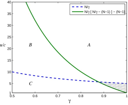
0.5 0.6 0.7 0.8 0.9 1 1 5 10 15 20 25 30 35 40 γ A C B u/c N/γ N/γ [ N/γ − (N−1) ] − (N−1)
Figure 1 Conditions (13) and (15), with N = 5.
the optimal number of scrips to issue under the random scrip selection rule, a common selection rule considered in previous literature.
The monotonicity property (16), however, holds only under condition (15). Figure 1 depicts the condition. That is, in the area below the solid curve, due to monotonicity there is a threshold on the number of scrips (possibly infinity), below which always trade is an equilibrium strategy. The dashed curve in Figure 1 corresponds to condition (13) in Theorem 3. In the area above the dashed curve, no matter how many scrips are in the system, always trade is an equilibrium strategy. These curves partition Figure 1 into four ares. In area A, no matter how many scrips are in the system,
always trade is an equilibrium strategy. In area B, adding a scrip to the system decreases every
player’s total discounted value except that of the player with the additional scrip; however, we know that each player’s total discounted value remains positive and thus no matter how many scrips are in the system, always trade is an equilibrium. In area C, adding a scrip to the system decreases every player’s total discounted value except that of the player with the additional scrip; in this case, there is a threshold (possibly infinity) on the number of scrips above which at least one of the player’s total discounted value is negative. This leaves the shaded area depicted in the
figure not covered by theoretical results. Later in Section 4.1, we conduct a numerical study on the shaded area, which indicates that although the monotonicity property (16) does not hold, it is very likely that there still exists a unique upper bound on the number of scrips.
Theorem 2 in the previous section, combined with the upper threshold on the number of scrips implied by Proposition 4, gives the following main result of the paper.
Theorem 4. In a scrip system with N players and at least N scrips, for any given set of model
parameters such that u c ≥ 2(N− 1) √ N2+ 4N− 4 − N , or γ≤ N (√N2+ 4N− 4 − N) 2(N− 1) , (19)
there is an upper bound ¯R (possibly infinity) on the number of scrips, below which always trade is an equilibrium strategy under the minimum scrip selection rule, and the system optimal social welfare is achieved in the game. Furthermore, the upper threshold ¯R increases with γ and u/c.
Sufficient condition (19) covers the area to the left and above of the intersection between the solid and dashed curves in Figure 1. As we will demonstrate in numerical studies in Section 4.1, the monotone threshold structure presented in Theorem 4 likely holds even without these conditions being met.
4.1. Shaded Area
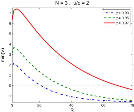
We do not have theoretical results when conditions (13) and (15) are both violated, depicted by the shaded area in Figure 1. Therefore, we conducted numerical studies to check the structure of the value function in its minimum recurrent state. In particular, we take a grid of values for u/c and γ in the shaded area when N = 3,2 and we see how the minimum value function value (over
recurrent states) changes with increasing R. We observe that in every case, the value function is unimodal and therefore monotonically decreases as R increases to be large enough. Figure 2 depicts one such example.
The findings indicate that when condition (15) in Proposition 4 is violated, a player’s value function does not always decrease monotonically with more scrips given to others. On the other
3 20 40 60 78 −1 0 1 2 3 4 5 6 7 R min(V) N = 3 , u/c = 2 γ = 0.93 γ = 0.95 γ = 0.97
Figure 2 The non-monotone, unimodal structure of the value function in its minimum recurrent state.
hand, in our numerical examples, it always first increases when the number of scrips R is small, and then decreases. Therefore, as long as the minimum value function over recurrent states is positive at the smallest scrip number R = N , there still is a unique upper bound (possibly infinity) on the number of scrips, below which the value function is positive in all states. If so, the threshold on the number of scrips in the system increases with γ and u/c, even without the necessity of condition (19).
The following result indicates that when R = N the value function is indeed positive in all recurrent states.
Proposition 5. Assume R = N and
u c ≥ N γ [ N γ − (N − 1) ] − (N − 1) . (20)
The value function V that solves the recursive equations (10)-(12) under the minimum scrip selec-tion rule is positive in all recurrent states.
4.2. Random Scrip Selection Rule
As mentioned above, there is a possibility that a different service provider selection rule may permit a greater number of scrips than the minimum scrip selection rule. We showed that for a given number of scrips in the system, the minimum scrip selection rule achieves the maximum social welfare, but it could be possible that with more scrips in the system, a different service provider selection rule still guarantees that no player will default, and therefore may outperform the minimum scrip selection rule at its threshold of fewer scrips. Here we analyze the optimal number of scrips to issue under the random scrip selection rule, a common selection rule considered in previous literature.
For a scrip system following the random scrip selection rule, where a player is selected as the service provider uniformly at random, the function V satisfies the following recursive equation,
V = T V , (21) in which (T V )(r, 1) = { γ N ∑ j′V (r, j′) , r1= 0 u +N (Nγ−1)∑j′∑i̸=1V (r− e1+ ei, j′) , r1> 0 , (22) and (T V )(r, j) = { γ N ∑ j′V (r, j′) , rj= 0 −c N−1+ γ N (N−1) ∑ j′ ∑ i̸=jV (r− ej+ ei, j′) , rj> 0 . (23)
Similar to Proposition 4 for the minimum scrip selection rule, the following result holds for the random scrip selection rule.
Proposition 6. Assume value function V satisfies recursive equations (21)-(23) for a scrip
system with the random scrip selection rule, and value function ¯V satisfies recursive equations (21)-(23) for a system with the same parameters except with R + 1 scrips. Further, assume that
u c ≤
N
γ − (N − 1) . (24)
For any nonnegative integer vector r such that ∑jrj= R and any player index j and k̸= 1, we
have
¯
∑ j ¯ V (r + e1, j)− ∑ j V (r, j)≤cN γ . (26)
Property (25) is a monotonicity property for value functions across different state spaces, and states that if we inject one more scrip in the system, every player, other than the one who receives the scrip, is worse off (measured by the value function). For the one who does receive the additional scrip, while it is intuitive that the person is better off, property (26) states that the benefit is, in fact, upper bounded. The proof is similar to that of Proposition 4 and is presented in the Appendix. For similar reasons as discussed above for the minimum scrip selection rule, property (25) implies that there is a threshold (possibly infinity) on the number of scrips in the system, above which the value function at some state may become negative. Numerical studies similar to those described in Section 4.1 suggest that conditions (13) and (24) are sufficient, but not necessary, for the threshold structure to hold.
Interestingly, therefore, both the minimum scrip selection rule and the random scrip selection rule permit a threshold number of scrips in the system (possibly infinity), above which the system crashes. Depending upon the system parameters u, c, N , and γ, numerical results show that sometimes the minimum scrip selection rule permits at least as many scrips as the random scrip selection rule; in this case, the minimum scrip selection rule is the preferable service provider selection rule for the scrip system because it provides a greater social welfare. For other parameters, though, the random scrip selection rule permits more scrips than the minimum scrip selection rule, and in some cases the difference is enough to cause the random scrip selection rule to outperform the minimum scrip selection rule in terms of social welfare. Depending on the system parameters and application, the system designer may choose to compare the performance of the minimum scrip selection rule and the random scrip selection rule before creating the scrip system. Since both exhibit a threshold property on the number of permissable scrips in the system, this should be relatively simple to do.
5.
Conclusion
In this paper we study design issues for managing a scrip system in a stochastic setting. In partic-ular, in each period one player becomes a service requester and receives positive utility if another
player is willing to provide the service in exchange for a scrip. We first show that a central planner would always prefer a trade of scrip for service to occur and would select the player who has the least number of scrips to be the service provider.
In a stochastic game setting with the absence of a central planner, such a system optimal solution can be achieved in equilibrium when the time discount factor is high enough or when the benefit of service is high enough compared with the cost to the service provider. When the time discount factor, or ratio between the benefit and cost of service, is not that high, we show that when using the minimum scrip selection rule or random scrip selection rule there is an upper bound on the number of scrips that are allowed in the system, above which some players may decide to default and exit the game when their scrip stock becomes low. Furthermore, this upper bound increases with the time discount factor as well as the ratio between the benefit and cost of service.
From a system design point of view, our results demonstrate that, assuming players follow the minimum scrip selection rule, the number of scrips in the system should be at the upper bound, and all players have the incentive to trade scrip for service whenever the service requester has at least one scrip. We also analyzed a commonly used service provider selection rule, the random scrip selection rule, and showed similar threshold results as the minimum scrip selection rule. This makes it simple for the system designer to compare the performance of the minimum scrip selection rule and the random scrip selection rule and choose the rule that results in the greatest social welfare. There are a number of possible extensions to our paper that deserve further exploration. The most notable one is that preferences are not homogeneous among players. For example, some players may value the service more than others, or providing service may cost some players more than others. Similarly, the benefit and cost of service may change over time or be stochastic. We suspect that the reason why our system does not experience a market crash when there are too few scrips, as observed in some applications, is a result of our current assumptions on the homogeneity of utilities across players and over time. Future work will hopefully provide us with more insights on this type of market crash. Another extension that is worth studying is that the price of service
may not be fixed at one scrip, but is instead determined according to the scrip distribution among players.
Endnotes
1. When too many scrips are issued and a player i’s scrip stock is running low, other players may refuse to provide service to player i in exchange for a scrip, in order to avoid player i’s bankruptcy. We do not study such complex strategic plays. Instead, from a system design point of view, our results justify simply upper bounding the number of scrips in the system to guarantee that trade always occurs.
2. Since the state space grows exponentially with N , which poses significant computational chal-lenges, we did not check for higher values of N .
Acknowledgments
We thank Saed Alizamir for very valuable comments and suggestions, which led to improvements in the paper. This research was partially supported by NSF Contract CMMI-0758069 and Masdar Institute of Science and Technology (MIST).
Appendix
Proof of Proposition 1
In this proof we show that starting from a functionJ that satisfies conditions (C1), (C2) and (C3), ΓJ also satisfies them. First note that function J0= 0 for all r (obtained from J0= 0 for all (r, j)) satisfies all
these conditions.
Condition (5) forJ implies
(u− c) + γ
Nmmax:m̸=lJ (r + em− el
)≥ γ
NJ (r) ,
which further implies
(ΓJ )(r) = Nr(u− c) + γ N [ (N− Nr)J (r) + ∑ l:rl≥1 max m:m̸=lJ (r + em− el) ] . (27)
More generally, we re-write the above Bellman equation as
(ΓJ )(r) = Nr(u− c) + γ N [ (N− Nr)J (r) + ∑ l:rl≥1 max ξ∈∆l J(r +∑ m ξmem− el )] , (28)
where set ∆l={ξ : ξl= 0, ξm≥ 0∀m ̸= l, ∑
mξm= 1}. The formulation allows the service can be provided
and paid for in fractions. We will show later that when r is integer, such a generalization does not change anything – the optimal selection ξ still guarantees that one particular player may be selected.
1. Condition (C1)
We first show that condition (3) holds for ΓJ in (28). That is, (ΓJ )(r) = (ΓJ )(r′). Note that
(ΓJ )(r′) = Nr′(u− c) + γ N (N − Nr′)J (r′) + ∑ l:r′l≥1 max ξ∈∆l J(r′+∑ m ξmem− el ) . Obviously, Nr= Nr′, andJ (r) = J (r′) due to (3). Considering the following cases.
• l ̸= i, j. For m ̸= i, j, we have J (r + em− el) =J (r′+ em− el) since (r + em− el)i= (r′+ em− el)j and
(r + em− el)j= (r′+ em− el)i. Furthermore, we have J (r + ei− el) =J (r′+ ej− el) andJ (r + ej− el) =
J (r′+ e i− el). Therefore, maxξ∈∆lJ (r + ∑ mξmem− el) = maxξ∈∆lJ (r ′+∑ mξmem− el).
• ri≥ 1 and l = i. For m ̸= j, we have J (r + em− ei) =J (r′+ em− ej). Furthermore, we haveJ (r + ej−
ei) =J (r′+ ei− ej). Therefore, maxξ∈∆lJ (r +
∑
mξmem− el) = maxξ∈∆lJ (r
′+∑
mξmem− el).
• rj≥ 1 and l = j. The same logic as in the previous case reveals maxξ∈∆lJ (r +
∑
mξmem− el) = maxξ∈∆lJ (r
′+∑
mξmem− el). Overall, we must have ∑l:r
l≥1maxξ∈∆lJ ( r +∑mξmem− el ) =∑l:r′ l≥1 maxξ∈∆lJ ( r′+∑mξmem− el ) , which implies the result.
2. Condition (C2)
We assume (4) holds forJ (r) and show that it must also hold for (ΓJ )(r). First, we show the following lemma.
Lemma 6. Assume r(1)l ≥ 1 and r
(2) l ≥ 1. λ max ξ∈∆l J(r(1)+∑ m ξmem−el ) +(1−λ) max ξ∈∆l J(r(2)+∑ m ξmem−el ) ≤ max ξ∈∆l J(λr(1)+(1−λ)r(2)+∑ m ξmem−el ) .
Proof: Denote ξ1, ξ2 and ¯ξ to represent the optimal indices for the three maximization problems in the
inequality. We have J(λr(1)+ (1− λ)r(2)+∑ m ¯ ξmem− el ) ≥ J(λr(1)+ (1− λ)r(2)+∑ m ( λξ1m+ (1− λ)ξ 2 m ) em− el ) ≥ λJ(r(1)+∑ m ξ1mem− el ) + (1− λ)J ( r(2)+∑ m ξm2em− el ) ,
The right hand side of equation (28) is the summation of concave functions, which is still concave. Now we argue that the generalization in (28) to allow non-degenerate ξ does not increaseJ for integer vector r. Consider any vector r with ri> rj. Denote d = ej− ei. Symmetry (3) impliesJ (r + (ri− rj)d) =
J (r). Further, concavity (4) implies that J (r + αd) is concave in α, and therefore J (r + αd) ≥ J (r) for any
α∈ [0, ri− rj].
Now assume integer vector r with rjbeing the smallest component in r except possibly rl, and ri≥ rj+ 1. Consider two vectors ¯ξ and ˆξ such that they are the same, except in two components: ¯ξi> 0, ˆξi= 0, and
ˆ
ξj= ¯ξi+ ¯ξj. Denote ¯r = r + ∑
mξ¯mem− el, and ˆr = r + ∑
mξˆmem− el. Since ri≥ rj+ 1, we have ¯ri≥ ¯rj, and ¯
ri− ¯rj≥ 1 + ¯ξi− ¯ξj, and therefore ¯ξi∈ [0, ¯ri− ¯rj]. Together with ˆr = ¯r + ¯ξid, we haveJ (ˆr) ≥ J (¯r). Following
the same logic for any ri> rj, we obtain that the value of maxξ∈∆lJ (r +
∑
mξmem− el) is achieved when ξ is zero in all components except smallest in r. If there is more than one smallest component in r, symmetry further implies that we can select one of them for a degenerate ξ. As a result, maxξ∈∆lJ (r +
∑
mξmem−el) =
maxm:m̸=lJ (r + em− el).
3. Condition (C3)
First, we show condition (5). From the previous proof, we know that forJ satisfying (C1) and (C2), when
rj> ri, we have J (r) ≤ J (r + ei− ej), which implies the condition automatically. Therefore we focus on
cases when ri≥ rj. Furthermore, player i must be the minimum scrip holder in r except j. Denote m∗l to represent the player that achieves maxm:m̸=lJ (r + em− el).
• rj≥ 2. In this case Nr= Nr+ei−ej= N . Therefore,
(ΓJ )(r) − (ΓJ )(r + ei− ej) = γ N ∑ l ( max m:m̸=lJ (r + em− el)− maxm:m̸=lJ (r + ei− ej+ em− el) ) ≤ γ N ∑ l ( J (r + em∗l− el)− J ( (r + em∗l − el) + ei− ej ))
—|Ir| = 2. This means that Ir={i, j} and i is the unique minimum scrip holder in r except j. Thus for
each possible value of l, i is also the minimum scrip holder in r + em∗l− el; note that if ri= rjand l = k̸= i, j, then by (C1) we haveJ (r + ei− ek) =J (r + ej− ek) and we can choose m∗k= j to make this statement true. Therefore, condition (5) implies the following result:
(ΓJ )(r) − (ΓJ )(r + ei− ej)≤ γ N [ NN γ(u− c) ] <N γ(u− c) .
—|Ir| > 2. This means that player i is not a unique minimum scrip holder in r except j; in other words, another player(s) has ri scrips. For l = j, we know from (C1) thatJ (r + em∗j− ej) =J (r + ek− ej) for any player k̸= i with rk= ri. Thus, i is a minimum scrip holder in r + ek− ejand we can apply condition (5).
For l = i, i is the minimum scrip holder in r + ej− ei except j, so again we can apply condition (5). For
l = k̸= i, j with rk> ri, i is the minimum scrip holder in r + ej−ekexcept j, so again we can apply condition
(5).
Finally, for l = k̸= i, j with rk= ri, i is no longer a minimum scrip holder in r + ej− ek. In this case, if ri= rj, we know from (C1) that J (r + em∗k− ek) =J (r + ej− ek) and by choosing m∗k= j, we see that (r + ej− ek)i< (r + ej− ek)j and from (C1) and (C2) we haveJ (r + ej− ek)≤ J (r + ej− ek+ ei− ej). On the other hand, if ri> rj, we have|Ir+ej−ek| ≥ 3 and includes i, j, and k; since (r + ej− ek)j≥ 2 we know
condition (6) holds so we can apply condition (7). Putting all these cases together, we again have
(ΓJ )(r) − (ΓJ )(r + ei− ej)≤ γ N [ NN γ(u− c) ] <N γ(u− c) .
• rj= 1, ri> 1. In this case N = Nr= Nr+ei−ej+ 1.
(ΓJ )(r) − (ΓJ )(r + ei− ej) = (u− c) + γ N ∑ l:l̸=j ( max m:m̸=lJ (r + em− el)− maxm:m̸=lJ (r + ei− ej+ em− el) )
Following the exact same line of argument as above, we have
(ΓJ )(r) − (ΓJ )(r + ei− ej)≤ (u − c) + γ N ( (N− 1)N γ(u− c) ) <N γ(u− c) .
• rj= 1, ri= 1. In this case we must have maxm:m̸=lJ (r + em− el) = maxm:m̸=lJ (r + ei− ej+ em− el) =
J (r + ei− el), when l̸= i, j. And maxm:m̸=iJ (r + em− ei) =J (r + ej− ei)≤ J (r) = maxm:m̸=iJ (r + ei−
ej+ em− ei). As a result, (ΓJ )(r) − (ΓJ )(r + ei− ej)≤ (u − c).
Now we focus on showing condition (7). Again, from the previous proof, we know that for J satisfying (C1) and (C2), when rj> ri, we have J (r) ≤ J (r + ei− ej), which implies the condition automatically. Therefore we focus on cases when ri≥ rj. Also, note that in order for condition (6) to hold, we know that no players can have 0 coupons.
• rj≥ 2. In this case Nr= Nr+ei−ej= N .
(ΓJ )(r) − (ΓJ )(r + ei− ej) = γ N ∑ l ( max m:m̸=lJ (r + em− el)− maxm:m̸=lJ (r + ei− ej+ em− el) ) ≤ γ N ∑ l ( J (r + em∗l− el)− J ( (r + em∗l − el) + ei− ej ))
(1) There exists rk= 1. According to condition (6), all other players in Ir must have exactly ri scrip. For any player l̸= k, r + em∗l − el satisfies (6). Note thatJ (r + ej− ek) =J (r + ei− ek) since rj= ri. Thus by choosing m∗k= j, we have (ΓJ )(r) − (ΓJ )(r + ei− ej)≤ γ N ( (N− 1)N γ(u− c) ) <N γ(u− c) .
(2) rl≥ 2 for all l ∈ Ir. By choosing m∗l ̸= i when possible, r + em∗l − el always satisfies condition (6), which implies our result.
• rj= 1. Condition (6) implies that for all players l∈ Ir\ j, rl= ri. Therefore, i achieves maxi:i̸=jJ (r +
ei− ej), which has been shown earlier in the proof. Q.E.D.
Proof of Lemma 3: This result follows directly from the Folk Theorem for stochastic games (Theorem 9,
Dutta (1995)). In particular, we need to verify the following three conditions to invoke Theorem 9 in Dutta (1995):
1. Unichain selection rule guarantees that the set of feasible long-run average payoffs is independent of the starting state.
2. Each player’s long-run average min-max payoff needs to be independent of the starting state. Instead of considering the min-max payoff, we consider the “always refuse providing service” equilibrium strategy, which generates 0 long run average payoff, and therefore independent of the starting state.
3. The dimension of the set of feasible payoffs should be N . This condition holds because any single player
i can be ruled out from service, which creates a payoff vector that has a constant positive value for all players
except player i, who has value zero. The resulting N vectors, each corresponding to one player being ruled out, spanℜN.
Q.E.D.
Proof of Theorem 3: Start the value iteration algorithm (10)-(12) from ¯V (r, j) defined as,
¯ V (r, 1) = u r∑1−1 k=0 (γ N )k , if r1≥ 1 ; and ¯V (r, j) = 0 , otherwise.
Note that ¯V ≥ 0 in general, and, in particular, ¯V (r, 1)≥ u if r1≥ 1.
Next we verify that T ¯V ≥ ¯V ≥ 0.
1. When j = 1 and r1= 0 we have,
(T ¯V )(r, 1) = γ N ∑ j′ ¯ V (r, j′) = 0 = ¯V (r, 1) .
2. When j = 1 and r1> 0 we have, (T ¯V )(r, 1) = u + γ N|Υ(r, 1)| ∑ j′ ∑ i∈Υ(r,1) ¯ V (r− e1+ ei, j′) = u r∑1−1 k=0 (γ N )k = ¯V (r, 1) . (29)
3. When j̸= 1 and rj= 0 we have,
(T ¯V )(r, j) = γ N ∑ j′ ¯ V (r, j′)≥ 0 = ¯V (r, j) .
4. When j̸= 1, rj> 0, and 1̸∈ Υ(r, j) we have,
(T ¯V )(r, j) = γ N|Υ(r, j)| ∑ j′ ∑ i∈Υ(r,j) ¯ V (r− ej+ ei, j′)≥ 0 = ¯V (r, j) .
5. When j̸= 1, rj> 0, and 1∈ Υ(r, j), following (29) we have, (T ¯V )(r− ej+ e1, 1)≥ u. Therefore,
(T ¯V )(r, j) = [ − c + γ/N ∑ i∈Υ(r,j) ( ¯ V (r− ej+ ei, 1) + ∑ j′̸=1 ¯ V (r− ej+ ei, j′) ] /|Υ(r, j)| = [ − c + γ/N ∑ i∈Υ(r,j) ¯ V (r− ej+ ei, 1) ] /|Υ(r, j)| ≥[− c + (γ/N) ¯V (r− ej+ e1, 1) ] /|Υ(r, j)| ≥[− c + uγ/N]/|Υ(r, j)| ≥ 0 = ¯V (r, j) ,
in which the first inequality is due to ¯V ≥ 0, the second inequality due to (r − ej+ e1)1≥ 1 and therefore
¯
V (r− ej+ e1, 1)≥ u, and the last inequality from u/c ≥ N/γ.
Monotonicity and convergence of operator T imply that Vγ= lim
t→∞TtV¯ ≥ ¯V≥ 0. Q.E.D.
Proof of Lemma 4: Consider a scrip distribution vector rn0
n1n2, where exactly n0players have zero scrip, n1 players have 1 scrip, and n2players have more than 1 scrip; therefore n0+ n1+ n2= N . For n0≥ 1, under the
minimum scrip selection rule, from state (rn0
n1n2, j), the probability of transitioning into another state also
with n0 zero scrip players (including itself) is (n0+ n1)/N (this happens when either a zero scrip player or
a one scrip player becomes the type 1 player, j). Otherwise, with probability n2/N , the system transitions
into a state with exactly n0− 1 zero scrip players. For n0= 0, the probability of transitioning into a state
with one zero scrip player is n1/N , and the probability of transitioning into a state where there are no zero
scrip players is n2/N . This implies that when n0≥ 2 (and N ≥ 3), the system never transitions into state
(rn0
n1n2, j) from another state with fewer number of zero scrip players. In addition, since R≥ N, we must have
n2> 0 when n0≥ 1. That is, there is a positive probability when n0≥ 1 that the system transitions out of
state (rn0
n1n2, j) and into another state with one fewer zero scrip players. Starting from (r
N−1
01 , j), where the