Capactiy of single-hop communication links in wireless ad hoc networks

Capacity of Single-Hop Communication Links

in Wireless Ad Hoc Networks

by

Filip S. Antic

Submitted to the Department of Electrical Engineering and Computer Science

in Partial Fulfillment of the Requirements for the Degree of

Master of Engineering in Electrical Engineering and Computer Science

at the Massachusetts Institute of Technology

'kASSACtHSES

INSTIE

August2,200 OF TECHNOLOGY

August

2,2004 ~ste..ber oj8

Ojlj

JUL 1 8 2005

Copyright 2004 Filip S. Antic. All rights reserved.

LIBRARI ES

The author hereby grants to M.I.T. permission to reproduce and

distribute publicly paper and electronic copies of this thesis

and to grant others the right to do so.

Author

Department of Electrical Engineering and Compute; Science

2, 2004

Certified by_

/

.avi&H

./2

"tae in

/

.,e

~'eys~

i'

Supervisor

Accepted

by_

_

____

'---Arthur C. Smith

Chairman, Department Committee on Graduate Theses

Capacity of Single-Hop Communication Links

in Wireless Ad Hoc Networks

by

Filip S. Antic Submitted to the

Department of Electrical Engineering and Computer Science

August 2, 2004

In Partial Fulfillment of the Requirements for the Degree of

Master of Engineering in Electrical Engineering and Computer Science

ABSTRACT

This thesis defines the capacity of single-hop communication links in wireless ad hoc

networks as the transferable data rate over that link determined by the Shannon limit and

by the fixed modulation scheme and bit error rate. The resulting capacity formulas are

derived under the assumption of r-3

path loss and uniform, but random, distribution of

users. Rank of the link R is defined and included in the capacity formulas. After defining

link capacity, the improvement of capacity is studied when different network components

are implemented. These include successive interference cancellation (SIC), and multiple

antenna arrays at the transmitting and the receiving end of the link. These strategies are

then compared in terms of the dB improvement of capacity that they provide. Network

parameter NP is defined in order to characterize spatial reuse in the network, and optimal

network parameter is determined for maximizing link capacity in the process of dividing

the network single frequency channel into equally sized subchannels.

Thesis Supervisor: David Staelin

Acknowledgements

I would like to express gratitude to professor David Staelin for giving me

directions in my research and helping me shape this thesis. During my studies for Master

of Engineering degree over the past year, he was a perfect advisor: helpful, resourceful,

patient, and motivating. I enjoyed working under his supervision.

I would also like to express perpetual gratitude to my mother Danica and my future wife Zhenya for giving me endless support and understanding throughout my education. They made everything look easier and that is the reason why I dedicate this

thesis to them.

I would also like to thank my fellow students Siddhartan Govindasamy and Keith

Herring for working together on the project, discussing problems together, and helping

each other in developing ideas. I took pleasure in working with them.

In addition to them, I would like to express appreciation to Daniel Bliss and Andrew McKellips from Lincoln Labs for weekly audio conferences where they gave many useful comments on my work, clarifying many research issues. I would also like to thank Dan for taking his time to occasionally visit us at MIT and have insightful conversations with us.

Table of Contents

1. Introduction and Background Information 5

1.1. Overview 5

1.2. Related Work 6

1.3. Attenuation Model Assumptions

9

2. Metric Definition 13

2.1. Significance of Metric

13

2.2. Requirements 13

2.3. Rank and Network Parameter

15

2.4. Formula Derivation

18

3. Successive Interference Cancellation

29

4. Multiple Antennas 35

4.1. Motivation 35

4.2. Assumptions

36

4.3. Capacity Improvement

43

4.4. Single User Exception

51

4.5. Antenna Array Spacing

52

5. Optimal Spatial Reuse

55

5.1. Overview 55

5.2. Problem Definition

56

5.3. Results 59

Chapter 1:

Introduction and Background Information

1.1. Overview

This thesis is a part of a larger project underway in the Remote Sensing and

Estimation Group (RSEG) of RLE at MIT. In this age of increasing use of radio spectrum

for mobile communication, many research attempts (both theoretical and practical) were

made to examine and find the best implementation of ad hoc wireless networks for wider

use. Some of those attempts will be mentioned in later parts of this thesis. However,

RSEG is concentrating on the problem posed by the increasing density of ad hoc wireless users in space, frequency and time, the foreseen future crowding problems. This group

plans new systems for wireless ad hoc networks, including details about their

infrastructure.

The systems they are analyzing include, among other things, protocols especially

designed for this purpose. The current versions of system protocols include reservation

signals for data channels, which are sent or not sent over side channels, beacon signals,

and other versions. The system designs also include proposals for use of multiple

antennas for blind signal separation and eliminating the signals that are discovered as interferers at the receiver's end of the data links Another purpose of multiple antennas will be to enhance the data rate communicated over the network links by directing the antenna gain in the direction of the user on the other end of the link, and decreasing the antenna gain in the directions from which the concurrent interfering signals come. This is the strategy of (partially) nulling the interfering signals and at the same time peaking up on the direction of the link, and is examined by simulations in this thesis.

This project is currently in its theoretical phase and, as a consequence, all results presented in this thesis are derived from simulations. The main purpose of this thesis was to find the theoretical limits to the data rate each user can get for himself in a crowded

the Shannon's binary channel capacity formula, and the data rate achievable when the

modulation scheme and tolerable bit-error rate were fixed for all users in the network.

These theoretical limits and the information concerning how various components

of the system influence these theoretical limits will help further theoretical and practical

work on the larger project. Although the results depend on certain assumptions, for

example the attenuation model and multi-antenna array constraints, the results can be

easily modified as one assumes different things. For example, once the equipment now

being developed by RSEG collects data concerning signal attenuation, a new different

model can be discovered and incorporated in this work.

1.2. Related Work

Ad hoc wireless networks have been subject of many research efforts and some significant results have been achieved. The work of Gupta and Kumar [1] has shown that

the transferable bit rate in multihop scenarios is

(n) =

x l

for randomly

In xlo gn

chosen source and destination users, where n is the number of users of the network in a

fixed area,

is the number of bits per second that each user alone can transfer, and the

order

0

is

defined

by

the

equivalence

relation

f(x)

E(g(.X))

f(x)

O(g(x))A g(x)

O(f(x)).

Their result is valid for multihop

communication, but it depends on the singlehop transferable data rate W. This thesis

complements the result [1] of Gupta and Kumar in the sense that it determines W from

various system components.

Multiuser detection is an important part of the design of future ad hoc wireless

network systems, because it allows greater tolerance of receiver towards interference

coming from other users in the network. Verdu did pioneering work in this field. In one

of the first papers [2] he determined asymptotic bounds of multiuser detection method

efficiency. Later, in [3], he and V. Poor described single-user detectors for multiuser

channels, and determined optimal detectors under several different specific channel

conditions such as power level of interferers and length of spreading codes of CDMA

signature waveforms. Lupas and Verdu went on in [4] to design a linear multiuser detector in a synchronous CDMA channel and prove that its performance is close to that

of the optimum multiuser detector. This result was important since the computational

complexity of the proposed linear detector was liner in the number of users, which made

it applicable in real systems. Verdu and Lupas also proved in [4] and [5] that linear

detectors are, near-far resistant in synchronous and asynchronous CDMA channels and

that result implied that linear detectors can be used in wireless communications since

they could combat the large range of interfering signal power levels which is inherent in

wireless systems. However, these papers did not consider blind multiuser detection,

which does not require beforehand knowledge of signature waveforms. Honig, Madhow

and Verdu considered this issue in [6] and proposed an adaptive linear multiuser detector

which could do blind detection. In summary, this series of research efforts made huge

progress in multiuser detection in wireless systems. The results of these mentioned papers

are the foundation of successive interference cancellation, which is one of the methods

whose contribution is evaluated in this thesis.

Other methods that can boost the data rate of a single link in an ad hoc network

include usage of multiple antennas. Research done on space-time coding is summarized

in [7] and [8]. Space-time coding is beyond the scope of this thesis, but can be examined in the future. There have also been efforts to determine the theoretical limits of Shannon

capacity for multiple input multiple output (MIMO) systems, which are summarized in

[9]. The loss of MIMO system capacity in the presence of environmental hindrances is

examined in [10]. Papers [ 11] and [ 12] present some experimental results in this area for

frequencies near the PCS frequency allocation (1790MHz).

Ad hoc wireless networks imply large interference between users, and multiple antennas can be used to detect and subtract interfering signals. [9] provides an overview of achievements in this area. In order to get good results, one must assume some

knowledge of the MIMO channel, both from the transmitter and receiver's point of view.

That includes, the knowledge of either the exact state of the channel gain matrix, or the distribution of the matrix's coefficients, as well as the noise distribution. Those are big assumptions to make, but on the other hand this method is useful for detecting not only one signal among its interferers, but all of the signals received, one by one. The last

signal detected then has the strongest data rate (since the other signals are detected and

subtracted beforehand). This method for our purpose is only important as a form of

successive interference cancellation, looked at in this thesis. In contrast to this method,

this thesis also contains examination of multiple antennas used for a different purpose

-nulling the interferers. Instead of, or in addition to, detecting and subtracting the

interfering signals, one can use the antenna inputs to boost the SINR of the receiver by

choosing the best linear combination of inputs. More on this is presented in chapter 4.

In MIMO systems, the receiver needs to know the state of the channel gain matrix. The transmitter achieves that by sending the training signals for a period of time to the receiver before actually sending the data packet. The process is explained in [16]

together with the recommended length of the training data package.

In addition to [1], there have been more papers on network capacity defined in the

similar manner. Mostly their definition of network capacity was the aggregate data rate

that could be transferred between randomly chosen users in the network under an

arbitrarily defined protocol. In [13], a three-dimensional ad hoc network was examined,

under a time division protocol and multihop routing. Although the bounds were correct in

the limit, they were only correct up to a multiplicative constant. That is why this thesis is

complimentary to the bounds determined for multihop routing if we want to estimate the

achievable data rate at a more exact level.

One more thing that this thesis tries to do is determine how different components of network infrastructure influence achievable data rate (both on the link and on the network level). Extensive work on this subject has already been done in A. Goldsmith's group at Stanford. The paper [14] describes capacity regions of the network data rates when different network designs are used. It is notable that multihop data transfer brings

large improvement over singlehop, and spatial reuse as well, while power control does

not bring much improvement. The last method examined in [14] was successive interference cancellation (CIS), which in combination with multihop and spatial reuse achieves the greatest capacity region. This thesis, on the other hand, examines the use of multiple antennas for partial nulling of interferers (chapter 4) and makes further

Protocols for multihop routing are the next issue in finding the greatest data

throughput in the network. [15] examines several protocols and ranks them according to their performance. The results found there say that: power control does not help much in

data rate performance, CSMA/CA suffers from presence of weak links, a FIFO queuing

rule is suboptimal, and two contention based protocols examined had the best performance. The two protocols were both time-framed, with control signals preceding the data packets.

1.3. Attenuation Model Assumptions

One of the crucial assumptions of this thesis is polynomial path loss with respect

to transmitter-receiver distance. It is well known that in free space the intensity [ Wm-2 _]

of electromagnetic waves is proportional to r -2, where r is the distance from the

transmitter. However, near land, buildings and other objects the situation is much more

complicated. In such cases diffraction and reflection from various objects along the propagation path scrambles the field at the receiving point and the resulting field there is

no longer the result of a single path line-of-sight electromagnetic wave. The resulting

field very much depends on the position of all objects in the environment, buildings being

the most influential factor. However, one can still talk about the average dependence of

power on distance, and many experiments have confirmed that, on average, power is proportional to r -a for some value of a. In [17] we find that a is usually between 2 and 4, and on average a=3.8. That is why in this thesis the simulations and results are presented for case of a =3.8 as that is the most referenced value for propagation constant:

P = A r -, where a =3.8.

(1)

The justification for choosing polynomial path loss comes from several different experimentally developed path loss models. The first one is the Okumura-Hata model [18], where Hata has derived an equation based on numerous path loss curves that Okumura has measured in wide variety of conditions. Actually, there are several

equations, one for each of the following: large city, medium and small city, suburban

area, and open area. All of them contain the dB path loss factor in the equation:

Lpu(dB)= ... + [44.9-6.55

logohb(m)]

loglor(km) + ... ,

(2)

where r and hb are distance from the base station and height of the base station. The result

is polynomial path loss with respect to r, as claimed above. The only problem with this

model is that it has been derived from measurements with hb ranging from 30m to 100m, which are antenna heights larger than usual in ad hoc wireless networks. However, I have

mentioned it here because it is the most accurate and complete experimental path loss

model for urban environments in existence today.

Other researchers have also arrived at polynomial average path loss. In [19] we

can find the results of a field experiment in the city of Helsinki, Finland. The researchers determined that at frequency 5.3 GHz path loss fits the polynomial model for both

line-of-sight and non line-line-of-sight cases. For line-line-of-sight the attenuation coefficient oscillates

from value 1.4 to value 3.5, where value 1.4 is actually less than in the free space case, which is equal to 2. The reason for this is because a street can sometimes act as a waveguide and carry the power of electromagnetic waves over longer distances. On the other hand, for non-line-of-sight cases the attenuation coefficient oscillates between 2.8 and 5.9, again around the value 3.8 used in this thesis. These experiments have been conducted with antennas of height 4m, 12m, and 2.5m, all of which being below rooftops, which makes the results more applicable to our purpose and ad hoc networks.

In addition to Okumura-Hata, there have been other empirical models. One of

them is the COST-Walfisch-Ikegami model, which derives the path loss equation by

taking into account the dominant role of multiple diffractions of waves over the rooftops of buildings [20]. This model also considers the width of the streets where the receiver is located and has a fine estimate of the roof-to-street segment of the signal path. However, what is important for us is the polynomial path loss that again appears in this model. For line-of-sight cases the path loss of the signal contains the factor:

which corresponds to the attenuation constant 6a=2.6. In the non-line-of-sight cases the

path loss contains the factor:

38 log r(km), Htx > Hr

(4)

t38-15

Htx

Hroof )logr(km),

Htx

Hroof

where r, Htx, Hrx and Hroof are distance from receiver to transmitter, transmitter antenna

height, receiver antenna height, and rooftop height, respectively. The corresponding

value of attenuation constant here is a =3.8 minus a correction factor for the case when

transmitter is below the rooftops. From here we conclude that this model supports the

assumption of polynomial path loss and the choice of attenuation constants for the

simulations and experiments.

Even though on-average path loss can be considered polynomial, there is evidence to believe that this assumption is overly simplified. If we look at the research results in the area of designing microcellular telecommunications systems in big cities, we find that the power attenuation greatly depends on the street pattern. In the paper [21] the

boundary of regions with fixed path loss assumed a diamond shape in the rectangular

parts of the streets of Boston, as opposed to circular pattern one would expect from

polynomial path loss with respect to distance. The corners of the diamond shaped figure

extended in the direction of the streets on which the transmitter was located, which means

that the attenuation was stronger across the building blocks and weaker along the streets. This effect was evident for the frequencies on which the research concentrated, 2GHz and

6GHz, which also happen to be very close to the candidate frequencies for allocation to ad hoc wireless networks studied in this thesis (2GHz and 5GHz). The same paper also examines pattern of attenuation in the downtown Boston area, which has curvilinear

instead of rectangular street pattern. In this case the boundary figure assumes an irregular circular shape, supporting evidence for the polynomial path loss model.

There is another example why polynomial path loss could be considered

excessively simplified. In [19], experiments were conducted at 5.3GHz, again very close

to the candidate frequency for application of ad hoc networks. One of their observations

was the dramatic change in path loss when the receiver turned around the corner from the street where the transmitter was located to the street perpendicular to it. The path loss pattern was polynomial in the first street and also in the second street, but between them there was a sharp cutoff of 26dB.

This effect again proves that the street pattern greatly influences the path loss.

However, the simplification of putting complicated multiple diffractions and refractions

along streets and buildings into just one constant a, was enough to decide to neglect

these objections for the time being. The next research step could be incorporating street geometry into the simulations and path loss model. One approach could be to include

another constant or random variable to supplement a in description of propagation loss,

and another one could be to distort the Euclidian space where the users and interferers are located in order to accommodate street shape dependence. In such research attempt users that are located along the same street could be considered closer than their actual

distance, and the users isolated from each other with many obstacles could be considered

farther than their actual distance; just so they all fit into the r -a attenuation model used

Chapter 2:

Metric Definition

2.1.

Significance of Metric

We would like to be able to compare two given infrastructures of an ad hoc wireless network. The ad hoc network is always given to us, because we cannot change

the geographical distribution of users or the physical characteristics of the environment.

However, what we can do is design the infrastructure of the ad hoc network so that the

owner of the network is maximally satisfied. The infrastructure includes but is not limited

to the antenna characteristics, blind signal separation methods, and the protocol that the users have agreed to use while transmitting data over a link. All these characteristics can be changed to improve the satisfaction of the users in the network, but they also have

their cost of implementation. That is why we need a tool to predict how much exactly

each change in every infrastructure design detail contributes to the total performance of

the network. We need a scale on which we could rank the overall performance of

different infrastructures for the same ad hoc network.

2.2. Requirements

The most natural metric to use for communication systems is the data rate of the users, since data transfer is the basic purpose of such systems. In this thesis I examine the

data rate that can be transferred over one link, from the transmitter to the receiver, with

no consideration of multihop strategy. The basic model of transfer that I consider is one transmitter, one receiver, and other users, whose transmissions interfere at the receiver with the desired signal coming from the transmitter. The interference can then either be eliminated by successive interference cancellation, or simply added to the thermal noise and considered as additional noise.

There are two different ways that we can use to determine transferable data rate

over a link. One is to use Shannon's binary channel capacity, which would give us the

maximum data rate over the link. However, even though this limit is a useful value to

know, it is not practically achievable in wireless systems, since that would require infinite

delays while recovering data. That is why I considered another way of determining data

rate over a link. The other approach would be to assume a fixed modulation scheme and

fixed bit-error rate that can be tolerated, and calculate the data rate from there. This

second approach is closer to practical implementation than taking the Shannon's limit,

but, nonetheless, both approaches for calculating data rate are considered in this thesis,

the first one as the absolute limit, and the second one as practically achievable data rate.

A higher data rate makes the system more appreciated, but we must consider the

tradeoffs as well. A higher data rate is likely to increase the cost of system

implementation, and the cost is distributed over different components of the system. That

is why we would like to have a way of determining how much each component of the

system influences the data rate in an average link in the network. When one has such

information one can decide which component of the system is best to invest in, in order to get maximum improvement of the data rate at minimum total cost.

In the later part of this chapter, I present the equation that calculates the data rate

over a link as a function of different system components characteristics. That equation

exactly serves the goal of making transparent which parts of the system are best to invest

in for achieving optimum data rates on communication links in the network. In chapters 3

and 4 I describe how much successive interference cancellation strategy and multiple

antennas, which are some of the components of the system to consider, change the data

rate of links in the network through the equation defined in this chapter.

Before I derive the equation, let me emphasize some important assumptions about

the ad hoc wireless networks that we consider. The first one is that a network consists of

users distributed uniformly in a plane, but randomly, some of them being receivers and

others transmitters. A user can only be a receiver or a transmitter at a certain point of time, and both of them are distributed in the plane with the same area density. Data

transfer in such a network happens over single hop links between receivers and

considered as interference at all receivers except for the one receiver that is expecting the

signal. All signals attenuate according to the polynomial attenuation model described in

the previous chapter, with attenuation constant a. These assumptions explain most

features of the network, but in order to get a sense of what is the data rate on a link, we need to know the link length relative to the distances to the interferers in the area.

2.3. Rank and Network Parameter

Rank of the link is a measure of relative distance from the transmitter to the

receiver, relative to the distances from the receiver to the other transmitters in the area.

The exact definition is as follows:

In a link of rank R the receiver is listening to the Rh closest transmitter, while all other

transmitters are considered to be interferers to that receiver.

Since all transmitters are assumed here to have equal power, the Rth closest transmitter is

also the Rth _{strongest if all antennas are isotropic.}

Rank in combination with knowledge of area density of transmitters (p) is all the

information that we need about the geographical distribution of transmitters (both desired

and interfering) around the receiver, for R > 2. For R = 1 you might use the network parameter, which is defined a few paragraphs below. One can also determine roughly

what is the link length ( r ) from the knowledge of rank and area density of transmitters in

the area (for R 2):

r2

R

P R(5

I R

~r-~~~~~

,

of

(5)

where p is equal to #transmitters/m 2 in the network.

From this connection between r and R, and the fact that power of the received

signal has a polynomial dependence on r, we can derive a further connection between R and the signal power level at the receiver. This fact is going to be used in the derivation

of the equation for data rate over a link of rank R later in this chapter. For R = 1 formula

(5) cannot be used for determining the power level of the signal at the receiver, and in that case other methods, such as using the network parameter, need to be used for calculating the data rate over the link. Other information that we need in order to find the data rate over the link include the interference level at the receiver, which is equal to the

sum of all individual signal powers coming from interfering transmitters surrounding the

receiver. For calculating individual interfering signal powers we can still use formula (5)

in combination with the polynomial attenuation model, but only for rank of interferer

R > 2. The largest interferer, with rank R = 1, does not obey equation (5) and other

methods need to be used in order to estimate its power level.

Rank was defined above for a single link, but we can also talk about rank of a network, or part of a network. Here is the definition:

In a network, or part of a network, of rank R, all links have rank R.

This is a loose definition, since strict application in practice would mean that sometimes two or more receivers listen to the same transmitter at the same time, because

the Rth _{closest transmitter from one receiver can at the same time be the R}th _{closest from}

another receiver. Networks of different rank are visually distinguishable, as shown on the images below. All links in these images have the same rank, so the overlapping can be noticed, which should not happen in practice. However, the idea here is to get a sense of how long are the links in the network relative to the distances between users in a network

/ / -.

kn'

<

/.

x ~

f/

1

Figure 1: (a) Network of rank R = 1; (b) Network of rank R = 5; (c) Network of rank R = 10; (d) Network of rank R = 20.

In addition to rank, I consider another index value that characterizes link length relative to distances to interferers in the neighborhood. It is called the network parameter

(NP) and the definition is as follows:

NP

r

/,

->P

where r is the link length and p is the area density of transmitters around the receiver.

This definition is useful for rank R = 1 networks, because that is the only time the duality

relation (7) does not hold. One can easily derive the duality relation (7) from equations

(5) and (6).

NP_--

for R>2.

/TT

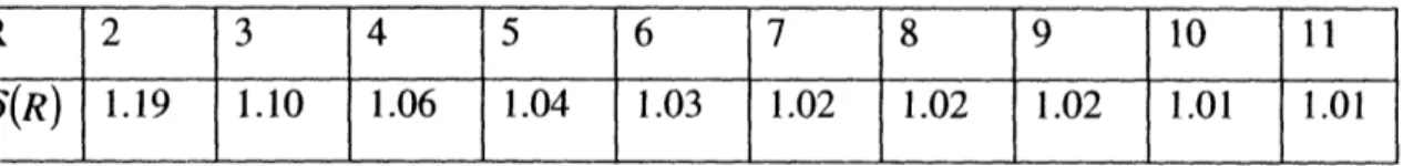
Some example values for NP are given in Table 1, with reference to rank values that are associated with them. Since the notion of rank is intuitively clearer than the notion of network parameter, I will use rank in all cases where I can, to describe the

distance of the transmitter from the receiver in a link, or a set of links. That will be the

case in chapters 3 and 4, while in chapter 5 I use the network parameter to describe the

optimum division of one frequency channel into many.

Table 1: Correspondence between values of rank R and network parameter NP for R > 2.

R

NP

2.4.

Formula Derivation

In the beginning of the chapter I mentioned two ways of calculating the bit rate that can be transferred over a link in the network. One approach is to evaluate Shannon's capacity limit, and the other approach assumes a certain bit error rate and a modulation

scheme, from where we can derive the bit rate over the link. Resulting bit rates from both

approaches are useful to know, but the first one is the absolute limit in the bit rate, while the second one would be more applicable to the actual systems.

The first approach, taking Shannon's bit rate, is simple; one just applies the

Shannon's capacity formula, bearing in mind how noise and interference, as well as the

signal power level at the receiver's end of the link, can be calculated from the parameters

of the system:

C = log

(1

+

SINR) [#bits

(8)

[ sec. Hz

where C is the limit on how many bits can be transferred over the link per second and per

Hz of bandwidth; and SINR is the ratio of signal power level and the sum of noise power

and total interference power in the same bandwidth.

In the other approach, one does not take the absolute Shannon limit, but instead

the limit under the assumption of a fixed bit error rate and a certain modulation scheme.

For example, in this thesis I have decided to concentrate on bit error rates at around 10-2,

which under the BPSK modulation scheme requires

at the level of approximately

No

5dB [22]. From here we can derive the dependence of achievable bit transfer rate in the

system on the SINR at the receiver's end of the link. The equation (9) at the end of this derivation presents the achievable bit rate normalized by time and bandwidth. The

starting equation is:

Esignal

Eb #bits

No EN+I

At B

where Eb is energy per bit, No is power spectral density of noise+interference, Esignal is the

total energy that the receiver gets during the time #bits are transferred to the receiver, and EN+, is the energy the receiver gets from thermal noise and interference during time At and over bandwidth B. The next step takes us to the bit rate capacity:

Eignal 1

At

#bits

At

N

W+

#bits

1=

= SINR-,

where SINR =

and C =

No

C

WN+I

At B

In the last two lines Wsig,,, and WN+I are power levels of the signal and the sum of noise

and interference at the receiver, respectively. The conclusion of this derivation is:

C=SINR

#its

E

O

sec- Hz

where SINR is the signal-to-interference+noise ratio at the receiver's end of the link. As

mentioned above, the value for

that is reasonable to assume is 5dB.

No

SINR

Formulas (8) and (9) both contain SINR as the key parameter, and that parameter needs to be estimated in order to get useful data rate equations from (8) and (9). There are certain assumptions that I use when estimating SINR. The first one is uniform distribution of transmitters in the area around each receiver. They are distributed randomly with area

density p [#users/m2 ], and the receiver is listening to only one of them, with rank R,

while the others are considered to be interferers to the receiver. All transmitters are

considered to transmit the same power with their antennas (Pr) and the power

Prec =

A

P,

where Prec,,

andPr

attenuation model, and r0 is a constant that connects Ptr and A. In addition to these

assumptions, I assume that all users in the network have isotropic dipole antennas, which have equal antenna gain in all directions in the plane. For now I consider that each user has only a single antenna, and in later chapters we can see what happens when one

provides each user with multiple isotropic dipole antennas.

An important assumption in addition to these is neglecting the thermal noise at the

receiver. The reason for this decision is simplification of the expression for SINR because when you do not have thermal noise in the equation, the parameters Ptr, A, and ro from (9)

appear in both the numerator and the denominator of the expression for SINR and they cancel out. Justification for this decision lies in the fact that one can always increase the power level of all transmitters in the network until the thermal noise is negligible in comparison to the level of interference.

The assumptions made in the previous two paragraphs make it possible to

estimate SINR as a function of numerical parameters describing the network. The

expression for the SINR (we could also call it SIR, since the thermal noise is neglected) is

fnow:

Wsignal A r(

SINR= Sig=

(1)

interf interf

where Wsig,,, and Wite are signal power level and interference power level, respectively. The first equality in (11) is completely true only when thermal noise is zero, but we

consider this equation to be an accurate enough approximation. In calculating the

expression for Win,ef I have tried two approaches, described below. Only the second approach gave a satisfying result, and that is why I use it for the derivation of the final formula for SINR.

Integration

The first approach was to integrate the power that the receiver gets from "blurred"

interferers in the network. In other words, I considered concentric rings centered at the

receiver, rings of width dr, radius r and area 2r. r dr, and assumed that in one such

ring there were dN = p 2nr- r dr users, which was an infinitesimal value, and did not

have to be an integer. Using infinitesimal values for power dWe = A. r- "dN, I could

integrate over area in the ring from the radius r to the radius r2in order to get total

interference power that comes from interferers between radius r, and radius r

:

r2

AWtr

(r, ,

)

dWiter

= A. r

dN

=IA r-

.p .2

rdr

A

p2

-

+2

r

for a > 2

A. p 22 Inrr,

for

o=

2

Total interference power level could be estimated from (12) when one substitutes

O and + oo for r and r2:

Winterf = AWinterf (0° ). (13)

However, it turns out that when you combine (12) and (13), the resulting interference power is infinite, Win,rf = oo, for both a = 2 and a > 2.

One could avoid infinite interference if only a > 2 is used and there are no

interferers in the neighborhood of the receiver within radius r,:

Wintef

=

AWitef (r

,

,

(14)

In this case the result for total interference

Wi,,ef

We( r, )=A .p. 2

_{WijpIof~ a-2}

_ra

1

_-2

(15)

The result (15) is better than infinity, but it is not good enough, because the value of r is then excessively important for determining the total interference.

In conclusion, integrating infinitesimal interference over the plane did not give

good results. Either the calculated interference was infinite, or it heavily depended on the

size of the "forbidden" neighborhood around the receiver. That is why I did not continue to use this approach in order to get the estimate for Wi,,,ef and SINR.

Monte-Carlo Experiments

The second approach for calculating W,,,f and SINR was to use Monte-Carlo trials. The actual formula for SINR that I used was:

SINR _ZA,,

(16)

where ri were all interferers in the network. In each experiment I used 1000 transmitters

randomly distributed in the network around the receiver, with area density

p [#users/m2 ]; one of them was the desired transmitter and all others were interferers. I

used only a =: 3.8 since a = 2 would in theory lead to infinite interference, which can be concluded from infinite upper integration limit in the second part of (12). For a = 3.8 the peripheral interferers do not contribute much to the total interference, so I distributed the transmitters in a square around the receiver and did not care about the edge effects. The total interference coming from outside of the square was estimated by using (14) and (15), and the resulting interference level was less than 0. I1%, a negligible amount.

One can see from (16) that the SINR does not depend on the power level of the transmitters, since A cancels out from the equation, and also does not depend on the

density of the users. The proof of the second claim is the fact that the scale of r and

ri also cancel out. In the further derivation of the SINR expression, I first cancel A from

numerator and denominator in (16), and then use (5) in order to eliminate the dependence

on r:

SINR

E ri

-SINR

_

SINR- R

_{) .}

₍₁₇₎

The expression (17) for SINR of the link contains two parts. The first one, R

,

captures the necessary information about the relative link length, following the definition

of rank of the link at the beginning of this chapter. The second part of (17) is a number

that depends primarily on the attenuation constant a and slightly on the link rankR,

while it does not depend at all on the area density of the users p (see (18)). The fact that the second part of (17) does not depend on p is very useful because it makes SINR a

function of only R and a, two very basic parameters.

In order to calculate the second part of (17) I used Monte-Carlo experiments. Here is the description of the experiment: in one trial I distributed 1000 interferers in a square area around the receiver, with the densityp [#users/m2]. I used different densities and the result did not depend on the choice. The attenuation constant was a = 3.8, and for

such an attenuation model the edge effects were negligible, so the summation ri ° ,

which in theory should include all interferers in an infinite plane, was well approximated by the 1000 users in a square around the receiver (the estimated error by using (14) was less than 0. 1%). The resulting formula for the SINR on the link was:

[SINR

(

R)-

where ywas a constant whose value was calculated to be y = 0.54731, and 6(R) was a

correction factor whose values are given in Table 2.

The constant y here is exactly equal to the estimated second part of the right-hand side of (17), the quantity we were looking for, but only in the case when all transmitters from the network were considered to be interferers and were included in the summation

rri . However, the definition of rank in this thesis says that for a link of rank R the

R'hclosest transmitter is considered to be the transmitter that the receiver is listening to,

and, thus, it should be excluded from the total interference level. In other words, we need

to exclude the transmitter from the summation

r,

, which corresponds to adding a

correction factor (R) in the formula (18). The values for the correction factor do not

change the result very much, at most by 19% when R = 2, and the effect practically loses significance very quickly as R grows. In the Table 2 the results from the experiment show how the correction factor changes with R, and one can see how it is a decreasing function of R and how its values approach 1 as R increases.

Table 2: The correction factor

6(R)

Formula

The expression (18) for SINR is simple and depends only on rank R of the link,

and implicitly on the assumption a = 3.8. It is valid for the case of randomly distributed

transmitters in the network with any density, with all transmitters having the same power

level and negligible thermal noise at the receiver's end. Both transmitters and receivers

the plane. Under all these assumptions, we have the expression for SINR and we can plug in that result into the two formulas for link capacity (8) and (9).

The capacity that was derived from the Shannon's limit is now

(19)

and the capacity that was derived after assuming error rate at

and BPSK modulation

scheme is

(20)

where R is the rank of the link (under the condition R 2); also y = 0.5473, (R) is

given in Table 2, E= 5dB = 10 , and 8 is the parameter that captures the effect of

No

successive interference cancellation and multiantenna nulling described in chapters 3 and 4. The value of/f for the time being is 1, but in the following chapters its value will be greater than 1, thus improving the link capacity.

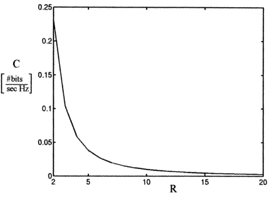
While we consideri = 1, we can use (19) and (20) to find the link data rate per

Hz and plot it as a function of R. The resulting plots are shown in Figures 2, 3 and 4.

|c=log 2(l+(R).

R)

[2)

sec Hz

1

C

#bits

se- Hz]

)

R

Figure 2: Capacity of a link in the network vs. rank of the link. This capacity corresponds to the Shannon's

capacity limit (data rate per Hz), calculated by formula (19). 0.

C

seaid

R

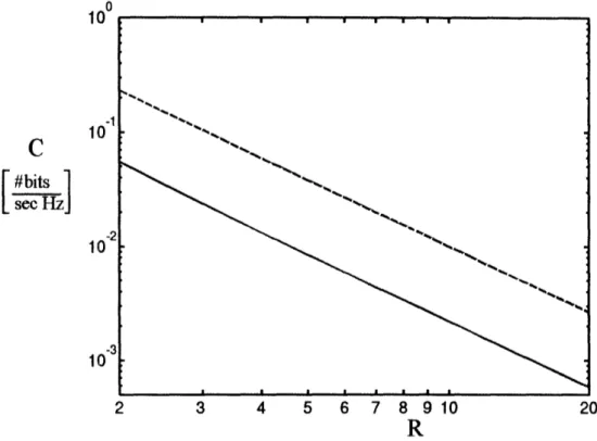
Figure 3: Capacity of a link in the network vs. rank of the link. This capacity corresponds to the data rate

per Hz, available under BPSK modulation scheme and with tolerable bit error rate 10- 2.The capacity is calculated by formula (20).

,,0 1 1

C

E

sec

R

Figure 4: Capacity of link vs. rank of the link, on a log-log scale. The top (dashed) curve corresponds to

the capacity in Figure 2, while the bottom (solid) curve corresponds to the capacity in Figure 3. The

difference between the curves is 6.2dB for R=2, and 6.4dB for R=20.

In conclusion, this chapter introduces the notion of rank of the link R and rank of the network, definition of the network parameter NP, and the connection between R and

NP. I used those definitions and under certain assumptions derived two types of link

capacity (given by formulas (19) and (20)) that depended only on the value of R and

implicitly on the attenuation constant a. The assumptions I made were: uniform

distribution of transmitters in the area, negligible thermal noise, polynomial path loss with attenuation constant a = 3.8, all users in the same bandwidth, and single isotropic dipole antennas at each user. Under those conditions, formulas (19) and (20) can be used with 8 = l, and once we introduce successive interference cancellation in chapter 3 and multiple antennas in chapter 4, the value for , can increase and we can see how much improvement each of these strategies bring to the link capacity, which is considered to be the base metric for measuring the performance of the system.

Chapter 3:

Successive Interference Cancellation

The isotropic dipole antenna case considered in the previous chapter was the base

for deriving the two forms of capacity formula, (19) and (20), but the capacity that is

determined this way is by no means the maximum achievable capacity. The factor in

formulas (19) and (20) captures the effects of using successive interference cancellation

(SIC) and multiple antennas. While multiple antennas will be discussed in chapter 4, in

this chapter I concentrate on SIC.

I do not go into the technical detail how the SIC is conducted, and do not determine what are its limits, but instead, I determine what are its effects on the capacity over a link in the wireless network. I assume that the description of the network is the

same as in previous chapters, and that formulas (19) and (20) correctly calculate link

capacity in the network. When no SIC is used, the factor/ is equal to 1, and all

interferers in the network are included in the total interference level.

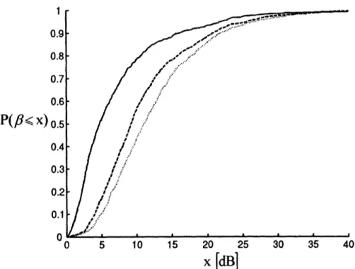
The SIC strategy that I assume here means that the receiver detects the interfering signals from the n strongest interferers, and subtracts them from the total interference level. As a consequence, SINR increases, which is then followed by the increase of the link capacity. The effect of SINR increase is captured in the multiplier/s, which is equal

to the ratio of the SINR after and before SIC. I plotted in Figure 5 the dB value of P

(improvement over its original value 1) vs. the number of subtracted interfering signals.

The source of these results were Monte-Carlo trials designed to measure the total interference, as well as interference after subtracting up to 20 strongest interferers from the total sum. Again, for each trial I used 1000 interferers distributed randomly in a square field surrounding the receiver. The attenuation model was polynomial with

a = 3.8, which made the edge effects negligible. I considered the thermal noise much

lower than the interference level, so I did not include it in the expression for SINR. There were 1000 trials for every number of cancelled interferers, and from them I determined the average value forfI as well as the standard deviation, which is plotted in Figure 5. I

also determined the average and standard deviation for the capacity values, which are

plotted in Figures 5-11.

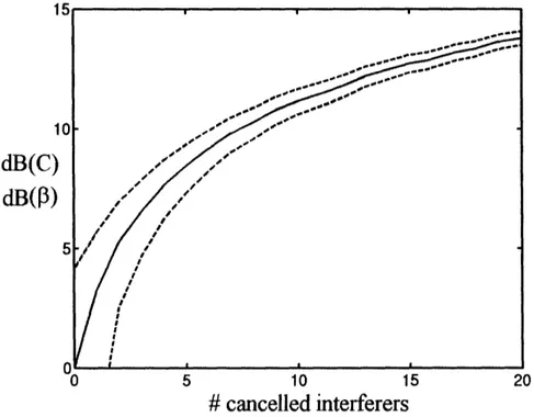
The practical definition of capacity (with fixed bit error rate and Eb = 5dB) is

No

proportional to SINR and P (see (20)), and as a consequence, the dB improvement of this

capacity is the same as the dB improvement of f. The results for both/ and capacity

defined in (20) is given in Figure 5.

dB(C

dB(P

D

# cancelled interferers

Figure 5: Improvement in dB of P and link capacity as defined in (20), plotted against the number of

interferers subtracted in the SIC strategy. The solid line is the average result, and the dashed lines

correspond to the average plus or minus the standard deviation of results.

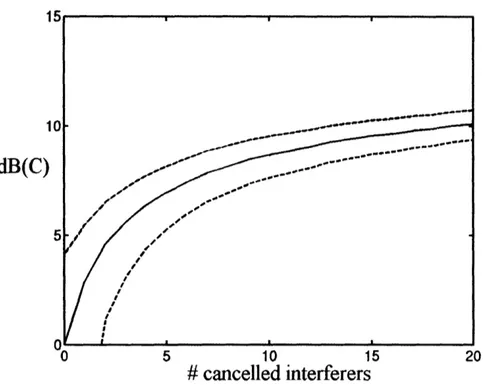
The other definition of capacity, which was derived from the Shannon' s limit and

described in (19), is proportional to the logarithm of an expression containing P. That is why the dB improvement of such capacity depends on the original capacity value. In our case, since the capacity in (19) depends on the rank R of the link, it means that the dB improvement of capacity also depends on the rank of the link. That is why the results are

1

dB(C)

0 5 10 15

# cancelled interferers

20

Figure 6: Improvement in dB of link capacity as defined in (19), plotted against the number of interferers

subtracted in the SIC strategy. The result corresponds to the case when rank of the link R=2. The solid line is the average result, and the dashed lines correspond to the average plus or minus the standard deviation of results.

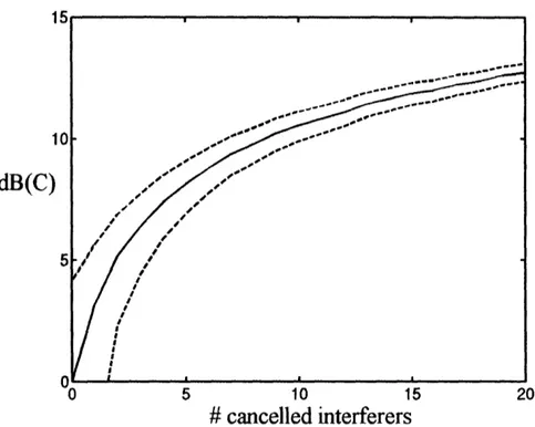
dB(C'

# cancelled interferers

Figure 7: Improvement in dB of link capacity as defined in (19), plotted against the number of interferers

subtracted in the SIC strategy. The result corresponds to the case when rank of the link R=3. The solid line is the average result, and the dashed lines correspond to the average plus or minus the standard deviation of results.

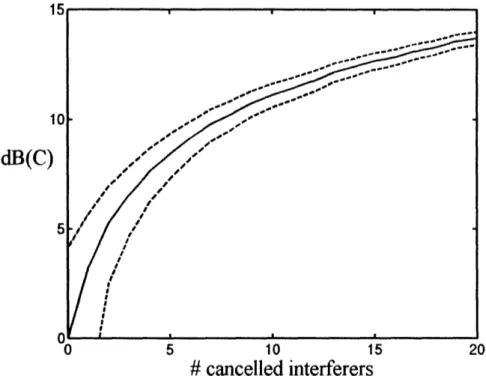
4 r

!

1

1

dB(C)

l

# cancelled interferers

Figure 8: Improvement in dB of link capacity as defined in (19), plotted against the number of interferers

subtracted in the SIC strategy. The result corresponds to the case when rank of the link R=5. The solid line is the average result, and the dashed lines correspond to the average plus or minus the standard deviation of results.

dB(C

)

# cancelled interferers

Figure 9: Improvement in dB of link capacity as defined in (19), plotted against the number of interferers

subtracted in the SIC strategy. The result corresponds to the case when rank of the link R=10. The solid line is the average result, and the dashed lines correspond to the average plus or minus the standard deviation of

1

1

dB(C)

# cancelled interferers

Figure 10: Improvement in dB of link capacity as defined in (19), plotted against the number of interferers

subtracted in the SIC strategy. The result corresponds to the case when rank of the link R=20. The solid line is the average result, and the dashed lines correspond to the average plus or minus the standard deviation of

results.

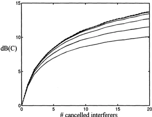
All these results are combined in the same plot in Figure 11, where one can see

how the improvement curves shift upwards when R changes. The solid curves on the

graph are all below the dashed line, and they correspond to the Shannon capacity from

formula (19). The lowest of them is the result for R = 2, and as R increases, the

improvement curves shift upwards. The dashed curve corresponds to the capacity defined

by (20), and we can see that the solid curve for R = 20 lies almost at the same level as the dashed curve. That tells us that for high values of R the capacity improvement curves are the same for the two capacity definitions.

One can see that the greatest discrepancy of the improvements for two different capacities exists for R = 2 (see Figure 11), where the difference between the two curves is around 3.5dB for 20 subtracted interferers. This means that the gap between the Shannon limit and the achievable capacity (from formula (20)) decreases. The original gap, as noted in chapter 3, was around 6.2dB for R = 2, and for 20 subtracted interferers we can see that this gap can be reduced to less than half of its original value if you

eliminate 20 closest interferers.

1

1

dB(C)

D

# cancelled interferers

Figure 11: Improvement in dB of link capacity vs. number of interferers subtracted in the SIC strategy.

The solid curves correspond the Shannon's capacity defined in (19), and they are plotted for the rank values, from bottom to top: R=2, 3, 5, 10, 20. The dashed curve on top corresponds to the improvement of the capacity defined in (20).

These plots achieve the goal of this chapter to present what happens with the link capacity when one uses the SIC strategy for enhancing the performance of the system. The plots of capacity improvement can be compared to the plots achieved with the multiple antenna system that is described in the following chapter, and the tradeoffs between the two strategies then become clear.

Chapter 4:

Multiple Antennas

4.1. Motivation

The link capacity that we looked at until now was derived for single antennas at each user, with equal antenna gain in all directions. This is not very practical since that way the receivers suffer interference coming from all directions, and the transmitters waste their power by transmitting with equal intensity in all directions instead of concentrating on the direction where the target receiver is located. As a consequence, a suboptimal SINR is achieved at the receiver's end of the link, and link capacity, which

depends on the SINR, also stays at levels that are lower than in the case of appropriately designed non-isotropic antennas. The goal of this chapter is to examine what is the

difference in the performance of the system when appropriately designed non-isotropic

antennas are used.

In order to enhance the performance of the system, one should use directional

antennas, with the lobes of the antenna gain pattern pointing towards the corresponding receiver or transmitter. There are many types of directional antennas, as described in [22], but in this thesis I use multiantenna arrays, which in effect can have a gain pattern same as directional antennas, just as long as correct multipliers are applied to each individual antenna in the antenna array. The difference between a directional antenna and a multiantenna array used in this thesis is in the fact that arrays consist of multiple individual isotropic dipole antennas. These isotropic dipole antennas are then multiplied by a complex vector, which corresponds to amplitude and phase shifts, and the sum of the multiplied signals is equal to the input signal in the multiantenna system. This way one can create a wide variety of antenna gain patterns, with lobes and nulls in optional directions. One is only limited by the number of peaks and nulls that can be placed in desired directions, since the number of degrees of freedom is limited by the number of dipole antennas in the array.

The reason for studying the effects of multiantenna arrays in this thesis lies in

possible practical implementations of the system. Isotropic dipole antennas are simple to

build and connect together. Also, after the array is built, one does not have to physically rotate the array in order to position a lobe in the desired direction, or place a null on an

interferer, but instead, one just needs to find the optimal complex vector of multipliers,

while the array stays physically in the same place. That would not be the case with some basic types of directional antennas, which is an advantage of multiantenna arrays over

such directional antennas.

The array of isotropic antennas can, further, be attached to edges of a device, such as a laptop computer, which is a very likely candidate for a typical user in the wireless network we are trying to design. Later in the chapter I discuss what is the minimum spacing between the antennas in the antenna array, and the result that I got was iA, where 2 is the wavelength of transmitted signal. The bands that are likely to be reserved

for wireless ad hoc networks are probably either going to be around 2GHz or 5GHz. For

these frequencies, the corresponding wavelengths are equal to:

3-

m/s

2. 109Hz

3 10 mls

and

2=

/s= 0.06m.

(22)

5.10

Hz

From here we see that the minimum distances are 7.5cm and 3cm, which means that the dipole antennas of the array can be attached to edges of a laptop, or an even smaller device. In conclusion, multiantenna arrays are likely to be easily implemented in wireless ad hoc networks. In this thesis, I concentrate on the performance of multiple antennas in simulation-oriented experiments under specific conditions.

4.2. Assumptions

Most of the conditions under which the formulas (19) and (20) were derived are valid in this chapter as well. All receivers and transmitters are randomly and uniformly

distributed in a plane with equal density

u

_{and paired up in data communication}

links consisting of one receiver and one transmitter. All transmitters that are not in the link are considered to be interferers at the receiver of that link, and thermal noise of the receiver is considered to be negligible compared to the interference level at the receiver.

The difference from chapter 2 is in the fact that instead of one dipole isotropic antenna, users now have n isotropic dipole antennas arranged in an array (n Ž 2). All n

antennas of a user are positioned in the plane of the network, vertically oriented,

perpendicular to the plane and with isotropic individual gains in the plane. However, these antennas in combination have a non-isotropic gain pattern, with lobes and nulls in

different directions, which depend on the complex multiplier vector with which the

individual antenna signals are multiplied (vector

from equation (25)).

Transmitting and receiving users can both have multiantenna arrays, but in this

thesis they have slightly different strategies. While a transmitter only tries to put

maximum gain on the corresponding receiver, a receiver tries to both put a high gain on the corresponding transmitter and null its strongest interferers. It is important to notice

that the communication approach in this chapter is not strictly speaking MIMO, although

this kind of communication could be considered MIMO, since both transmitters and

receivers have multiple antennas. Instead of looking at communication between multiple

transmitting antennas and multiple receiving antennas all at once (MIMO approach), this chapter examines what happens separately at the receiving and transmitting end of the

link, and distinguishes the contributions of the two to the link capacity.

Receivers

The receiving end of the link receives signals from many transmitters in its surroundings that act as interferers, as well as the desired transmitter from the other end of the link. The signal coming from a transmitter to the n receiving antennas is

represented by a vector , whose entries are the received signals at individual antennas:

= v s,

(23)