Scheduling inspection and renewal of large infrastructure assets

Publisher’s version / Version de l'éditeur:

Journal of Infrastructure Systems, 7, December 4, pp. 136-143, 2001-12-01

READ THESE TERMS AND CONDITIONS CAREFULLY BEFORE USING THIS WEBSITE. https://nrc-publications.canada.ca/eng/copyright

Vous avez des questions? Nous pouvons vous aider. Pour communiquer directement avec un auteur, consultez la

première page de la revue dans laquelle son article a été publié afin de trouver ses coordonnées. Si vous n’arrivez pas à les repérer, communiquez avec nous à PublicationsArchive-ArchivesPublications@nrc-cnrc.gc.ca.

Questions? Contact the NRC Publications Archive team at

PublicationsArchive-ArchivesPublications@nrc-cnrc.gc.ca. If you wish to email the authors directly, please see the first page of the publication for their contact information.

NRC Publications Archive

Archives des publications du CNRC

This publication could be one of several versions: author’s original, accepted manuscript or the publisher’s version. / La version de cette publication peut être l’une des suivantes : la version prépublication de l’auteur, la version acceptée du manuscrit ou la version de l’éditeur.

For the publisher’s version, please access the DOI link below./ Pour consulter la version de l’éditeur, utilisez le lien DOI ci-dessous.

https://doi.org/10.1061/(ASCE)1076-0342(2001)7:4(136)

Access and use of this website and the material on it are subject to the Terms and Conditions set forth at Scheduling inspection and renewal of large infrastructure assets

Kleiner, Y.

https://publications-cnrc.canada.ca/fra/droits

L’accès à ce site Web et l’utilisation de son contenu sont assujettis aux conditions présentées dans le site LISEZ CES CONDITIONS ATTENTIVEMENT AVANT D’UTILISER CE SITE WEB.

NRC Publications Record / Notice d'Archives des publications de CNRC:

https://nrc-publications.canada.ca/eng/view/object/?id=930af743-370a-436c-bc75-a56072bd471a https://publications-cnrc.canada.ca/fra/voir/objet/?id=930af743-370a-436c-bc75-a56072bd471a

Scheduling inspection and renewal of large infrastructure assets

Kleiner, Y.

A version of this paper is published in / Une version de ce document se trouve dans:

Journal of Infrastructure Systems, v. 7, no. 4, Dec. 2001, pp. 136-143

www.nrc.ca/irc/ircpubs

Scheduling Inspection and Renewal of Large Infrastructure Assets

Abstract

A decision framework is introduced to assist municipal engineers and planners to optimise decisions regarding the renewal of large infrastructure assets, such as water transmission pipes, trunk sewers or other assets with high costs of failure, inspection and condition assessment. The proposed decision framework identifies a need for immediate intervention or alternatively, enables to optimise the scheduling of the next inspection and condition assessment.

The deterioration of the asset is modelled as a semi-Markov process, thereby discretised into condition states. The waiting times in each state are assumed to be random variables with ‘known’ probability distributions. If pertinent data are scarce (as is typical in most

municipalities) these probability distributions can be initially derived based on expert opinion. These distributions will then be continually updated as observed deterioration data are collected over time. Monte-Carlo simulation is used to calculate the distributions of the cumulative waiting times. Conditional survival probabilities are used to compile

age-dependent transition probability matrices in the various states. The expected discounted total cost associated with an asset (including cost of intervention, inspection and failure) is

computed as a function of time. The time to schedule the next inspection/condition

assessment is when the total expected discounted cost is minimum. Immediate intervention should be planned if the time of minimum cost is less than a threshold period (2 to 3 years) away.

A computer program was prepared for demonstration and proof of concept. The decision framework lends itself to a computer application fairly easily. Although usable in its current form, this paper identifies some issues that require as yet unavailable data as well as more research in order to develop the framework into a comprehensive application tool.

Key words: Buried utilities renewal, scheduling inspection/condition assessment, scheduling intervention, semi-Markovian deterioration.

Introduction

Large infrastructure assets typically have low failure rates but when they fail the

consequences can be severe. This low rate of failure, coupled with high cost of inspection and condition assessment, seems to have contributed to the current situation where most municipalities lack the data necessary to model the deterioration rates of these assets and subsequently make rational decisions regarding their renewal.

The decision tools that are currently prevalent in this area are largely in the form of

guidelines where distress indicators observed in the asset are translated into asset condition states and recommendations are prescribed as to the required course of action at each condition state. The recommendations depend on the severity of the relevant condition state and on the perceived impact of failure. Examples of such guidelines include WRc (1993, 1994), Edmonton (1996) and Zhao and McDonald (2000) among others. These guidelines are extremely useful for the mapping of distress indicators into condition states. This mapping is an essential component of any decision tool. However, the decision process that these guidelines provide are largely qualitative and prescriptive (e.g., “condition state x requires that the asset be inspected every y years”), and as such tend to be rather broad and general. Further, economics and deterioration rates are considered only in an implicit and fuzzy manner.

The literature reflects various efforts to provide quantitative-based decisions to infrastructure or other components of the built environment. The Factor Method was developed by The International Organisation for Standards (ISO) to estimate service life of built components (ISO/CD 16696-1, 1997). The method simply multiplies the reference service life of the component by factors affecting it (e.g., the factor for high level of maintenance may be greater than 1 – acting to extend the life of the component, whereas harsh outdoor environment may add a factor smaller than 1 – acting to shorten its life). The values of these factors can be determined by a Delphi process (Moser, 1999) or individual experience. Aarseth and Hovde (1999) showed how the Factor Method could be applied in a probabilistic manner. The Factor Method may not be suitable to buried infrastructure

because of insufficient data to determine reference service life. Flourentzou et al. (1999) developed an approach in which the life of every built element is divided into four condition

states, good, fair, poor and need replacement. With sufficient field data, the age distribution of a component in any condition state can be estimated. Using conditional probabilities, the time to replacement and the expected cost can be estimated. Abraham and

Wirahadikusumah (1999) modelled the deterioration of sanitary sewers as a Markov chain process. They divided the life of the asset into four phases, whereby the deterioration in each phase is characterised by a stationary transition matrix. These transition matrices are compiled using expert opinion. Kathula and Mckim (1999) used markov-chain process to model sewer deterioration. They compiled (homogeneous) transition probabilities based on a survey of 55 sewer management experts, who responded to a detailed questionnaire about their own sewer system. Ariaratnam et al. (1999) reported good results using a multinomial logit model to model the likelihood of a sewer being in a deficient state given age category, material type, effluent transported, diameter category and depth category. The sewers then were ranked in an ascending order of likelihood, to provide a priority list for inspection. In this paper an approach is presented to make the decision process more quantitative and explicit and specific to the asset at hand and its unique set of circumstances. The

deterioration of the asset is modelled as a semi-Markov process, which means that the condition of the asset is discretised into a finite number of states. The durations of the asset in each condition state, also called state waiting times, are modelled as random variables with known probability distributions. These probability distributions are used to derive the transition probabilities from one state to the next. The transition probabilities are inherently age-dependent, which means that the older the asset, the higher the likelihood of

deterioration to the next state in a given period of time. The total expected cost associated with the asset can then be calculated as a function of time, and a decision made as to whether to rehabilitate or schedule the next inspection/condition assessment.

Currently there are insufficient historical data to populate the deterioration models and to derive their parameters. Consequently it is envisaged that the approach could be applied in two phases. In the short term, for lack of field data, parameters for the waiting times

probability distributions can be derived based on expert opinions. These expert opinions are also the basis for the qualitative methods used in the current state of the practice. However, the proposed approach puts numbers to these opinions and then forces a decision that is a

direct, rational and precise outcome of the expert opinion. In the long term the parameters will be continually updated using actual survival data collected from the field.

The rest of this paper is organised as follows. The next section describes the modelling of the deterioration in buried assets, including theoretical fundamentals of Markov and semi-Markov processes and how they are implemented in the proposed method. The two subsequent sections describe the costs that are associated with asset life-cycle and the decision process. Summary and conclusions are provided in the last section including an identification of issues that require further research.

Buried asset deterioration model

Fundamentals of Markov and semi-Markov processes

Parzen (1962) defined a discrete time Markov process as a stochastic process with

parameters X(t), that for any n time points t1, t2,…tn the conditional distribution of X(tn),for given values of {X(t1),…, X(tn-1)} depends only on X(tn-1), which is the most recent known value. This can be stated as

[1] Pr

[

] [

]

This equation can be interpreted to mean that the future of the process depends only on the present and not on the past. Parameters {X(tk);k=0,1,2,…} are random variables representing the state of the process at time points, tk. The values {xi, i=1,2,...,n} comprise the state space of the process. A Markov process with a discrete state space is called a Markov chain. When the Markov process goes from state xi to state xj, it is said that a transition has occurred. For simplicity we can call it transition from state i to state j. A Markov chain is determined by a transition probability function, which is the conditional probability of a transition from state i to state j during a given period of time. A single step transition probability p_ijt,t+1 from state i to state j is defined:

[2] p_ijt,t+1 =Pr

[

]

[3] p_ijt,t+1 = p_ij0,1 = p_ij

it is said that the Markov chain is stationary in time (or homogeneous). A Markov transition probability matrix Pt,t+1

(

ij t,t+1

; i,j = 1,2,..n

)

[4] ; 0 (, 1,2,.., ); 1 ( 1,2,.., ) ... ... ... ... ... ... ... ... 1 1 1 1 1 1 1 2 1 22 1 21 1 1 1 12 1 11 1 , , , , , , , , , , , n i p n j i p p p p p p p p p P n j ij ij nn n n n t t t t t t t t t t t t t t t t t t t t t t _{≥ = ∑ = =}               = = + + + + + + + + + + +

In an n-state space discrete Markov process, the state of the process at any time t is typically stochastic and is defined by a probability mass function (pmf) that is denoted by an

n-dimensional vector A(t).

[5] = ∑ = = n i i n t t t t a a a a t A 1 2 1, ,... } ; 1 { ) (

Member ait denotes the probability that the process is in state i at time t. The probability mass function of the process at time (t+1) is obtained

[6] ( 1) ( ) { , ,... } ; ,( 1,2,... ) 1 1 1 1 1 2 1 1 1 , , _{a a a a a p i n} P t A t A n j j ji i n t t t t t t t t t _{= = ∑ =} = + = + + + + + +

The probability mass function of the process at time (t+k) is obtained [7] A(t+k)= A(t)Pt,t+1Pt+1,t+2...Pt+k−1,t+k

For a stationary Markov chain equation (7) can be reduced to [8] _A(t+_k)= _A(t)Pk

A Markovian process with sojourn (or waiting) times in any given state that are

independently distributed random variables, is referred to as a semi-Markov process. The conditional sojourn time in state i, given that the process goes to the next state j is denoted by Tij, and has a probability density function (pdf) denoted by fij(t), a cumulative density function (cdf) denoted by Fij(t) and a survival function (sf) denoted by Sij(t).

Modelling deterioration using semi-Markov process

In the proposed decision framework the semi-Markov process is used to model

deterioration. It is assumed that if no intervention (renewal or rehabilitation) is implemented the process is unidirectional, i.e., if state 1 denotes good as new and state n denotes failure, then the process can move only from state i to state j where j = i. Further, it is often assumed (e.g., Madanat et al., 1995) that an infrastructure asset can deteriorate only one state at a time, that is, the asset will deteriorate from state 1 to state 2, then to state 3, and so on to failure (providing no renewal was implemented). The process thus cannot jump from state 1 to state 3 without passing through state 2. (Kathula and Mckim, 1999 reported sewers, which had deteriorated more than one state in a single stage, however, their process comprised uniform transition periods of five year each. If an asset is expected to deteriorate very fast one can shorten transition periods to the extent that realistically only single state deterioration is possible in one period). This results in a relatively simple transition probability matrix [9]                 = + + − + − − + + + + + 1 1 , 1 1 1 , 1 1 23 1 22 1 12 1 11 1 , , , , , , , , 0 .... 0 0 .... .... 0 .... .... .... .... .... 0 ... 0 0 ... 0 t t t t t t t t t t t t t t t t nn n n n n p p p p p p p P

Under the assumptions stated above, it is now possible to simplify some of the notation used so far. We shall denote the following:

T1, T2,…, Tn-1 are random variables denoting the sojourn times in states {1, 2,…, n-1}, respectively (rather than Tij because the index j is always equal to i+1, therefore it can be dropped). Their corresponding pdfs, cdfs and sfs are thus denoted fi(t), Fi(t), Si(t).

TiÕk is a random variable denoting the sum of sojourn times in states {i, i+1,…, k-1} This can be expressed as T k 1T_{, 1} ; i {1,2,...,n 1}, k {2,3,...,n} i j j j k i = ∑ = − = − = + → . Thus, Ti_Õk is the

time it will take the process to go from state i to state k. In addition, fi_Õk(Ti_Õk), Fi_Õk(Ti_Õk),

If the deterioration process is in state 1 at time t, the conditional probability that it will transit to the next state in the next time step ∆t is given by

[10] ) ( ) ( ) ( ] 1 ) ( 2 ) 1 ( Pr[ 1 1 2 , 1 t S t t f t p t X t X + = = = = ∆

where t = 0 is the time when the process entered into state 1 (i.e., new asset – in most cases). The formulation in equation (10) corresponds to discrete time steps that are assumed small enough to exclude a two-state deterioration. In subsequent formulations ∆t is assumed to be one unit (year) and is thus omitted.

If the process is in state 2 at time t, the conditional probability that it will transit to the next state in the next time step ∆t is given by

[11] ) ( ) ( ) ( ) ( ] 2 ) ( 3 ) 1 ( Pr[ 1 2 1 2 1 3 , 2 t S t S t f t p t X t X − = = = = + → →

where t = 0 is the time when the process entered into state 1. Note that in equation (11) the pdf in the rhs numerator pertains to T1Õ2, whichis the random variable denoting the sum of sojourn times in states 1 and 2. Further, the denominator expresses the simultaneous

condition that T1Õ2 < t and T1 < t, which is equivalent to the condition X(t) = 2. Equation (11) can be generalised by [12] ; {1,2,..., 1} ) ( ) ( ) ( ) ( ] ) ( 1 ) 1 ( Pr[ ) 1 ( 1 1 1 1 , = − − = = = + = + − → → → + i n t S t S t f t p i t X i t X i i i i i

The conditional probability in equation (12) provides all the transition probabilities pi,i+1(t) to populate the transition probability matrix for the semi-Markov process. These transition probabilities are time-dependent, i.e., the process is assumed to be stationary (or non-homogeneous). This property of non-stationary deterioration of infrastructure assets has been observed by others, e.g., Jiang et al. (1989), Madanat et al. (1995, 1997), Guignier (1999).

Once the transition probability matrix is established, the deterioration process can be modelled by using equation (7) to obtain the probability mass function (pmf) of the process at any time t. If state n is defined as failure (see definition of failure in the Section

“Consideration of costs”) and if at time t the asset has a pmf A(t)={a1, a2,…, an} (equation 5), that means that the probability that the asset will fail at time t is an.

If the asset is assumed to be good as new (entering state 1) at age zero, then the pmf of the process becomes, in effect, age-dependent. Note that age zero need not necessarily be a chronological age, it is rather a functional age at which the process is entering state 1 and is as good as new. Thus, it can happen that a newly installed asset has some defects and is not entirely in state 1 although its chronological age is zero. Conversely, an asset can

functionally be at age zero after undergoing major rehabilitation.

Modelling waiting times in the semi-Markov process

We shall arbitrarily assume that the waiting time Ti of the process in any state i can be modelled as a random variable with a two-parameter Weibull probability distribution.

[13] i i i i i i i i i i i i i i i i t t t e t t t F t f e t F t S e t T t F β β β λ β λ λ λ β λ ( ) ) ( ) ( 1 ) ( ) ( ) ( ) ( 1 ) ( 1 ] Pr[ ) ( − − − − = ∂ ∂ = = − = − = ≤ =

It should be noted that the procedure is not limited to any one distribution, and that it is even possible to use different distributions for different states in the same deterioration process. The pdf, cdf and sf, fiÕk(TiÕk), FiÕk(TiÕk), SiÕk(TiÕk) of the sum of waiting times

} ,..., 2 , 1 { }, 1 ,..., 2 , 1 { ; 1 1 , i n k n T T k i j j j k i = ∑ = − = − = +

→ cannot generally be calculated

analytically, therefore Monte-Carlo simulations can be used to numerically calculate these functions for sums of Weibull-distributed random variables Ti_Õk.

Deriving parameters for the deterioration model

There are currently insufficient data to derive parameters ?i and ßibased on historical observations and condition assessments of large buried assets. Consequently, these parameters will initially have to be derived from expert opinion and perception. The following process is suggested. An expert or a group of experts (e.g., in a Delphi process) would have to answer questions pertaining to their beliefs about the likelihood of an asset remaining in a given state for a certain period of time. For example, the following statement

would have to be made: “In my opinion, the asset has a probability of xi,u of being in state i more than u years”. Since there are two parameters ?i and ßito be estimated for every state i, two such statements have to be made for every state i, i={1, 2,…, n-1}, with u years and v years, u ? v, to produce two quantiles xi,u and xi,v. Parameters ?i and ßi are then derived in the following manner: [14]

(

) (

)

₍

₎

Once parameters ?i and ßi are established for every i = {1,2,…, n-1}, the transition probability matrix can be calculated by substituting equation (13) into equation (12).

Illustrative example case

For lack of historical data on deterioration rates, all the examples provided in this paper are hypothetical. Suppose the state space of a large buried asset comprises 5 states, where state 1 is good as new and state 5 is failure (see definition of failure in the Section “Consideration of costs”). Suppose further that a group of experts have determined that, for this type of asset under similar conditions, if the asset is as good as new at age zero then the probabilities in Table 1 apply, with parameters ?i and ßi derived using equations (14).

Table 1. Example case: expert opinions tabulated as probabilities of survival. State i u (years) xi,u v (years) xi,v ßi ?i

1 15 50% 25 10% 2.350 0.057

2 25 50% 35 10% 3.568 0.036

3 10 50% 20 10% 1.732 0.081

4 10 50% 15 10% 2.961 0.088

Note: The asset is xi,u% likely to remain in the state i more than u years, and xi,v% likely to remain in the state i more than v years:

Next, parameters ?i and ßi and equations (13) are used to produce pdf, fi(t), cdf, Fi(t), and sf,

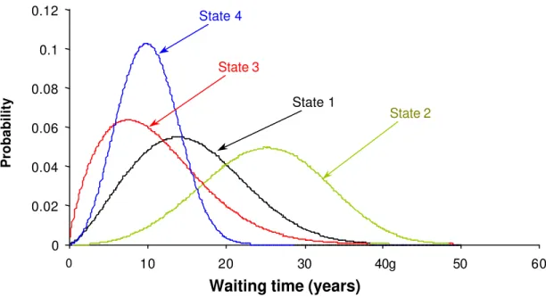
states vary significantly. For instance, the mean waiting time in state 2 is about 25 years but the dispersion is relatively large and the time can vary from less than 10 years to more than 40 years. Conversely, the mean waiting time in state 4 is about 10 years with a much smaller variation.

Figure 1. Exampl: pdfs of waiting times in all condition states.

The next step is to find the sums of waiting times in the various states, TiÕk, and their respective pdfs, cdfs and sfs. These values are obtained numerically using Monte-Carlo simulations to generate (n - 1) Weibull-distributed random numbers with parameters ?i and

ßi. Figures 2 and 3 illustrate the resulting pdfs and sfs.

It can be seen that, in this example, the mean time to failure is about 60 years. Recall that state 5 was defined as failure, thus the pdf of states 1+2+3+4 defines the pdf of asset age at failure, given that it is as good as new at age zero. Further, it can be seen that the vast majority of buried assets of this type under similar sets of conditions are expected to last between 40 and 90 years.

Figure 3 demonstrates the survival function of the process and how it changes over the life of the asset, given that it was good as new at age zero. In this example, the asset at age 28 is about 4% likely to still be in condition state 1, about 78% likely to be in state 2, about 16%

0 0.02 0.04 0.06 0.08 0.1 0.12 0 10 20 30 40g 50 60 Age (years) Probability State 3 State 1 State 2 State 4

likely to be in condition state 3, and about 2% likely to be in state 4. The probability of failure at age 28 is virtually zero.

Figure 2. Example: pdfs of cumulative waiting times in various states.

Figure 3. Example: Survival functions of cumulative waiting times in various states.

0.00 0.01 0.02 0.03 0.04 0.05 0.06 0 20 40 60 80 100 Age Probability State 1 States 1+2 States 1+2+3 States 1+2+3+4

Cumulative waiting time (years)

0 0.2 0.4 0.6 0.8 1 0 20 40 60 80 100 Age (years) Probability

1

2

3

4

5

The next step is to generate the age-dependent transition probabilities pi,i+1(t), using equation (12). Once these transition probabilities are determined, the deterioration process of any buried asset can be modelled without knowing whether it was as good as new at age zero.

Suppose a large, 20-year old asset is to be analysed. An inspection and condition assessment have determined that there is some uncertainty about the precise state of the asset, thus it is in state 1 with a probability of 60%, in state 2 with a probability of 30%, and in state 3 with 10% probability. From equation (5) we obtain the asset pmf at age 20 years,

[15] A(t)={a1,a2,...a}=A(20) ={0.6,0.3,0.1,0,0}

t t t

n

where t denotes the asset age.

By applying equation (12) as described above the transition probability matrix for a 20-year old asset can be found,

[16]               = 1 0 0 0 0 006 . 0 994 . 0 0 0 0 0 019 . 0 981 . 0 0 0 0 0 005 . 0 995 . 0 0 0 0 0 160 . 0 840 . 0 21 , 20 P

It can be seen that if an asset is in state 1 at age 20, during the next year it is 84% likely to remain in state 1 and 16% likely to deteriorate to state 2, etc. Equation (6) can then be used to obtain the pmf of the asset at age 21,

[17] } 0 , 002 . 0 , 100 . 0 , 395 . 0 , 504 . 0 { } 0 , 0 , 1 . 0 , 3 . 0 , 6 . 0 { 1 0 0 0 0 006 . 0 994 . 0 0 0 0 0 019 . 0 981 . 0 0 0 0 0 005 . 0 995 . 0 0 0 0 0 160 . 0 840 . 0 1 , ) ( ) 1 ( =               = = = + tt+ P t A t A

In general, if the analysis is done at year

τ

τ

[18] = ∏− = + + + 1 0 1 , 0 0 0 ) ( ) (τ τ k ij k kt t P t A A

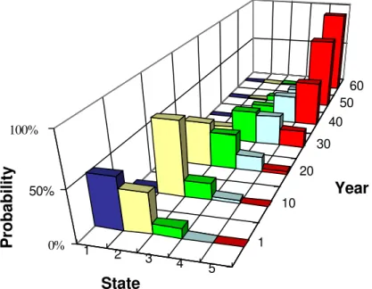
Figure 4 illustrate how the pmf of our example assets varies over time from the present to the future.

Figure 4. Example: Progression of asset pmf over time.

Consideration of costs

In the following sections, per unit costs of products and services are assumed to be in constant dollars quoted at the time of analysis. Discount rate is assumed to be the effctive rate, net of inflation.

Failure cost. Failure is defined as an event where an unplanned emergency intervention is required to restore or to prevent imminent loss of operability. The cost of failure CF includes emergency repair, direct damages, indirect costs and social costs. While indirect and social costs are hard to quantify, an effort should be made to provide a rational

approximation. The expected cost of failure at age t is the product of the cost of failure and the probability of failure at age t, i.e., E[CF(t)]=CF atn.

Inspection and condition assessment cost. These may vary with the type, size, depth, accessibility and functional state of the asset. This cost is denote by CI and is assumed to be time-independent. 1 ₂ 3 ₄ 5 1 10 20 30 40 50 60 0% 50% 100% State Year Probability

Planned intervention cost. The cost of planned intervention (rehabilitation, renovation) depends on many factors. It is generally assumed that intervention with an asset in state i may have a different cost than intervention with the same asset in state j, i ? j. Thus, the

expected cost of intervention at age t is t T

n t t r n r r R a a a c c c t C E[ ( )]={ 1, 2,..., −1}⋅{ 1, 2,..., −1} , where cri is the cost of planned intervention with an asset in state i.

The decision horizon of buried assets may encompass many years, therefore the time-value of money has to be considered by time-discounting all future cash flows. The total

discounted expected cost that is associated with the asset at time τ is expressed with the continuous form of discounting

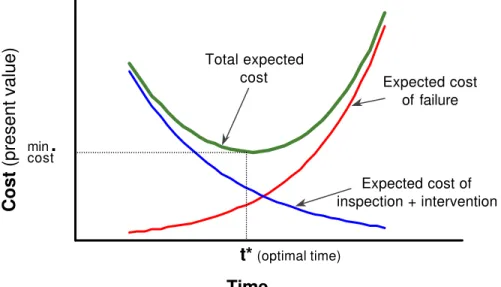
[19] Ctot(τ)=

(

)

where r is the discount rate and t0 is the age of the asset at the present time, when τ = 0. The expected cost of failure increases with time due to the increase in the probability of failure. Discounting reduces the rate of this increase, however, typically there will be a time period in which the probability of failure increases faster than the discounting effect,

resulting in an increasing failure cost. The expected cost of intervention typically increases over time because it is usually more expensive to intervene at a higher state of deterioration. However, the effect of discounting is typically stronger, resulting in a decreasing cost curve. Since the cost of inspection/condition assessment is assumed to be time-independent, the discounted cost of inspection/condition assessment is always decreasing over time. These effects typically result in a convex total cost curve as illustrated in Figure 5.

The decision process

The decision process comprises the following fundamental assumptions:

• An optimal decision strategy would minimise the total expected costs that are associated with the buried asset throughout its life.

• Upon inspection and condition assessment, the decision alternatives are: 1. no immediate intervention is required, therefore the next

inspection/condition assessment must be scheduled, or, 2. an immediate intervention is required.

Note that “immediate” in this context can mean a threshold period of one to three years. In the realm of large buried infrastructure assets, planning, designing bidding and executing rehabilitation projects require this threshold period.

• A decision is always preceded by an inspection/condition assessment. It is unlikely that an intervention will be planned more than two to three years (the threshold period) in advance.

Ideally, intervention should be implemented just before failure, thus benefiting from the deepest possible discount on the cost of intervention, while avoiding high failure costs. In reality the probability of failure can only be evaluated at any given time, thus the objective is to defer intervention as much as possible without taking too high a risk of failure. This objective can be achieved by continuously evaluating the marginal benefits of postponing intervention by one additional year against the marginal increase in failure risk of an asset, which is one year older.

Figure 5. Expected costs variation over the asset life-time.

The benefits of deferral are expressed in terms of discounted expected costs of intervention and inspection {E[CR(t0+τ)]+CI}e-rτ. The failure risk is expressed in terms of discounted expected cost of failure E[CF(t0+τ)]e-rτ. Assuming that the sum of these expected costs forms a convex curve over time (Figure 5), the point of minimum total expected cost,

t* = t0 + τ∗ denotes the age at which the marginal benefit of deferral equals the marginal

τ Total expected cost min

.

However, one of the fundamental assumptions made was that any intervention must be preceded by an inspection/condition assessment, which implies that the asset must be inspected at time τ* before commencing rehabilitation. After assessing the condition of the asset at time τ*, its true probability mass function (pmf) can be evaluated and compared to the predicted pmf. If the true pmf is approximately “equal to” or “worse than” the predicted pmf, then indeed τ* is the optimal time for intervention. If, on the other hand, the true pmf is “better (less deteriorated) than” the predicted pmf, then it is too early to intervene; the

deterioration model should be re-applied with the new pmf in order to find a later optimal time τ**.

The terms ‘equal’, ‘better’ and ‘worse’ above are enclosed in double quotations because the pmfs (probability mass functions) are vectors and it may be difficult to determine which vector is “better” or “worse”. For instance, if at time τ* the predicted pmf is

{0, 0, 0.2, 0.8, 0} and the observed pmf is {0, 0, 0.1, 0.9, 0}, then it is clear that the

observed is worse than the predicted. However, if the observed is {0, 0, 0.3, 0.6, 0.1}, then the comparison is ambiguous. In any case of ambiguity the asset should be re-evaluated with the observed pmf.

It should be noted that if the observed pmf is significantly better or worse than predicted, it may be necessary to update some or all the parameters ?i and ßi in light of the newly obtained data.

The decision process is illustrated using the example presented in the previous sections, where the pdfs and sfs of the cumulative waiting times in the various states are shown in Figures 2 and 3. The following costs are assumed:

Cost of failure, CF= $200,000

Cost of inspection and condition assessment, CI= $5,000

State _{1 2 3 4}

Cost of intervention at various states, CR =

Cost ($) 5,000 10,000 15,000 20,000

Discount rate, r = 4%

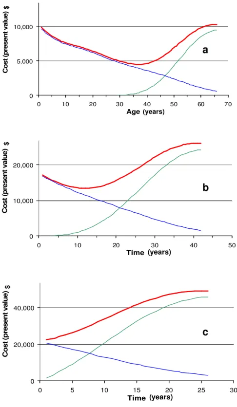
Suppose the asset is as good as new (entering state 1) at age zero. The discounted costs associated with it as a function of age (equation 19) are depicted in Figure 6a. The total

discounted costs associated with the asset appear to be minimum at t* = 37 years. That means that if post-installation inspection/condition assessment determine that the asset is in perfect condition, then the next inspection and condition assessment should be scheduled about 37 years after installation, based on expert opinion (as expressed in the parameter derivation procedure). The pmf of the asset at age 37 is predicted to be

A(37) = {0.002, 0.613, 0.298, 0.079, 0.008}.

Suppose that the asset was not inspected after installation, and that an inspection and

condition assessment implemented at age 20 determined that there was a 50% chance that it was in state 2, and 50% in state 3, i.e., its pmf observed was A(20) = {0, 0.5, 0.5, 0, 0}. Suppose further, that the expert opinions about this type of asset, under similar conditions have not changed following this last condition assessment. The analysis is then reapplied to the asset using equation (18), where A(t0) = A(20). Figure 6b illustrates the total costs obtained as a function of time τ. The total discounted costs associated with the asset appear to be minimum at τ* = 12 years. That means that the next inspection and condition

assessment should be scheduled after 12 years, i.e., when the asset is 32 years old.

Suppose that this scheduled inspection was carried out as planneded and that the condition assessment yielded a pmf of A(32) = {0, 0, 0.7, 0.3, 0}. Figure 6c illustrates the

corresponding cost curves. The total discounted costs associated with the asset appear to be minimum at τ** = 1 to 2 years. This means that intervention should be planned

immediately, since planning, tendering and implementing a scheduled intervention may require a threshold period of 1 to 3 years,.

Figure 6. Example: Total discounted expected cost in various scenarios. a. Cost as a function of age.

b. Cost as a function of time after age 20. c. Cost as a function of time after age 32.

0 5,000 10,000

0 10 20 30 40 50 60 70

Age

Cost (present value)

a

Cost (present value)

$

b

Cost (present value)

$

c

It is reasonable to assume that during the typically long intervals between inspections, new data obtained from other assets may lead to changes in expert opinions. For example,

suppose at the age of 20 years condition assessment determined that the pmf of the observed asset was better than expected, A(20) = {0.4, 0.6, 0, 0, 0}. Suppose further, that based on this observation and on observations on other similar assets, Table 1 was modified as in Table 2. It can be seen that the median and 90th percentile of the waiting times in states 1, 2, 3 have increased. The resulting cost curve is illustrated in Figure 7.

The total discounted costs associated with the asset appear to be minimum at τ* = 36 years, which means that the next inspection and condition assessment should be scheduled after 36 years, i.e., when the asset is 56 years old.

Table 2. Example expert opinions modified following new data.

State i u (years) xi,u v (years) xi,v ßi ?i

1 25 50% 35 10% 2.350 0.057

2 30 50% 40 10% 3.568 0.036

3 15 50% 20 10% 1.732 0.081

4 10 50% 15 10% 2.961 0.088

Figure 7. Example: Modified expected cost as a function of time after age 20.

0 5,000 10,000

0 10 20 30 40 50 60 70

Time

Cost (present value)

(years)

Summary and conclusions

A decision framework was described to assist municipal engineers and planners in

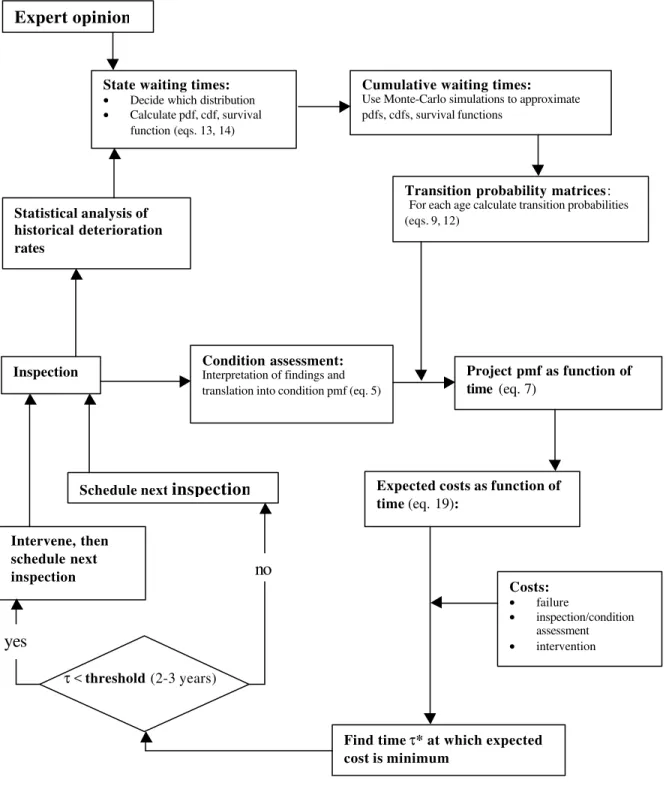
optimising the scheduling of rehabilitation as well as inspection and condition assessment of large buried assets, based on available data and expert opinion. Figure 8 provides a flow diagram for this decision framework. The key elements are:

• The deterioration of large buried assets is modelled as a semi-Markov process.

• The waiting times in each state are assumed to be random variables with known probability distributions. These probability distributions are initially derived based on expert opinion, and later are continuously updated as observed deterioration data are collected over time.

• The distributions of the cumulative waiting times in states 1+2, 1+2+3, and 1+2+3+4 are calculated using Monte-Carlo simulation.

• Age-dependent transition probability matrices are compiled, using conditional survival probabilities in the various states.

• The expected discounted total cost associated with an asset (including cost of intervention, inspection and failure) is computed as a function of time.

• The time to schedule the next inspection/condition assessment is when the total expected discounted cost is minimum.

• Immediate intervention should be planned if the time of minimum cost is less than a threshold period (2 to 3 years) away.

This framework was implemented in a computer program for proof of concept and demonstration. The framework is suitable for a computer application, however more research is required in the following areas, to develop a practical and comprehensive tool:

• As more deterioration data are collected over time, statistical procedures have to be developed for updating waiting time parameters. These procedures will be used to shift gradually from relying on expert opinion to using deterioration data. Since assets may deteriorate at different rates under various conditions, assets and data will have to be partitioned into groups comprising relatively homogeneous characteristics. Updating of the probability distribution parameters could be done using a statistical method such as

Bayesian updating (e.g., Ningyuan et al., 1997), however, More research is required to adopt this method to the process at hand.

Figure 8. Decision process flow diagram

Costs: • failure • inspection/condition assessment • intervention Project pmf as function of time (eq. 7)

Transition probability matrices:

For each age calculate transition probabilities (eqs. 9, 12)

State waiting times:

• Decide which distribution

• Calculate pdf, cdf, survival function (eqs. 13, 14)

Expert opinion

Condition assessment: Interpretation of findings and translation into condition pmf (eq. 5) Inspection

Cumulative waiting times: Use Monte-Carlo simulations to approximate pdfs, cdfs, survival functions

Find time τ* at which expected cost is minimum

Expected costs as function of time (eq. 19):

τ < threshold (2-3 years)

Statistical analysis of historical deterioration rates

Schedule next inspection

Intervene, then schedule next

inspection no

• The asset is assumed to begin a new deterioration mode after it has undergone

intervention (rehabilitation/renewal). This new deterioration mode may have a unique starting pmf as well as state waiting times. Different intervention alternatives can have different level of effectiveness at different costs. For example, alternative A can cost $10,000 to bring the deteriorated asset back to state 1, while alternative B costs $5,000 to bring the asset to state 2, or 3. Furthermore, these transitions to lower states are not deterministic but rather stochastic, with their own transition probabilities.

Data are required to determine transition probabilities from a deteriorated state to a renewed state, given various rehabilitation techniques (e.g., if an asset is in state 4 what is the probability that it would be in state 1 or 2 after it was lined with cement mortar). Further research is required to determined these transition probabilities and state waiting times, and to expand the decision framework to include the selection of the most

efficient rehabilitation/renewal alternative for a given buried asset in a given state.

• Economies of scale in buried assets rehabilitation costs can be an important factor. Their consideration in a decision optimisation procedure, however, is very challenging from a mathematical viewpoint. This issue warrants further research.

Acknowledgement

This research was part of the project Guidelines for Condition Assessment and

Rehabilitation of Large Sewers, managed by Jack Zhao of the Institute for Research in Construction (IRC), National Research Council of Canada (NRC). The project was sponsored by IRC and a consortium of municipalities and consultants including R.V. Anderson Associates Limited, M.E. Andrews & Associates Limited, Greater Vancouver Regional District, City of Calgary, City of Toronto, City of Edmonton, Regional

Municipality of Hamilton-Wentworth, Capital Regional District (Victoria), City of Waterloo, City of Regina, City of Saskatoon and the Region of Ottawa-Carleton.

References

Aaseth, L.I., and P.J. Hovde, (1999) “A stochastic approach to the factor method for estimating service life”, Proceedings of the 8th conference Durability of Building Materials and Components, Edited by M.A. Lacasse and D.J. Vanier, IRC, NRC, pp. 1247-1256, Vancouver.

Abraham, D.M., and R. Wirahadikusumah, (1999) “Development of prediction model for sewer deterioration”, Proceedings of the 8th conference Durability of Building Materials and Components, Edited by M.A. Lacasse and D.J. Vanier, IRC, NRC, pp. 1257-1267, Vancouver.

Ariaratnam, S.T., A. El-Assaly, and Y. Yang, (1999) “Sewer Infrastructure assessment using logit statistical models”, Proceedings, Annual Conference of the Canadian Society

for Civil Engineering, Regina, pp.330-338, June.

Edmonton City of, (1996) “Standard sewer condition rating system report”, City of

Edmonton Transportation Department, Canada.

Flourentzou, F., E. Brandt, and C. Wetzel, (1999) “MEDIC – a method for predicting residual service life and refurbishment investment budgets”, Proceedings of the 8th

conference Durability of Building Materials and Components, Edited by M.A. Lacasse and D.J. Vanier, IRC, NRC, pp. 1280-1288, Vancouver.

Guignier, F. and S. M. Madanat, (1999) “Optimisation of infrastructure systems

maintenance and improvement policies”, Journal of Infrastructure Systems, ASCE, Vol. 5, No. 4, Dec.

ISO/CD 16686-1, (1997) “Buildings: Service life planning, part 1 – general principles”,

ISO/TC59/SC3.

Jiang, Y., M. Saito, and K. C. Sinha, (1989) “Bridge performance prediction model using Markov chain”, Transp. Res. Rec. 1180, Transportation Research Board, Washington DC, pp 25-32.

Kathuls, V. S., and R. McKim, (1999) “Sewer deterioration prediction” Proceedings

Infra 99 International Convention, CERIU, Montreal, Nov.

Madanat, S. M., R. Mishalani, and W. H. Wan Ibrahim, (1995) “Estimation of infrastructure transition probabilities from condition rating data”, Journal of Infrastructure Systems,

ASCE, Vol. 1, No. 2, June.

Madanat, S. M., M. G. Karlaftis, and P. S. McCarthy, (1997) “Probabilistic infrastructure deterioration models with panel data”, Journal of Infrastructure Systems, ASCE, Vol. 3, No. 1, Mar.

Moser, K., (1999) “Towards the practical evaluation of service life – illustrative application of the probabilistic approach”, Proceedings of the 8th conference Durability of Building Materials and Components, Edited by M.A. Lacasse and D.J. Vanier, IRC, NRC, pp. 1319-1329, Vancouver.

Ningyuan, L., R. Haas, and W.-C. Xie (1997) “Development of a new asphalt pavement performance prediction model”, Canadian Journal of Civil Engineering, Vol. 24, pp. 547-559.

Parzen, E., (1962) “Stochastic processes”, Holden Day series in Probability and Statistics,

Holden-Day, Inc.

WRc, (1993) “Manual of sewer condition classification”, 3rd Edition, Water Research

Centre, UK.

WRc, (1994) “Sewer rehabilitation manual”, 3rd Edition, Water Research Centre, UK. Zhao, J. K., and S.E. McDonald, (2000) “Development of guidelines for condition

assessment and rehabilitation of large sewers”, Client Report (final), National Research

Notation

X(tn) = random variable representing the state of a Markov process at timestep tn.

{xi, i=1,2,...,n} the state space of a Markov process with n states.

p

ij t,t+1

= single (time) step transition probability from state i to state j.

Pt,t+1 = transition probability matrix with members p_ijt,t+1 (for a stationary process indices

t, t+1 can be omitted).

A(t) = vector with members ait , denoting the probability mass function (pmf) of the Markov process at time t.

Tij = a random variable denoting, the sojourn time in state i given that the process goes next to state j, in a semi-Markov process. i+1,

Ti = Tij in the deterioration model (under the assumption that the process always moves from state i to state i+1, index j can be omitted) denoting waiting time in state i.

fij(t) = probability density function (pdf) of Tij .

fi(t) = probability density function (pdf) of Ti .

Fij(t) = cumulative density function (cdf) of Tij .

Fi(t) = cumulative density function (cdf) of Ti .

Sij(t) = survival function (sf) of Tij .

Si(t) = survival function (sf) of Ti .

Ti_Õk = a random variable denoting the sum of sojourn times in states i, i+1,…, k-1

fi_Õk(Ti_Õk) = pdf of Ti_Õk

Fi_Õk(Ti_Õk) = cdf of Ti_Õk

SiÕk(TiÕk) = sf of TiÕk

xi,u , xi,v.= quantiles that reflect the expert’s belief that, for example, there is xi,u % chance that an asset will stay in state i more that u years.

τ

t* = optimal time for action.

CF = cost of failure.

CI = cost of inspection and condition assessment.

CR = cost of intervention (rehabilitation, renewal, repair).

cr_{i =} cost of planned intervention with a buried asset in state i.