CD −24°17504 REVISITED: A NEW COMPREHENSIVE ELEMENT ABUNDANCE ANALYSIS

(1)

CD −24°17504 REVISITED: A NEW COMPREHENSIVE

ELEMENT ABUNDANCE ANALYSIS

The MIT Faculty has made this article openly available. Please share

how this access benefits you. Your story matters.

Citation

Jacobson, Heather R., and Anna Frebel. “CD −24°17504 REVISITED:

A NEW COMPREHENSIVE ELEMENT ABUNDANCE ANALYSIS.” The

Astrophysical Journal 808, no. 1 (July 17, 2015): 53. © 2015 The

American Astronomical Society

As Published

http://dx.doi.org/10.1088/0004-637x/808/1/53

Publisher

IOP Publishing

Version

Final published version

Citable link

http://hdl.handle.net/1721.1/99906

Terms of Use

Article is made available in accordance with the publisher's

policy and may be subject to US copyright law. Please refer to the

publisher's site for terms of use.

(2)

CD

−24°17504 REVISITED: A NEW COMPREHENSIVE ELEMENT ABUNDANCE ANALYSIS

*

Heather R. Jacobson and Anna Frebel

Kavli Institute for Astrophysics and Space Research and Department of Physics, Massachusetts Institute of Technology, 77 Massachusetts Avenue, Cambridge, MA 02139, USA

Received 2015 February 13; accepted 2015 June 15; published 2015 July 17

ABSTRACT

With[Fe/H] ∼ −3.3, CD −24°17504 is a canonical metal-poor main-sequence turn-off star. Though it has appeared

in numerous literature studies, the most comprehensive abundance analysis for the star based on high-resolution,

high signal-to-noise ratio(S/N) spectra is nearly 15 years old. We present a new detailed abundance analysis for 21

elements based on combined archival Keck-HIRES and Very Large Telescope-UVES spectra of the star that is higher in both spectral resolution and S/N than previous data. Our results are very similar to those of an earlier

comprehensive study of the star, but we present for theﬁrst time a carbon abundance from the CH G-band feature

as well as improved upper limits for neutron-capture species such as Y, Ba, and Eu. In particular, we ﬁnd that

CD−24°17504 has [Fe/H] = −3.41, [C/Fe] = +1.10, [Sr/H] = −4.68, and [Ba/H] ⩽ −4.46, making it a

carbon-enhanced metal-poor star with neutron-capture element abundances among the lowest measured in Milky Way halo stars.

Key words: stars: abundances – stars: fundamental parameters – stars: Population II

1. INTRODUCTION

Metal-poor stars, especially those with [Fe/H]  −3, are

highly sought after because of the information they provide about early generations of star formation and chemical evolution in the universe. The number of stars known to have [Fe/H]  −3 has greatly expanded in recent years due to dedicated searches for such objects and now is of the order of

103(Beers et al.1992; Cayrel et al.2004; Christlieb et al.2008;

Lai et al. 2008; Caffau et al. 2011; Aoki et al.2013; Cohen

et al.2013; Norris et al.2013; Roederer et al.2014; Frebel &

Norris2015).

With a visual magnitude bright enough(V ∼ 12) to place it

in the 1892 Cordoba Durchmusterung (CD; Thome 1892)

catalog, CD −24°17504 also appeared in catalogs of high

proper motion stars, such as the New Luyten catalog of Stars with Proper Motions Larger than Two Tenths of an arcsecond

(NLTT; Luyten1980). In a survey for subdwarfs, Ryan (1989)

found it in the NLTT catalog, and follow-up spectroscopic studies at low and high resolution showed it to be extremely

metal-poor(Ryan et al.1991; Ryan & Norris1991). The ﬁrst

high-resolution spectroscopic study of this star was done by

Ryan et al. (1991), and this study was superceded by a work

with better data in Norris et al. (2001). It remains one of the

most well-studied extremely metal-poor turn-off stars to this day, due its bright visual magnitude. In addition to the comprehensive element abundances presented by Norris et al.,

the abundances of light elements(Primas et al.2000; Meléndez

& Ramírez 2004; Aoki et al. 2009; Fabbian et al. 2009;

Hosford et al. 2009; Rich & Boesgaard 2009), α-elements

(Israelian et al.2001; Arnone et al.2005; Fabbian et al.2009;

Ishigaki et al.2012), and Fe-peak elements (Bihain et al.2004;

Nissen et al.2007; Ishigaki et al.2013) in CD −24°17504 have

been studied in some detail by several different authors.

Given the relatively high effective temperatures and surface gravities of metal-poor stars near the main-sequence turn-off (MSTO), their spectra can contain few absorption features suitable for detailed high resolution spectroscopic study.

Although CD −24°17504 is one of the brightest metal-poor

dwarf stars known, only upper limits for the neutron-capture

species Ba and Eu can be determined. Because CD −24°

17504 is a canonical metal-poor star, it is worthwhile to beat down the upper limits to some abundance measurements to better constrain its nucleosynthetic origin. Spectra of resolution

and signal-to-noise ratio(S/N) superior to that used by Norris

et al.(2001) (hereafterNRB01) have since been obtained for

CD −24°17504. Of these, only Ishigaki et al. (2010, 2012,

2013) have presented abundances for selected α-, Fe-peak, and

neutron-capture species for CD −24°17504 as part of their

comprehensive study of stars in the outer Milky Way halo.1

However, their analyses included only a few lines per species, and do not include an evaluation of C, Li or neutron-capture species beyond Sr and Eu.

Therefore, we consider it time to revisit CD−24°17504 in its

own right, separate from any large sample studies and in order to obtain as much abundance information as possible from the best available data. We have searched archival databases for

spectra of CD −24°17504 and present here the results of a

comprehensive detailed abundance analysis, with emphasis on

elements previously undetected in CD −24°17504 and those

with upper limits. We describe the data in Section 2, the

methods of our analysis in Section 3, and the results in

Section4. A summary and conclusions are given in Section5.

2. ARCHIVAL SPECTRA

The data used in this work are high-resolution spectra from the ESO and Keck archive facilities. Details of the individual

exposures are given in Table 1 for all the data used in this

* This work is based on data obtained from the ESO Science Archive Facility and associated with Programs 68.D-0094(A) and 073.D-0024(A). This work is also based on data obtained from the Keck Observatory Archive(KOA), which is operated by the W.M. Keck Obsevatory and the NASA Exoplanet Science Institute(NExScI), under contract with the National Aeronautics and Space Administration. These data are associated with Program C01H(P.I. Mélendez).

1

We note that Yong et al.(2013a) presented a comprehensive abundance

analysis of CD−24°17504; however, their analysis used the equivalent widths (EWs) ofNRB01, and therefore can be considered an“update” of that work in an effort to place it on a homogeneous scale with their larger sample.

(3)

Table 1

Details of Archival Spectra of CD−24°17504 Used in this Work

Filename Instrument λ (Å) R≡ λ/Δλ S/Na@ 4500 Å S/Na@ 6000 Å Exp Time(s) P.I. Prop ID / Referencesb UT Date ADP.2013-09-25T06:40:48.133.fits UVES 4780−6800 51,700 K 24 101 Primas 68.D-0094(A) 2001 Nov 26 ADP.2013-09-25T06:40:48.143.fits UVES 4780−6800 51,700 K 100 1000 Primas 68.D-0094(A) 2001 Nov 26 ADP.2013-09-25T06:40:48.237.fits UVES 4780−6800 51,700 K 118 1000 Primas 68.D-0094(A) 2001 Nov 26 ADP.2013-09-25T06:40:48.420.fits UVES 4780−6800 51,700 K 128 1000 Primas 68.D-0094(A) 2001 Nov 26 ADP.2013-09-25T06:40:48.520.fits UVES 4780−6800 51,700 K 196 1000 Primas 68.D-0094(A) 2001 Nov 26 ADP.2013-09-25T06:46:55.763.fits UVES 4780−6800 51,700 K 146 1000 Primas 68.D-0094(A) 2001 Nov 27 ADP.2013-09-25T06:46:55.890.fits UVES 4780−6800 51,700 K 156 1000 Primas 68.D-0094(A) 2001 Nov 27 ADP.2013-09-25T06:46:55.930.fits UVES 4780−6800 51,700 K 138 1000 Primas 68.D-0094(A) 2001 Nov 27 ADP.2013-09-26T07:38:05.573.fits UVES 3750−4970 53,000 75 K 975 Akerman 073.D-0024(A) 2004 Aug 07 ADP.2013-09-26T07:38:05.580.fits UVES 3750−4970 53,000 87 K 975 Akerman 073.D-0024(A) 2004 Aug 07 ADP.2013-09-26T07:38:05.607.fits UVES 3750−4970 53,000 59 K 975 Akerman 073.D-0024(A) 2004 Aug 07 ADP.2013-09-26T07:38:05.620.fits UVES 3750−4970 53,000 96 K 975 Akerman 073.D-0024(A) 2004 Aug 08 ADP.2013-09-26T07:38:05.627.fits UVES 3750−4970 53,000 69 K 975 Akerman 073.D-0024(A) 2004 Aug 07 ADP.2013-09-26T07:38:05.653.fits UVES 3750−4970 53,000 69 K 975 Akerman 073.D-0024(A) 2004 Aug 07 ADP.2013-09-26T07:38:05.693.fits UVES 3750−4970 53,000 115 K 975 Akerman 073.D-0024(A) 2004 Aug 07 ADP.2013-09-26T07:38:05.753.fits UVES 3750−4970 53,000 74 K 975 Akerman 073.D-0024(A) 2004 Aug 07 ADP.2013-09-26T07:40:12.363.fits UVES 3750−4970 53,000 87 K 975 Akerman 073.D-0024(A) 2004 Aug 10 ADP.2013-09-26T07:40:12.450.fits UVES 3750−4970 53,000 61 K 975 Akerman 073.D-0024(A) 2004 Aug 10 ADP.2013-09-26T07:40:12.470.fits UVES 3750−4970 53,000 94 K 975 Akerman 073.D-0024(A) 2004 Aug 10 ADP.2013-09-26T07:40:12.477.fits UVES 3750−4970 53,000 72 K 975 Akerman 073.D-0024(A) 2004 Aug 10 ADP.2013-09-26T07:40:12.510.fits UVES 3750−4970 53,000 68 K 975 Akerman 073.D-0024(A) 2004 Aug 10 ADP.2013-09-26T07:40:12.523.fits UVES 3750−4970 53,000 65 K 975 Akerman 073.D-0024(A) 2004 Aug 10 ADP.2013-09-26T07:40:12.563.fits UVES 3750−4970 53,000 78 K 975 Akerman 073.D-0024(A) 2004 Aug 10 ADP.2013-09-26T07:55:28.080.fits UVES 3750−4970 53,000 61 K 975 Akerman 073.D-0024(A) 2004 Sep 01 ADP.2013-09-26T07:55:28.217.fits UVES 3750−4970 53,000 65 K 975 Akerman 073.D-0024(A) 2004 Sep 01 ADP.2013-09-26T07:55:28.230.fits UVES 3750−4970 53,000 114 K 975 Akerman 073.D-0024(A) 2004 Sep 01 HI.20050617.48772.fits HIRES 3930−6895 103,000 106 197 1200 Mélendez C01H 2005 Jul 17 HI.20050617.50045.fits HIRES 3930−6895 103,000 103 179 1200 Mélendez C01H 2005 Jul 17 HI.20050617.51319.fits HIRES 3930−6895 103,000 108 164 1200 Mélendez C01H 2005 Jul 17

Combined Spectrum K 3750−6895 51,700 356 523 K K This Study K

K AAT-echelle 3700−4700 42,000 102c K K K NRB01 K

K Subaru-HRS 4030−6780 55,000 K 249d 3600 K Ishigaki et al.(2010) K

K Magellan-MIKE 3350−9100 30,000 51 90 K K Frebel et al.(2013) K

Notes. a

S/N per pixel. b

This column Proposal ID of archival spectra used in this work or else reference to literature data compared to in the text. c

Square root of number of photons per pixel at 4300 Å as described inNRB01. d

S/N per resolution element measured at 5800 Å.

2 Astrophysical Journal, 808:53 ( 21pp ) , 2015 July 20 Jacobson & Frebel

(4)

analysis. From the ESO science archives, we downloaded

UVES spectra of CD−24°17504 in the BLU437 and RED580

setups (see wavelength ranges, resolving power, and S/N

information in Table 1). The spectra were obtained in

Advanced Data Product format as part of ESO’s phase 3

infrastructure.2As such, they were reduced with version 5.1.5

of the UVES pipeline and packaged as binaryﬁts ﬁles. Fully

pipeline-reduced data of CD−24°17504 obtained with HIRES

on the Keck telescope were similarly obtained from the KOA,

also in the form of binaryﬁts ﬁles.

Although archival data given in Table1vary by a factor of

two in spectral resolution, we chose to maximize S/N at the expense of spectral resolution for this analysis in order to obtain more meaningful upper limits for elements lacking absorption features such as Ba and Eu. These archival data were combined in the following way. Working with each

individual exposure, dispersion and ﬂux information for each

echelle order were extracted and continuum-normalized using

the analysis package “Spectroscopy Made Hard” (SMH;

Casey 2014). A low-order cubic spline was used for

normal-ization. Individual orders were then stitched together to create a

single continuous one-dimensional (1D) spectrum. Each 1D

spectrum was then radial-velocity corrected by cross-correla-tion against a normalized, rest-frame spectrum of HD 140283 and shifted to rest-frame by scaling the wavelengths without interpolation or rebinning.

A linear wavelength scale was generated with a pixel size set equal to the smallest pixel size of the data, ranging from the

shortest to the longest wavelengths shown in Table1. A sparse

matrix of size (Npixels,rebinned, Npixels,exposure) was then created

for each spectrum with a varying Gaussian kernel along the diagonal to convolve the spectral resolution of each exposure to

that of the ﬁnal, rebinned spectrum (R = 51,700). The kernel

values in each column of the matrix were normalized to sum to 1, such that multiplication of each 1D spectrum by this matrix produced a rebinned, convolved, rest-frame spectrum while

ensuring no ﬂux information was lost. The rebinned spectra

were then combined with each spectrum weighted by its variance.

The Keck HIRES ccd3 spectra, which spanλ ∼ 7000–8350 Å,

were continuum-normalized, radial-velocity corrected and com-bined separately within SMH and inspected for the presence of

the oxygen triplet at λ7770 Å. No oxygen absorption features

were visible, so this spectrum was not analyzed further. Instead, we make use of O measures in the literature in our analysis.

As NRB01is the work we will most closely compare our results to, it is worthwhile evaluating this new composite

spectrum of CD −24°17504 in terms of their ﬁgure of merit,

deﬁned as F = (R[S/N])/λ, where R is spectral resolution, S/N

is signal-to-noise ratio, and λ is wavelength. Their echelle

spectrum had F = 830, nearly a factor of two higher than

previous works (NRB01; their Table 1). Here, adopting the

nominal R = 51,700, F ≈ 4400 at 4300 Å. This value is a

factor of ﬁve higher than NRB01ʼs value. Details of the

NRB01spectrum are also given in Table1for comparison.

3. ANALYSIS

This section describes the details of our analysis of the composite spectrum.

3.1. Equivalenth Width Measurements

For this work, we used the line list compiled in Roederer

et al.(2010). EWs of all lines in the line list detected in the

spectrum were measured by ﬁtting Gaussians to them in an

automatic fashion within SMH. These measures were then checked by eye and remeasured by hand where necessary. For the most part, line measurement uncertainties due to errors in continuum normalization or line blending were minimal. Lines for which element abundances deviated from those of other

lines of the same species by more than 2σ were discarded in the

abundance analysis (Section 3.2). The line measures used in

the abundance analysis are given in Table2. Lines with EWs as

small as 1.5 mÅ were distinguishable from the continuum.

Some absorption features in Table 2 were evaluated using

spectrum synthesis (see next section) and are likewise

indicated.

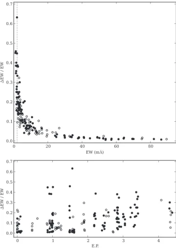
Lines with very small EW’s (<5 mA) are more susceptible to

errors in continuum placement than larger lines. Such errors can impact the determination of stellar parameters and element abundances. To better understand this, we measured minimum and maximum EWs for each line corresponding to the minimum and maximum values of the continuum. Half the difference between these is taken as the measurement

uncertainty (ΔEW), which is also given in Table 2 for each

line. ΔEW ranges from 0.3 to 2.0 mÅ, with a mean of

0.6 mÅ(σ = 0.2 mÅ). Figure 1 plots the quantity ΔEW/EW

versus EW and line excitation potential(EP). As can be seen,

most lines have an uncertainty of less then 20%, but the smallest lines can have uncertainties as large as 63%. The

bottom panel of Figure 1 shows the potential impact of

measurement uncertainties on determination of stellar effective

temperature, as the FeIlines(solid circles) show a slight trend

of increasing EW uncertainty with increasing EP. We explore

this in more detail in Section3.2.

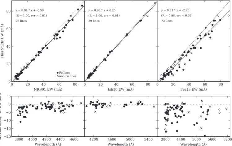
Figure2shows our EW measures compared to those of three

studies from the literature for lines in common: NRB01,

Ishigaki et al.(2010, 2012, 2013)3, and Frebel et al.(2013).

Stated again, the ﬁgures of merit for the spectra in this work

and in NRB01 are 4400 and 830, respectively. The Subaru

HDS spectrum used in Ishigaki et al.(2010,2012,2013) has

F≈ 2360, while the Magellan-MIKE spectrum of Frebel et al.

(2013) has F ≈ 490. Characteristics of these spectra are also

given in Table1for comparison.

We have a total of 75 lines in common with the line list of

NRB01 (left panels of Figure 2). Our EW measures are

generally smaller than theirs (by ∼2 mÅ), but agreement is

good for the weaker lines. For 17 lines, the difference between

our measures and those of NRB01 is 5 mÅ or more. The

bottom left panel of Figure 2 shows that 12 of these

(predominantly FeI) lines are located in the region of

3750–3950 Å. This portion of the spectrum is dominated by

very strong Balmer absorption lines, which in a star of this temperature have very extended wings. Visual inspection of the

lines with the largest measurement differences conﬁrm that the

majority of them are located in the wings of these strong absorption lines, indicating that the measurement differences could be due to differences in the continuum normalization.

2

http://www.eso.org/sci/observing/phase3.html

3

Although the results of Ishigaki et al. (2012, 2013) appear separate

from Ishigaki et al.(2010), they all use the same Subaru HDS spectrum of

CD−24°17504. Therefore, we consider the EW measures from all three studies together.

(5)

Table 2

Equivalent Widths of CD−24°17504

Species λ (Å) EP log gf EW(mÅ) ΔEW (mÅ) logϵ(X)a _UL_ﬂagb

LiI 6707.800 0.00 0.170 18.5 2.0 1.99 0 CH 4313 K K syn K 6.15 0 CH 4323 K K syn K 6.08 0 NaI 5889.950 0.00 0.108 26.6 1.7 2.61 0 NaI 5895.924 0.00 −0.194 14.6 1.5 2.59 0 MgI 4057.505 4.35 −0.890 2.1 0.5 4.43 0 MgI 4167.271 4.35 −0.710 4.2 0.8 4.55 0 MgI 4702.990 4.33 −0.380 8.8 1.0 4.53 0 MgI 5172.684 2.71 −0.450 75.2 1.2 4.55 0 MgI 5183.604 2.72 −0.239 89.4 1.6 4.60 0 MgI 5528.405 4.34 −0.498 7.4 0.4 4.56 0 AlI 3944.010 0.00 −0.620 syn K 2.47 0 AlI 3961.520 0.01 −0.340 24.6 1.1 2.35 0 AlI 3961.520 0.01 −0.340 syn K 2.40 0 SiI 3905.523 1.91 −1.092 52.6 1.3 4.19 0 SiI 3905.523 1.91 −1.092 syn K 4.20 0 CaI 4226.730 0.00 0.244 74.9 1.5 3.14 0 CaI 4283.010 1.89 −0.224 3.7 0.8 3.24 0 CaI 4318.650 1.89 −0.210 3.2 0.4 3.17 0 CaI 4425.440 1.88 −0.358 3.0 0.6 3.27 0 CaI 4434.960 1.89 −0.010 4.9 0.5 3.15 0 CaI 4435.690 1.89 −0.519 2.2 0.7 3.30 0 CaI 4454.780 1.90 0.260 8.7 0.6 3.16 0 CaI 5588.760 2.52 0.210 3.3 1.5 3.29 0 CaI 6122.220 1.89 −0.315 2.6 0.6 3.12 0 CaI 6162.170 1.90 −0.089 4.0 0.5 3.09 0 CaI 6439.070 2.52 0.470 3.3 0.6 3.00 0 ScII 4246.820 0.32 0.240 syn K −0.01 0 ScII 4314.083 0.62 −0.100 syn K −0.06 0 ScII 4324.998 0.59 −0.440 syn K −0.22 0 ScII 4400.389 0.61 −0.540 syn K −0.01 0 ScII 4415.540 0.59 −0.670 syn K 0.07 0 TiI 3989.760 0.02 −0.062 3.8 0.8 2.13 0 TiI 3998.640 0.05 0.010 5.2 0.7 2.23 0 TiI 4533.249 0.85 0.532 3.6 0.3 2.25 0 TiI 4534.780 0.84 0.336 2.1 0.2 2.19 0 TiII 3913.461 1.12 −0.420 22.7 1.0 1.94 0 TiII 4012.396 0.57 −1.750 4.2 0.6 1.89 0 TiII 4163.634 2.59 −0.400 1.8 0.3 2.03 0 TiII 4290.219 1.16 −0.930 7.6 0.4 1.88 0 TiII 4300.049 1.18 −0.490 16.4 1.0 1.85 0 TiII 4395.031 1.08 −0.540 19.4 1.1 1.89 0 TiII 4399.765 1.24 −1.190 3.5 0.3 1.85 0 TiII 4417.714 1.17 −1.190 3.6 0.4 1.79 0 TiII 4443.801 1.08 −0.720 14.9 0.6 1.92 0 TiII 4450.482 1.08 −1.520 2.9 0.6 1.95 0 TiII 4468.517 1.13 −0.600 15.0 0.8 1.85 0 TiII 4501.270 1.12 −0.770 12.7 0.7 1.92 0 TiII 4533.960 1.24 −0.530 13.4 0.5 1.82 0 TiII 4563.770 1.22 −0.960 9.1 0.5 2.03 0 TiII 4571.971 1.57 −0.320 12.7 0.5 1.88 0 TiII 5188.687 1.58 −1.050 2.2 0.4 1.79 0 CrI 4254.332 0.00 −0.114 19.3 0.5 2.13 0 CrI 4274.800 0.00 −0.220 16.6 0.7 2.16 0 CrI 4289.720 0.00 −0.370 13.8 0.6 2.20 0 CrI 5206.040 0.94 0.020 7.0 0.7 2.30 0 CrI 5208.419 0.94 0.160 10.2 0.6 2.35 0 MnI 4030.753 0.00 −0.480 syn K 2.00 0 MnI 4033.062 0.00 −0.618 syn K 2.04 0 MnI 4034.483 0.00 −0.811 syn K 2.05 0 FeI 3786.677 1.01 −2.185 3.1 0.6 4.03 0 FeI 3787.880 1.01 −0.838 38.1 0.6 4.05 0 FeI 3805.343 3.30 0.313 7.0 0.5 4.00 0 FeI 3815.840 1.48 0.237 64.5 1.1 4.04 0

(6)

Table 2 (Continued)

Species λ (Å) EP log gf EW(mÅ) ΔEW (mÅ) logϵ(X)a ULﬂagb

FeI 3820.425 0.86 0.157 82.0 0.8 4.12 0 FeI 3824.444 0.00 −1.360 61.3 0.6 4.23 0 FeI 3825.881 0.91 −0.024 70.1 0.7 4.00 0 FeI 3827.823 1.56 0.094 50.1 0.8 3.91 0 FeI 3839.256 3.05 −0.330 2.6 0.4 3.96 0 FeI 3840.438 0.99 −0.497 44.6 0.6 3.84 0 FeI 3841.048 1.61 −0.044 41.1 0.7 3.87 0 FeI 3846.800 3.25 −0.020 3.8 0.8 4.00 0 FeI 3849.967 1.01 −0.863 38.1 0.7 4.06 0 FeI 3850.818 0.99 −1.745 10.2 0.8 4.12 0 FeI 3852.573 2.18 −1.180 2.7 0.5 4.01 0 FeI 3856.372 0.05 −1.280 64.3 0.8 4.28 0 FeI 3859.911 0.00 −0.710 86.3 0.6 4.32 0 FeI 3865.523 1.01 −0.950 33.9 0.7 4.06 0 FeI 3867.216 3.02 −0.450 3.1 0.5 4.13 0 FeI 3878.018 0.96 −0.896 37.6 0.5 4.04 0 FeI 3878.573 0.09 −1.380 57.1 0.7 4.20 0 FeI 3895.656 0.11 −1.668 38.2 0.7 4.03 0 FeI 3899.707 0.09 −1.515 48.9 1.0 4.11 0 FeI 3902.946 1.56 −0.442 33.1 0.7 4.03 0 FeI 3917.181 0.99 −2.155 4.3 0.5 4.11 0 FeI 3920.258 0.12 −1.734 41.0 0.8 4.16 0 FeI 3922.912 0.05 −1.626 48.9 0.9 4.18 0 FeI 3977.741 2.20 −1.120 3.5 0.6 4.10 0 FeI 4005.242 1.56 −0.583 29.8 0.8 4.08 0 FeI 4021.866 2.76 −0.730 2.7 0.6 4.10 0 FeI 4045.812 1.49 0.284 69.4 0.8 4.15 0 FeI 4062.441 2.85 −0.860 2.0 0.5 4.17 0 FeI 4063.594 1.56 0.062 57.2 0.7 4.10 0 FeI 4067.978 3.21 −0.470 1.6 0.4 4.01 0 FeI 4071.738 1.61 −0.008 52.3 0.7 4.08 0 FeI 4076.629 3.21 −0.370 1.6 0.3 3.91 0 FeI 4132.058 1.61 −0.675 25.3 0.9 4.11 0 FeI 4134.678 2.83 −0.649 3.6 0.5 4.20 0 FeI 4136.998 3.42 −0.450 1.4 0.5 4.12 0 FeI 4143.414 3.05 −0.200 5.3 0.5 4.13 0 FeI 4143.868 1.56 −0.511 33.6 0.7 4.09 0 FeI 4147.669 1.48 −2.071 1.8 0.4 4.09 0 FeI 4153.899 3.40 −0.320 1.8 0.5 4.08 0 FeI 4154.498 2.83 −0.688 2.0 0.5 3.98 0 FeI 4154.805 3.37 −0.400 1.5 0.6 4.05 0 FeI 4156.799 2.83 −0.808 2.3 0.7 4.16 0 FeI 4157.780 3.42 −0.403 2.6 0.5 4.34 0 FeI 4174.913 0.91 −2.938 1.3 0.5 4.26 0 FeI 4181.755 2.83 −0.371 6.4 0.7 4.19 0 FeI 4184.892 2.83 −0.869 2.0 0.4 4.16 0 FeI 4187.039 2.45 −0.514 7.9 0.5 4.08 0 FeI 4187.795 2.42 −0.510 7.8 0.6 4.04 0 FeI 4191.430 2.47 −0.666 6.1 0.3 4.13 0 FeI 4195.329 3.33 −0.492 1.8 0.5 4.18 0 FeI 4199.095 3.05 0.156 9.5 0.8 4.05 0 FeI 4202.029 1.49 −0.689 29.6 0.9 4.10 0 FeI 4216.184 0.00 −3.357 2.8 0.4 4.17 0 FeI 4222.213 2.45 −0.914 3.2 0.6 4.06 0 FeI 4227.427 3.33 0.266 8.2 0.7 4.12 0 FeI 4233.603 2.48 −0.579 6.5 0.7 4.08 0 FeI 4238.810 3.40 −0.233 2.1 0.7 4.05 0 FeI 4247.426 3.37 −0.240 2.7 0.9 4.15 0 FeI 4250.119 2.47 −0.380 9.3 0.7 4.04 0 FeI 4250.787 1.56 −0.713 24.9 0.5 4.08 0 FeI 4260.474 2.40 0.077 24.2 0.7 4.03 0 FeI 4271.154 2.45 −0.337 11.6 0.8 4.09 0 FeI 4271.760 1.49 −0.173 53.8 0.6 4.15 0 FeI 4282.403 2.18 −0.779 7.3 0.5 4.06 0

(7)

Table 2 (Continued)

FeI 4325.762 1.61 0.006 53.7 0.3 4.07 0 FeI 4352.735 2.22 −1.290 2.2 0.9 4.05 0 FeI 4375.930 0.00 −3.005 5.9 0.5 4.13 0 FeI 4383.545 1.48 0.200 69.4 0.7 4.17 0 FeI 4404.750 1.56 −0.147 52.4 0.7 4.14 0 FeI 4415.122 1.61 −0.621 29.9 0.5 4.13 0 FeI 4427.310 0.05 −2.924 6.7 0.6 4.16 0 FeI 4442.339 2.20 −1.228 3.1 0.6 4.16 0 FeI 4447.717 2.22 −1.339 2.5 0.4 4.15 0 FeI 4459.118 2.18 −1.279 3.3 0.6 4.18 0 FeI 4461.653 0.09 −3.194 4.0 0.7 4.22 0 FeI 4466.552 2.83 −0.600 2.5 1.0 3.95 0 FeI 4476.019 2.85 −0.820 2.9 0.6 4.27 0 FeI 4528.614 2.18 −0.822 7.6 0.6 4.10 0 FeI 4531.148 1.48 −2.101 1.7 0.5 4.05 0 FeI 4602.941 1.49 −2.208 1.2 0.6 4.00 0 FeI 4871.318 2.87 −0.362 4.3 0.6 3.99 0 FeI 4890.755 2.88 −0.394 4.3 0.5 4.03 0 FeI 4891.492 2.85 −0.111 9.1 0.4 4.07 0 FeI 4903.310 2.88 −0.926 1.3 0.5 4.03 0 FeI 4918.994 2.85 −0.342 5.1 0.6 4.03 0 FeI 4920.503 2.83 0.068 13.1 0.7 4.06 0 FeI 5012.068 0.86 −2.642 1.9 0.9 4.03 0 FeI 5083.339 0.96 −2.842 1.7 0.7 4.27 0 FeI 5171.596 1.49 −1.721 4.3 0.7 4.05 0 FeI 5192.344 3.00 −0.421 3.2 0.5 4.02 0 FeI 5194.942 1.56 −2.021 1.9 1.2 4.05 0 FeI 5232.940 2.94 −0.057 8.8 0.6 4.07 0 FeI 5266.555 3.00 −0.385 3.5 0.7 4.03 0 FeI 5269.537 0.86 −1.333 34.4 1.0 4.20 0 FeI 5328.039 0.92 −1.466 13.5 0.6 3.81 0 FeI 5371.489 0.96 −1.644 8.9 0.7 3.81 0 FeI 5383.369 4.31 0.645 2.7 0.7 4.07 0 FeI 5397.128 0.92 −1.982 9.8 1.0 4.16 0 FeI 5405.775 0.99 −1.852 11.0 0.6 4.15 0 FeI 5415.199 4.39 0.643 2.5 0.5 4.11 0 FeI 5424.068 4.32 0.520 3.5 1.1 4.32 0 FeI 5429.696 0.96 −1.881 11.1 1.0 4.16 0 FeI 5434.524 1.01 −2.126 5.6 1.1 4.12 0 FeI 5446.917 0.99 −1.910 10.7 1.3 4.20 0 FeI 5455.609 1.01 −2.090 7.0 0.7 4.19 0 FeI 5497.516 1.01 −2.825 1.0 0.5 4.05 0 FeI 5506.779 0.99 −2.789 1.6 0.3 4.20 0 FeI 5586.756 3.37 −0.144 3.2 0.8 4.07 0 FeI 5615.644 3.33 0.050 4.7 0.8 4.02 0 FeII 4233.170 2.58 −1.970 6.4 1.3 4.08 0 FeII 4522.630 2.84 −2.250 2.9 0.7 4.21 0 FeII 4583.840 2.81 −1.930 5.0 0.7 4.11 0 FeII 4923.930 2.89 −1.320 12.4 0.8 4.00 0 FeII 5018.450 2.89 −1.220 16.4 1.1 4.04 0 CoI 3845.468 0.92 0.010 7.6 1.0 2.01 0 CoI 3873.120 0.43 −0.660 9.0 0.9 2.31 0 CoI 3995.306 0.92 −0.220 7.2 0.8 2.20 0 CoI 4121.318 0.92 −0.320 4.8 0.6 2.10 0 NiI 3783.520 0.42 −1.420 16.2 1.1 3.20 0 NiI 3807.140 0.42 −1.220 19.6 0.7 3.09 0 NiI 3858.301 0.42 −0.951 32.6 0.8 3.15 0 NiI 5476.900 1.83 −0.890 4.3 0.4 3.19 0 ZnI 4810.528 4.08 −0.137 3.1 1.0 2.15 0 SrII 4077.714 0.00 0.150 5.5 0.6 −1.81 0 SrII 4077.714 0.00 0.150 syn K −1.82 0 SrII 4215.524 0.00 −0.180 3.1 0.7 −1.75 0 SrII 4215.524 0.00 −0.180 syn K −1.80 0 YII 3788.694 0.10 −0.140 <1.0 K <−1.36 1

(8)

The remainingﬁve lines with large measurement differences were not located near any strong absorption features. In each case, we could not reduce the EW measurement difference by adjustment of the continuum; to make the lines as strong as

measured by NRB01required measuring the line well above

the location of the continuum. We therefore attribute the measurement differences to S/N differences.

The right panels of Figure2compare our EW measures with

those measured in a MIKE spectrum of CD −24°17504 from

our earlier work (Frebel et al. 2013). Here, the agreement is

less good, with a larger mean offset(5.4 mÅ) and substantially

larger scatter. We inspected each line for which the EW

difference was larger than 3 mÅ(45 lines) in the MIKE

spectrum from Frebel et al.(2013), which has both lower S/N

and lower resolution than in this work(Table1). Only nine of

these lie near strong Balmer features. For 14 lines, we found that the EW values were consistent with each other considering the S/N of the region; that is, that slight adjustments of the continuum level within its uncertainty got the EW measures to agree. For 15 further lines, similar adjustments decreased the EW discrepency by 50% or more. For some remaining lines, EW discrepencies could not be decreased.

Finally, the middle panels compare our measures to those in

Ishigaki et al. (2010, 2012, 2013). Though we only have

39 lines in common, this study is in a sense most similar to ours in that their analysis was based on data superior in resolution

(R ∼ 55,000) and of high S/N (∼250; Table1). As can be seen,

agreement is excellent, with a mean offset of −0.2 mÅ. In

summary, the differences in EW measures among these different studies is representative of the varying quality of the data they came from.

3.2. Determination of Stellar Parameters

For this work, we make use of the Castelli–Kurucz grid of

1D plane-parallel model atmospheres(Castelli & Kurucz2004)

with no-overshoot and the local thermodynamic equilibrium (LTE) analysis code MOOG (2011 May version, Sneden

1973) that includes treatment of Rayleigh scattering (Sobeck

et al. 2011). Stellar parameters for CD −24°17504 were

determined via classical spectroscopic techniques which use

the EWs of FeIand FeIIlines described in the previous section.

Effective temperature was determined by reducing any trend of

FeI line abundance with EP, and microturbulent velocity

was adjusted to remove FeI line abundance trends with

reduced EW. Surface gravity, log g, was adjusted until the

average FeIand FeIIagreed within 0.05 dex. The metallicity of

the model atmosphere ([M/H]) was also adjusted as needed.

This process was iterated upon until all three requirements were

satisﬁed, and then we applied the empirical correction to

Teffdescribed in Frebel et al. (2013). The resulting stellar

parameters are Teff= 6228 K, log g = 3.90, vt= 1.25 km s−1,

and[Fe/H] = −3.41 (σ = 0.10) dex (Table3).

Based on an analysis of a MIKE spectrum of CD−24°17504

described earlier, we found Teffand vtvalues in good agreement

with those found here: 6259 K and 1.40 km s−1, respectively

(Frebel et al.2013). However, the surface gravity in that work

was 0.25 dex lower (log g = 3.65), and [Fe/H] was 0.18 dex

higher(−3.23). In Frebel et al. (2013), the FeIIabundance was

based on measures of two lines in CD−24°17504, the EWs of

both being∼50% larger than found in this study (see previous

Table 2 (Continued)

ZrII 4208.977 0.71 −0.460 <1.0 K <0.08 1 BaII 4554.033 0.00 0.163 <1.0 K <−2.28 1 LaII 4123.220 0.32 0.130 <1.0 K <−1.08 1 EuII 4129.700 0.00 0.220 <1.0 K <−1.73 1 Notes. a LTE abundance. b

Upper limitﬂag: 1 = yes, 0 = no.

Figure 1. Fraction EW uncertainty (ΔEW/EW) as a function of line strength (top panel) and line EP (bottom panel). FeIand FeIIlines are indicated by black circles, and non-Fe species are given as open circles. To guide the eye, the dotted line in the top panel indicates a line strength of 2 mÅ.

(9)

section). To investigate the matter, we adjusted the measures of these two lines in their MIKE spectrum within comfortable limits of the noise level and repeated the stellar parameter

determination, resulting in parameters Teff = 6259 K,

log g = 4.35, vt = 1.2 km s−1, and [Fe/H] = −3.22. This

0.7 dex adjustment to surface gravity illustrates the necessity of

having several well-measured FeII lines for spectroscopic

stellar parameter determination. The ∼0.2 dex higher

metalli-city compared to that found in this study can likewise be attributed to systematically larger EWs.

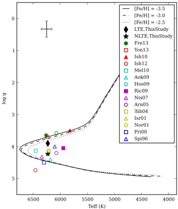
Numerous stellar parameter determinations for CD−24°17504

based on different techniques can be found in the literature.

Figure 3 shows the position of CD −24°17504 in the

Hertzsprung–Russell diagram using stellar parameters from

various studies, which are also listed in Table3. Filled symbols

represent studies that determined stellar parameters spectro-scopically, similar to that described above. Open symbols

indicate studies that determined Teffvia photometry and

color-temperature calibrations, or viaﬁtting the wings of Balmer lines.

In these cases, log g was either determined via matching to

theoretical isochrones or by ionization balance of FeI and FeII

lines. Figure 3 and Table 3 clearly show the range of stellar

parameters these same few methods, used by different authors,

provide. Indeed, CD −24°17504 can be classiﬁed as either a

main sequence dwarf star or a subgiant.

It is also well established that the assumption of LTE can introduce systematic offsets into a classical spectroscopic analysis, and that these systematics increase with decreasing

stellar metallicity and decreasing log g(e.g., Thévenin &

Idiart 1999; Asplund 2005; Lind et al. 2012). To mitigate

these effects, we determined stellar parameters for

CD−24°17504 following a method described in Ruchti et al.

(2013) and starting with our empirically calibrated

spectro-scopic Teff(6228 K).4 We then determined Δ[Fe/H] (NLTE

−LTE) for FeI lines in our line list that were present in the

INSPECT database,5 adopting Teff = 6228 K, log g = 4.0,

[Fe/H] = −3.4, and vt = 1.25 km s−1(Bergemann et al.

2012b; Lind et al. 2012). For the 18 FeI lines, the average

Δ[Fe/H] = +0.12 dex (σ = 0.04). Therefore, [FeI/H]_LTE= −3.41

corresponds to[FeI/H]_NLTE= −3.29. Next, log g was adjusted to

achieve [FeII/H] = −3.29, and v_twas adjusted to remove any

trends of FeI abundance with line strength. The resulting

“NLTE” stellar parameters are Teff = 6228 K, log g = 4.23,

vt= 1.00 km s−1, and[Fe/H] = −3.29 (Table3).

The LTE and “NLTE” parameters determined here for

CD−24°17504 are indicated by a black diamond and black star

in Figure 3, respectively. As can be seen, CD −24°

17504 appears to be a dwarf star or a subgiant star depending

on the assumption of LTE for FeIlines in the determination of

log g via ionization balance. Our“NLTE” parameters are more

consistent with those found photometrically, the majority of

which indicate CD−24°17504 is a dwarf star with log g > 4.

For the rest of this paper, we will mostly focus on the LTE parameters and subsequent element abundances for comparison

Figure 2. Comparison of EWs measured in this study to those in the literature. In the top panels, dotted lines indicate a 1:1 correlation, while solid lines are lines of bestﬁt through the data. FeIand FeIIlines are indicated byﬁlled circles. The bottom panels show the difference between EW measures as a function of wavelength.

4

Recall that this calibration places spectroscopically determined Teffvalues

on a rough “photometric” scale, and that this correction increases with decreasing Teff(and decreasing log g)—similar to the direction that NLTE–

LTE differences increase. Therefore this empirical calibration “softens the blow” of using purely spectroscopic techniques.

5

(10)

to literature values (which by and large assume LTE), but we

will include abundances determined with the “NLTE”

parameters for reference. Additional NLTE corrections to individual elements will also be discussed were necessary and available. Finally, we note this analysis did not consider

possible 1D–3D effects and the possible systematic biases

introduced by our assumption of plane-parallel model atmo-spheres. 3D effects can be large for stars of this metallicity, but

exploration of them except for speciﬁc elements is beyond the

scope of this paper.

3.3. Element Abundance Analysis

Abundances for the following elements were determined

using measured EWs and the LTE and“NLTE” sets of stellar

parameters described above: NaI, MgI, SiI, CaI, TiI, TiII, CrI,

CoI, NiI, and ZnI. Each line measurement was visually

inspected and strong outliers were removed. Spectrum

synth-esis was used to determine abundances for Li, C, ScII, MnI,

and SrII. Sets of three synthetic spectra of varying element

abundance were generated using MOOG and plotted over the observed spectrum. The synthetic spectra were convolved with a Gaussian to match the resolution of the data and the continuum level was adjusted where necessary. The element abundance was then varied until the best match was found. This was done by visually evaluating the residuals of the (synthetic-observed) data.

Upper limits to element abundances were calculated based

on the noise level of the spectrum. Theσ of the noise level can

be assessed using the Cayrel formula: σ ≈ 1.5 × (S/N)−1 ×

( FWHM´dx), where S/N is the signal-to-noise ratio,

FWHM is the typical full width at half maximum of absorption

lines in that part of the spectrum, and δx is the spectral

dispersion(Cayrel et al.1988). Typical values were ∼0.15 mÅ.

The corresponding 3σ upper limit EW of 0.5 mÅ is comparable

to the mean ΔEW uncertainty of 0.6 mÅ discussed earlier.

However, we have opted to set the upper limit EW to 1 mÅ, the

minimum accepted value for detected lines (Table 2). This

value was used to determine upper limits to the abundances of

YII (3788 Å), ZrII (4209 Å), BaII (4554 Å), LaII (4123 Å),

and EuII(4129 Å). The element abundances corresponding to

these upper limit EWs were found using either the“blends” or

“abﬁnd” routine in MOOG, for lines with and without

hyperﬁne or isotopic splitting, respectively. In the case of Ba,

we adopted the r-process only isotopic ratio. Individual line

LTE abundances are given in Table2.

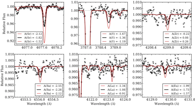
Figure 4 shows the results of this upper limit analysis, as

well as spectrum synthesis of the region around the SrII4077 Å

feature. For the Sr synthesis, synthetic spectra with logϵ(Sr) ±

0.3 dex around the best-ﬁt abundance are shown by red lines.

For all the other species, synthetic spectra with the abundances determined from the 1 mÅ EW upper limits are shown as black solid lines, while the red lines represent synthetic spectra with abundances found using EWs of 0.5 and 1.5 mÅ. As can be seen, 1 mÅ is a reasonable upper limit in each region of the spectrum.

Table 3

Atmospheric Parameters for CD−24°17504 in this Study and in the Literature

Teff log g vt [Fe/H]

(K) (dex) (km s−1₎ _(dex) _Method _References

6228 3.90 1.25 −3.41 speca, LTE This Study

6228 4.23 1.00 −3.29 speca,

NLTE

This Study 6259 3.65 1.40 −3.23 speca Frebel et al.(2013)

6236 3.70 1.60 −3.23 phot Yong et al.(2013a)

5821 3.50 1.22 −3.66 spec Ishigaki et al.(2010)

6456 4.74 1.50 −3.20 comb Ishigaki et al.(2012)

6451 4.13 K −3.34 phot Meléndez et al.(2010)

6180 4.40 1.50 −3.40 balm Aoki et al.(2009)

6070 3.57 1.30 −3.35 comb Hosford et al.(2009)

5942 4.05 1.50 −3.42 spec Rich &

Boes-gaard(2009)

6338 4.32 1.50 −3.21 balm Nissen et al.(2007)

6070 4.20 1.80 −3.45 phot Arnone et al.(2005)

6212 4.13 1.00 −2.99 phot Bihain et al.(2004)

6212 4.13 K −3.32 phot Israelian et al.(2001)

6070 3.60 1.40 −3.37 comb Norris et al.(2001)

6300 4.50 1.00 −3.30 phot Primas et al.(2000)

6100 4.00 1.50 −3.70 balm Spite et al.(1996)

Notes. Methods for determining stellar parameters range from classical spectroscopic methods(“spec”), use of color-temperature relations (“phot”), or ﬁtting of Balmer line absorption wings (“balm”). In the latter two methods, log g is often determined by comparison to theoretical isochrones, but in some cases, is determined by ionization balance. These cases are noted as“comb,” for combination of methods.

a

Parameters determined spectroscopically, but with correction applied to Teff.

See text for more information.

Figure 3. Location of CD −24°17504 in the Hertzsprung–Russell diagram using stellar parameters from different studies. For reference, 12 Gyr Yale-Yonseii isochrones with[α/Fe] = +0.40 and [Fe/H] = −2.5, −3.0, and −3.5 are shown as dotted, dashed, and solid lines, respectively(Kim et al.2002). Filled

symbols indicate that stellar parameters were determined spectroscopically; open symbols indicate other methods were used. The parameters found in this work are indicated by aﬁlled diamond (LTE) and star (“NLTE”), respectively. See text for details. Note that the literature results assume LTE; references are given in Table3.

(11)

It has been noted in the literature that the MnI resonance lines at 4030 Å indicate systematically lower Mn abundances

than do weaker non-resonance lines (Cayrel et al. 2004; Lai

et al.2008). Our investigations of these offsets in HD 122563

and HD 140283 found an offset of +0.30 dex(in the sense

non-resonance minus non-resonance), in agreement with literature

studies. Therefore, we have corrected the abundances

deter-mined from MnI 4030 Å, 4033 Å, and 4034 Å by +0.30 dex.

The individual Mn line abundances in Tables 2 include this

offset. Bergemann & Gehren (2008) have shown that this

0.3 dex offset can be attributed to NLTE effects on the resonance lines.

Abundance results are presented in Table 6 adopting the

LTE stellar parameters, while the results of the “NLTE”

analysis are shown in Table 7. The adopted solar abundances

are those of Asplund et al.(2009).

3.4. Analysis of the Uncertainties

We evaluated the uncertainties in the stellar parameters of

CD−24°17504 in the following way. Teffand vtwere adjusted

until slopes were introduced into relations of FeI line

abundance with EP and reduced EW that exceeded tolerable

levels given the 1σ dispersion in FeIline abundances. Surface

gravity was adjusted until[FeII/H] − [Fe/H] = (s_{Fe I}2 +s_{Fe II}2 )1 2.

The results are ΔTeff = 60 K, Δlog g = 0.30, and

Δvt = 0.1 km s−1. These values are consistent with those

found using the empirical relations of Roederer et al. (2014):

ΔTeff = 61 K (40 K), Δvt = 0.05 km s−1(0.15 km s−1) for

the subgiant (main-sequence) star relations. Finally, we set

Δ[M/H] = σFeI.

We evaluated the sensitivity of these parameters to uncertainties in EW measures in a Monte Carlo fashion.

Starting with the EW measures in Table 2, we generated

Gaussian distributions of EWs for each line with the FWHM

equal to the line’s ΔEW. We then randomly selected an EW

from these distributions and generated 10 sets of EW measures.

For the smallest FeIlines, if the resulting EW was smaller than

1 mÅ, it was excluded(generally no more than 2−3 lines were

excluded). Starting from the original stellar parameters (before

application of the Teffcorrection), Teff, vtand log g were varied

to establish ionization and excitation balance and to remove

abundance trends with line strength. The empirical

Teffcorrection was then applied andﬁnal adjustments to log g,

vt, and [M/H] were performed. The difference between the

resulting parameters and the LTE parameters in Table 3 for

each of the 10 trials is given in Table 4. Considering the

Figure 4. Portions of the spectrum of CD −24°17504 at the locations of various neutron-capture element absorption features. The only element detected, Sr, was analyzed with spectrum synthesis. The best-ﬁt synthetic spectrum is indicated by a black solid line, with spectra illustrating logϵ(Sr) ≡ A(Sr) ± 0.3 dex are shown as red lines. For the other elements, synthetic spectra with element abundances determined adopting an EW upper limit of 1 mÅ are given by black lines, with red lines representing synthetic spectra with abundances determined using EWs of 0.5 and 1.5 mÅ.

Table 4

Uncertainties in Stellar Parameters Due to Errors in FeI, FeIIEWs

ΔTeff Δlog g Δvt Δ[Fe/H]

Run (K) (dex) (km s−1) (dex) # FeI # FeII

01 −68 −0.18 +0.00 −0.04 112 5 02 +76 −0.02 +0.06 +0.07 112 5 03 −67 −0.24 +0.06 −0.06 109 5 04 +13 +0.02 +0.05 +0.01 110 5 05 −51 −0.25 +0.00 −0.03 112 5 06 +123 +0.48 +0.04 +0.10 110 5 07 +37 +0.09 +0.08 +0.02 112 5 08 −71 −0.05 −0.09 −0.04 110 5 09 −6 −0.03 +0.08 −0.01 110 5 10 −74 −0.13 −0.02 −0.05 113 5 Ave. 59 0.15 0.05 0.04 K K σ 34 0.15 0.03 0.03 K K

(12)

magnitudes of the differences, they are on average 59

(σ = 34) K for Teff, 0.15 (σ = 0.15) dex for log g, 0.05

(σ = 0.03) km s−1_{for v}

t, and 0.04 (σ = 0.03) dex for [Fe/H].

These values along with the uncertainties in the previous paragraph were added in quadrature to determine the total

uncertainties in the spectroscopic parameters: 84 K for Teff,

0.34 dex for log g, 0.11 km s−1for vt, and 0.11 dex for[M/H].

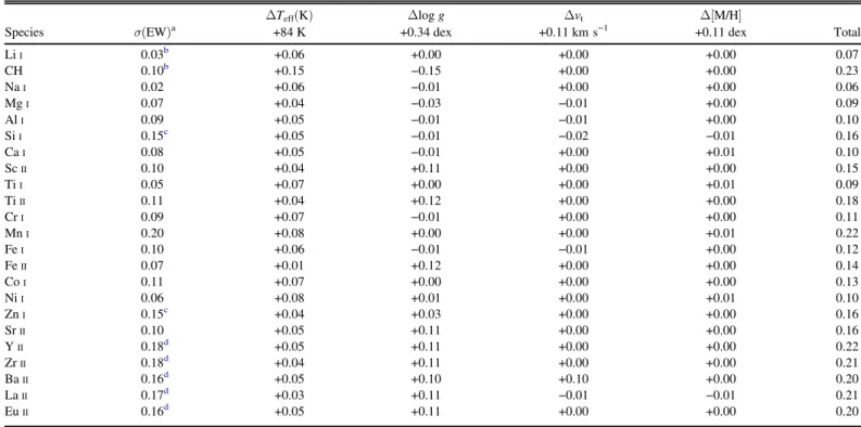
The sensitivity of element abundances to these parameter uncertainties were determined by varying each parameter by its

uncertainty independently. Table 5 gives the abundance

uncertainties for each element.

For the non-Fe species, we determined the uncertainty in the abundance due to EW error by using the 10 variations of the line list and determined individual line abundances using the LTE stellar parameters. The mean element abundances were

then compared to those in Table 6. Typical differences were

0.02 to 0.03 dex, but were as large as 0.14 dex in the case of the

single ZnIline measured. We take the maximum of either this

difference or the standard deviation of the line abundances in

Table 6 as the element abundance sensitivity to EW

uncertainty. The total sensitivity of element abundances to stellar parameter and EW uncertainties was found by adding all the uncertainties in quadrature, as given in the last column of

Table5.

4. RESULTS AND DISCUSSION 4.1. Comparison to Literature Results

In this section, we compare our abundance results to those of

different studies from the literature: NRB01, Ishigaki et al.

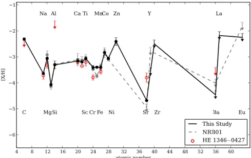
(2010, 2012, 2013), and Frebel et al. (2013). Figure 5

illustrates the overall abundance([X/H]) pattern found here and

in NRB01, with their abundances placed on our solar abundance scale. We also show for comparison a star with similar stellar parameters from the sample of Yong et al. (2013a). This star, HE 1346−0427, has Teff/log g/vt/[Fe/H] =

6255/3.69/1.40/−3.57, and has an abundance pattern typical for

stars of its metallicity(see Figure 43 of Yong et al.2013a). As

can be seen, CD−24°17504 has a similar abundance pattern to

this star for elements up to the Fe-peak, apart from C and Al,

for which HE 1346−0427 only has upper limits. This conﬁrms

that apart from C and the neutron-capture species, CD −24°

17504 also has element abundances typical for stars of its metallicity.

For the elements with atomic number Z < 29 in common, the

agreement of our results withNRB01is excellent, apart from

Mn.NRB01measured only the Mn resonance lines, and do not include any systematic correction to the abundances. The ∼0.3 dex discrepancy between their abundance and ours can be entirely explained by the lack of such correction. For the

neutron-capture elements,NRB01provided upper limits for Sr,

Y, Ba, and Eu. For all but Sr, we have been able to lower the upper limits for these species by a minimum of 0.40 dex, or a factor of 2.5. Our detections of the 4077 and 4215 Å features

yield a larger Sr abundance than found by NRB01by nearly

0.2 dex. We can reproduce their upper limit using their stellar parameters.

Figure6illustrates the comparison to NRB01another way,

along with comparisons to Frebel et al.(2013), Ishigaki et al.

(2010, 2012, 2013; placed on our abundance scale, again

Table 5

Log(ϵ) Abundance Uncertainties due to Atmospheric Parameters

ΔTeff(K) Δlog g Δvt Δ[M/H]

Species σ(EW)a +84 K +0.34 dex +0.11 km s−1 +0.11 dex Total

LiI 0.03b +0.06 +0.00 +0.00 +0.00 0.07 CH 0.10b +0.15 −0.15 +0.00 +0.00 0.23 NaI 0.02 +0.06 −0.01 +0.00 +0.00 0.06 MgI 0.07 +0.04 −0.03 −0.01 +0.00 0.09 AlI 0.09 +0.05 −0.01 −0.01 +0.00 0.10 SiI 0.15c +0.05 −0.01 −0.02 −0.01 0.16 CaI 0.08 +0.05 −0.01 +0.00 +0.01 0.10 ScII 0.10 +0.04 +0.11 +0.00 +0.00 0.15 TiI 0.05 +0.07 +0.00 +0.00 +0.01 0.09 TiII 0.11 +0.04 +0.12 +0.00 +0.00 0.18 CrI 0.09 +0.07 −0.01 +0.00 +0.00 0.11 MnI 0.20 +0.08 +0.00 +0.00 +0.01 0.22 FeI 0.10 +0.06 −0.01 −0.01 +0.00 0.12 FeII 0.07 +0.01 +0.12 +0.00 +0.00 0.14 CoI 0.11 +0.07 +0.00 +0.00 +0.00 0.13 NiI 0.06 +0.08 +0.01 +0.00 +0.01 0.10 ZnI 0.15c +0.04 +0.03 +0.00 +0.00 0.16 SrII 0.10 +0.05 +0.11 +0.00 +0.00 0.16 YII 0.18d +0.05 +0.11 +0.00 +0.00 0.22 ZrII 0.18d +0.04 +0.11 +0.00 +0.00 0.21 BaII 0.16d +0.05 +0.10 +0.10 +0.00 0.20 LaII 0.17d +0.03 +0.11 −0.01 −0.01 0.21 EuII 0.16d +0.05 +0.11 +0.00 +0.00 0.20 Notes. a

The maximum of the standard deviation of individual line element abundances or the abundance sensitivity to EW uncertainties.

b

Sensitivity of abundance to continuum placement.

c

Value given to measures based on one line.

d

(13)

relative to our LTE abundances). Here we distinguish between

the results of Ishigaki et al.(2010) from the more recent papers,

as the analyses(of the same spectrum) are independent and use

very different stellar parameters. In Figure6, the difference in

log ϵ(X), in the sense (This Study—Literature) is shown for

each element. Again, the good agreement with NRB01(black

squares) is obvious, apart from the elements already discussed.

Generally, our element abundances are lower than those

found by Frebel et al.(2013) and Ishigaki et al. (2012,2013),

and higher than those found by Ishigaki et al. (2010). The

difference with Frebel et al.(2013) can largely be explained by

the smaller EW measures in this study. The differences with

Ishigaki et al. (2010, 2012, 2013) are likely due to the very

different atmospheric parameters used in those works (see

Figure 3). Adopting the stellar parameters of Ishigaki et al.

(2012,2013) resulted in abundances within 0.1 dex agreement

with their values. This is similarly the case when using the

Ishigaki et al. (2010) parameters, though abundance

discre-pencies greater than 0.2 dex remained for Mg and Ti.

Interestingly, Ishigaki et al. (2010) present a Ba abundance

for CD−24°17504, based on a 1 mÅ EW of the 4554 Å feature

(they do not specify it as an upper limit). We can reproduce

their abundance, logϵ(Ba) ≈ −2.8, adopting this EW and their

stellar parameters. However, as we cannot see a clear Ba absorption feature of this size in our spectrum, we prefer to determine an upper limit as already described.

4.2. Discussion of Individual Elements

To place the abundances of CD −24°17504 found in this

work in context of other known main sequence and turn-off stars of comparable metallicity, we have collected element abundances for stars having stellar paramters within the ranges

5900 K⩽ Teff⩽ 6500 K, 3.6 ⩽ log g ⩽ 4.8, and [Fe/H] ⩽ −3.0

from the works of Yong et al.(2013a), Roederer et al. (2014),

Cohen et al.(2013), and Aoki et al. (2013). We also include,

without any selection criteria, the turn-off star samples of

Bonifacio et al. (2009, 2011), Behara et al. (2010), Caffau

et al. (2011, 2013a), and Caffau et al. (2013b). In all cases,

literature abundances have been placed on the Asplund et al.

(2009) solar abundance scale.

4.2.1. Lithium

Figure 7 illustrates spectrum synthesis of the Li I 6707 Å

doublet in CD−24°17504. The measured EW of the feature is

18.5 mÅ. The lithium abundance of CD −24°17504 has been

subject to previous study (Primas et al. 2000; Meléndez &

Ramírez2004; Aoki et al.2009; Hosford et al.2009; Meléndez

et al.2010). The LTE abundance found here, logϵ(Li) = 1.99,

is in excellent agreement with that of Primas et al.(2000). As

the abundance of Li is sensitive to Teff, we see best agreement

with literature studies that adopted similar Teffvalues (that of

Primas et al. 2000is 6300 K). The Keck spectra used in this

work were analyzed in Meléndez & Ramírez (2004) and

Meléndez et al.(2010). Our measurement of the Li feature is in

excellent agreement with theirs, 18.6 mÅ, and the 0.30 dex

abundance difference can be attributed to their Teffbeing∼225

K hotter than ours.

We determined the NLTE correction to this Li abundance

using the grid of Lind et al. (2009) via the “INSPECT”

website:(NLTE−LTE) Δlogϵ(Li) = −0.05. This correction is

the same regardless of whether we use the LTE or “NLTE”

stellar parameters, as the Teffis identical in both cases.

The Li abundance patterns of unevolved extremely

metal-poor stars such as CD −24°17504 have been explored to

investigate the behavior of the Spite plateau in the low-metallicity regime, and our result does not add anything new to

the discussion (e.g., Spite & Spite 1982; Ryan et al. 2001;

Meléndez & Ramírez2004; Bonifacio et al. 2007; Meléndez

et al.2010; Sbordone et al.2010). We therefore note that our Li

abundance for CD−24°17504 is very consistent with those of

other stars of similar Teffand[Fe/H] in Sbordone et al. (2010),

and refer the reader to that paper for details (see also, e.g.,

Meléndez et al.2010).

4.2.2. Carbon

The CH G band is clearly detected in our spectrum of

CD−24°17504, as can be seen in Figure8. The best ﬁt LTE

carbon abundance based on the G band is logϵ(C) = 6.12 ±

0.05, or[C/Fe] = +1.10. Using the “NLTE” stellar parameters,

[C/Fe] = +0.83. To our knowledge, this is the ﬁrst detection

of the CH G band in this star. Fabbian et al.(2009) determined

a C abundance for CD−24°17504 based on the EW measures

of two CI lines in the infrared. They reported LTE

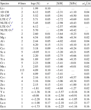
Table 6

Element Abundances for CD−24o_{17504 Based on LTE Stellar Parameters}

Species # lines logϵ(X) σ [X/H] [X/Fe] _{σ/ N}( )

LiI 1 1.99 0.10 K K K 1D CH 2 6.12 0.05 −2.31 +1.10 0.04 3D CHa 2 5.52 0.05 −2.91 +0.50 0.01 LTE CIb 2 5.71 0.05 −2.72 +0.69 0.03 NLTE CIc 2 5.45 0.05 −2.98 +0.43 0.03 LTE OIb 1 6.12 K −2.57 +0.84 K NLTE OId 1 5.70 K −2.99 +0.42 K NaI 2 2.60 0.01 −3.64 −0.23 0.01 MgI 6 4.54 0.05 −3.06 +0.34 0.02 AlI 2 2.44 0.05 −4.02 −0.61 0.04 SiI 1 4.20 0.15 −3.31 +0.10 0.15 CaI 11 3.18 0.09 −3.16 +0.24 0.03 ScII 5 −0.05 0.11 −3.20 +0.21 0.05 TiI 4 2.20 0.05 −2.75 +0.66 0.03 TiII 16 1.89 0.07 −3.06 +0.35 0.02 CrI 5 2.23 0.08 −3.41 −0.01 0.04 MnI 3 2.03 0.03 −3.40 +0.01 0.02 FeI 113 4.09 0.10 −3.41 K 0.01 FeII 5 4.09 0.07 −3.41 K 0.03 CoI 4 2.16 0.11 −2.83 +0.57 0.06 NiI 4 3.16 0.04 −3.06 +0.34 0.03 ZnI 1 2.15 0.15 −2.41 +1.00 0.15 SrII 2 −1.81 0.02 −4.68 −1.27 0.02 YII 1 <−1.36 0.18 <−3.57 <−0.16 0.18 ZrII 1 <0.08 0.18 <−2.50 <+0.91 0.18 BaII 1 <−2.28 0.16 <−4.46 <−1.05 0.16 LaII 1 <−1.08 0.17 <−2.18 <+1.23 0.17 EuII 1 <−1.73 0.16 <−2.25 <+1.16 0.16 Notes. a

Applying a−0.6 dex correction to the 1D abundance (Asplund2005).

b

Using the EW measures of Fabbian et al.(2009).

c

Applying a−0.26 dex correction to the LTE abundance as calculated by Fabbian et al.(2009), assuming the SH= 1 scaling of collisions with neutral H

atoms.

d_{Applying a} _{−0.45 dex correction to the LTE abundance as calculated by}

Fabbian et al.(2009), assuming the SH= 1 scaling of collisions with neutral H

(14)

log ϵ(C) = 5.81, or [C/Fe] = +0.59 on the Asplund et al.

(2009) solar abundance scale. It is well established in the

literature that abundances determined from molecular and atomic C features can greatly differ, due to susceptibility to

NLTE and/or 3D effects(Asplund2005). In particular, NLTE

corrections to the CIfeatures used by Fabbian et al.(2009) can

be as large as −0.4 dex for a turn-off star of CD −24°17504ʼs

metallicity. Likewise, abundances from CH features must be decreased by as much as 0.6 dex to correct for 3D effects

(Asplund2005). To assess whether such corrections can bring

our CH abundance in better agreement with the CIresult from

Fabbian et al.(2009), we have made use of their EW measures

to place their abundances on our scale.

First, we conﬁrm their CI abundance using their EWs and

stellar parameters(originally from Israelian et al. (2001); see

Table 3) with MOOG and a Castelli–Kurucz model

atmo-sphere: log ϵ(C) = 5.80 ± 0.04 (s.d.). CI abundances using

our LTE and“NLTE” stellar parameters are shown in Tables6

and 7. Considering the abundances using the LTE stellar

parameters, the CIabundances are∼0.4 dex lower than the CH

carbon abundances. According to Asplund (2005), this is

expected if 3D effects are present for CH. However, the CIand

CH abundances agree within 0.15 dex when our “NLTE”

stellar parameters are used(Table 7).

Also shown in Tables6and7are the CH and CIabundances

corrected for 3D and NLTE effects, respectively. Here, we have

Figure 5. Comparison of element abundances for CD −24°17504 found in this study (LTE; black), compared to that ofNRB01(gray). Upper limits are indicated by

arrows; errorbars indicate 1σ line-by-line abundance dispersions. For comparison, we show in red the abundance pattern of HE 1346−0427 from Yong et al. (2013a),

which has similar stellar parameters to CD−24°17504 and element abundances typical for stars of its metallicity. See text for more information.

Figure 6. Abundance differences (in the sense this study—Literature) between the present work and three previous studies. Dotted lines indicate Δ log ϵ(X) = ±0.1 to guide the eye. Our results agree with those ofNRB01within 0.1 dex for most elements. See text for more information.

(15)

applied a −0.6 dex correction to the 1D CH abundances,

following Asplund(2005) (see also Bonifacio et al.2009). For

CI abundances, we adopted the NLTE corrections calculated

by Fabbian et al. (2009) for CD −24°17504, assuming an

SH= 1 scaling factor to collisions with neutral hydrogen atoms

(see their Table3). With these corrections applied, the 3D CH

and NLTE CI abundances calculated with the LTE stellar

parameters are in good agreement: [C/Fe] ∼ +0.50. However,

when using the“NLTE” stellar parameters, there is a ∼0.15 dex

disagreement, this time with the CIabundances being larger.

It is possible that it is inappropriate to use the same 3D and NLTE abundance corrections to the abundance results from

both the LTE and “NLTE” stellar parameters, as the

log g differs by 0.33 dex, and indicate very different

evolu-tionary states for CD−24°17504. It complicates the

interpreta-tion of the agreement/disagreement of molecular and

atomic carbon features. According to its LTE CH abundance ([C/Fe] = +1.1), it qualiﬁes as a CEMP star according to the

deﬁnition of Beers & Christlieb (2005) ([C/Fe] > 1) and that set

by Aoki et al.(2007) ([C/Fe] > 0.7; the NLTE CH abundance

also meets this deﬁnition). However, the CI measures of

Fabbian et al.(2009) and appropriate 3D corrections indicate

[C/Fe] < 1, excluding it from the CEMP population, though it

should be stressed the CEMP deﬁnitions used in the literature

are based on 1D, LTE C abundances.

Figure9shows our 1D, LTE[C/Fe] ratio relative to those of

other turn-off stars from the literature. Though most of the C

abundances for unevolved stars with [Fe/H]  −3.2 are upper

limits, there is a clear indication that the dispersion in [C/Fe]

increases with decreasing[Fe/H]. It is also well-established that

the fraction of stars that exhibit enhanced [C/Fe] ratios

increases with decreasing[Fe/H](Cohen et al.2005; Lucatello

et al. 2006; Carollo et al.2012; Lee et al. 2013; Yong et al.

2013b; Placco et al.2014). While CD −24°17504 qualiﬁes as a

CEMP star, other stars at comparable metallicity can have much larger enhancements. CEMP stars can be further

classiﬁed in subcategories, depending on whether or not they

exhibit enhancements in other elements (e.g., the

neutron-capture species; CEMP-s, CEMP-r/s). As shown in the next

sections, CD −24°17504 has normal [X/Fe] ratios for other

species and lacks enhancements in neutron-capture elment

abundances. Therefore, it can be classiﬁed as a CEMP-no

(“no” for “normal”) star (Beers & Christlieb2005).

Placco et al. (2014) recently presented a comprehensive

compilation of carbon abundances for extremely metal-poor

stars in the literature in order to evaluate how the fraction of CEMP stars varies as a function of metallicity. Their analysis included corrections to C abundances as a function of stellar evolutionary state to account for the variation of C due to internal mixing as a star evolves along the giant branch in the

HR diagram. As an unevolved star, CD −24°17504 does not

need such a correction, and it can be added to the sample of

stars with[Fe/H] ⩽ −3 and [C/Fe] ⩾ 1. Based on their literature

sample, Placco et al.(2014) found 53/168 = 32% stars meeting

this criterion. The addition of CD −24°17504 to this set

changes this statistic by only a fraction of a per cent.

Considering stars with [Fe/H] ⩽ −3.3, the fraction increases

to 41%(35/85) with the inclusion of CD −24°17504.

In summary, the 1D, LTE carbon abundance as measured

from the CH G-band in CD −24°17504 indicates that it is a

CEMP-no star, relative to comparable measurements(e.g., in

1D, LTE) of other metal-poor stars in the literature.6 We

reiterate, however, that the 3D CH abundance, as well as the

abundances of CI lines and abundances determined using the

“NLTE” stellar parameters for this star do not fulﬁll the CEMP

star criterion; however, the Beers & Christlieb(2005) and Aoki

et al. (2007) deﬁnitions would need to be “translated” to be

applicable to abundances other than those obtained with

1D/LTE models before arriving at aﬁnal conclusion.

4.2.3. Oxygen

Although we do not detect any oxygen absorption features in

our spectrum of CD −24°17504, multiple measures of O in

CD −24°17504 exist in the literature, and so we include a

discussion of them for completeness. Fabbian et al. (2009)

report a robust detection of a weak (1.7 mÅ) OI feature at

λ7772. Abundances measured from OH features in the

near-UV have been reported by Israelian et al. (2001) and Rich &

Boesgaard(2009). As for carbon, we place the O measurement

by Fabbian et al.(2009) on our abundance scale by using their

EW and our stellar parameters(Tables6and7). Using the LTE

stellar parameters, weﬁnd log ϵ(O) = 6.12 ([O/Fe] = +0.84),

which is in good agreement with Fabbian et al.(2009): 6.24.

Literature measurements of OH lines result in much larger

abundances: Israelian et al. (2001) reported log ϵ(O) =

6.85± 0.09, while Rich & Boesgaard (2009) found log ϵ(O) =

6.45 ± 0.15. As both these studies performed spectrum

synthesis, we can not reproduce their measures. However, as for carbon, 3D and NLTE effects must be considered for OH

and OI abundance measures, respectively. Using the NLTE

correction calculated by Fabbian et al. (2009) for CD −24°

17504, the OI abundance becomes [O/H]_OI = −2.99 (LTE

parameters) or −2.77 (NLTE parameters). Applying a −0.9 dex

correction to the OH abundances (Asplund 2005),

[O/H]OH = −2.74 (Israelian et al.2001), or [O/H]OH= −2.84

(Rich & Boesgaard2009). Considering the different Teffscales

of the different studies, these results are in good agreement. Few stars in the literature studies we are comparing to in this

work (see references in Figure 9) provide O abundances for

turn-off stars, so we do not show plots of[O/Fe] versus [Fe/H]

here. We refer to the reader to Israelian et al. (2001)

and Fabbian et al. (2009) to see the oxygen abundance of

CD −24°17504 in the context of other extremely metal-poor

Figure 7. Li 6707 Å doublet in CD −24°17504 (crosses), with the best-ﬁt LTE Li abundance indicated by a solid line. Dashed lines show synthetic spectra withΔ log ϵ(Li) = 0.3 dex around the best value.

6

In comparison to G64−12, another star with very similar atmospheric parameters, CD−24°17504 has a ∼0.5 dex higher [C/Fe] ratio, as determined from a 1D, LTE analysis of the CH G band(Barklem et al.2005).

(16)

turn-off stars. Brieﬂy, its [O/Fe] (as measured by both OIand

OH species) is in good agreement with general trends shown

by other halo stars.

4.2.4. Light andα Elements

Figure 10 shows LTE [X/Fe] versus [Fe/H] for the

light elements Na and Al, as well as the α-elements for

CD−24°17504 and literature stars.7 As can be seen,

CD−24°17504 exhibits [Na/Fe] and [Al/Fe] ratios similar

to those of other stars at similar metallicity. We determined

Figure 8. Spectrum synthesis of the G-band CH feature in CD −24°17504. Carbon is deﬁnitely detected in this spectrum (points). The best-ﬁt LTE abundance in the two regions is indicated by the bold solid line. Abundances±0.30 dex are indicated by the dashed lines.

Table 7

Element Abundances for CD−24o_{17504 Based on}_{“NLTE” Stellar Parameters}

Species # lines logϵ(X) σ [X/H] [X/Fe] _{σ/ N}( )

LiI 1 1.99 0.10 K K K 1D CH 2 5.98 0.04 −2.46 +0.83 0.03 3D CHa 2 5.38 0.04 −3.05 +0.24 0.03 LTE CIb 2 5.83 0.05 −2.60 +0.69 0.03 NLTE CIc 2 5.52 0.05 −2.91 +0.38 0.03 LTE OIb 1 6.25 K −2.44 +0.85 K NLTE OId 1 5.91 K −2.77 +0.51 K NaI 2 2.60 0.02 −3.64 −0.35 0.01 MgI 6 4.53 0.04 −3.07 +0.22 0.02 AlI 2 2.44 0.03 −4.01 −0.72 0.02 SiI 1 4.25 0.15 −3.26 +0.03 0.15 CaI 11 3.18 0.09 −3.16 +0.13 0.03 ScII 5 0.05 0.10 −3.10 +0.19 0.04 TiI 4 2.20 0.05 −2.75 +0.54 0.03 TiII 16 2.01 0.07 −2.94 +0.35 0.02 CrI 5 2.24 0.08 −3.40 −0.11 0.04 MnI 3 2.03 0.03 −3.40 −0.11 0.02 FeI 113 4.21 0.09 −3.29 K 0.01 FeII 5 4.21 0.07 −3.29 K 0.03 CoI 4 2.16 0.11 −2.83 +0.46 0.06 NiI 4 3.17 0.05 −3.04 +0.25 0.03 ZnI 1 2.19 0.15 −2.37 +0.92 0.15 SrII 2 −1.72 0.03 −4.59 −1.30 0.02 YII 1 <−1.25 0.18 <−3.46 <−0.17 0.18 ZrII 1 <0.19 0.18 <−2.39 <+0.90 0.18 BaII 1 <−2.18 0.16 <−4.36 <−1.07 0.16 LaII 1 <−0.96 0.17 <−2.06 <+1.23 0.17 EuII 1 <−1.62 0.16 <−2.14 <+1.15 0.16 Notes. Except where stated, the abundances here do not include additional element-speciﬁc NLTE corrections that are qualitatively described in relevant sections in the paper.

a

Applying a−0.6 dex correction to the 1D abundance (Asplund2005).

b

Using the EW measures of Fabbian et al.(2009).

c

Applying a−0.31 dex correction to the LTE abundance as calculated by Fabbian et al.(2009), assuming the SH= 1 scaling of collisions with neutral H

atoms.

d_{Applying a} _{−0.34 dex correction to the LTE abundance as calculated by}

Fabbian et al.(2009), assuming the SH= 1 scaling of collisions with neutral H

atoms.

Figure 9. LTE [C/Fe] vs. [Fe/H] for CD −24°17504 (black diamond) and literature stars. Open circles: Roederer et al. (2014; R14), open triangles: Cohen et al.(2013; C13), open squares: Yong et al. (2013a; Y13), crosses: Aoki et al.(2013; A13). The open stars represent results from Bonifacio et al. (2009), Behara et al. (2010), Caffau et al. (2013a,2013b; Bon). In all cases,

black symbols indicate measurements, while gray symbols indicate abundance upper limits.

7

Bonifacio et al. (2011), Caffau et al. (2011, 2013a, 2013b) present

abundances of both CaIand CaIIfor their stellar samples. Here we consider only their CaIabundances, to be consistent with this and other literature studies

(17)

NLTE corrections for the two NaIlines considered here using

the grid of Lind et al.(2011) in the “INSPECT” website. They

are (in the sense NLTE−LTE) −0.07 and −0.06 dex for the

5889 and 5895 Å lines, respectively. Baumueller & Gehren

(1997) found NLTE corrections for Al abundances determined

from the 3961 Å line to be as large as ∼0.65 dex for stars of

similar evolutionary state to CD−24°17504. While their stellar

sample did not contain any stars with [Fe/H] < −3, corrections

for stars like CD−24°17504 are likely to be at least of the same

magnitude. Such corrections would shift the [Al/Fe] ratios

shown in Figure 10 to roughly the solar ratio. Solar ratios of

[Al/Fe] at low [Fe/H] are much more consistent with predictions of chemical evolution models, as noted by Baumueller &

Gehren(1997) and others.

CD −24°17504 also has typical enhanced [α/Fe] ratios

Fe

( [á a ]ñ = 0.35) for a halo star. For the stars shown in

Figure 10, abundance enhancements are typically largest for

Mg and Ti, and are less pronounced for Si(though a few stars

have [Si/Fe] > +0.5). While many stars have [Ca/Fe] > +0.5,

some exhibit sub-solar [Ca/Fe] ratios. Indeed, the number of

extremely metal-poor stars that do not show enhanced [α/Fe]

ratios has grown in recent years (e.g., Caffau et al.

2013a, 2013b), and their existence indicates a certain degree

of inhomogeneity in the chemical enrichment of the early Galaxy, or the sub-halos that built up the Galaxy.

Metal-poor star α-element abundance determinations are

also susceptible to NLTE effects. For Mg and Ti, the NLTE

corrections are relatively small, ∼+0.1 and −0.058dex,

respectively(Gehren et al.2004; Bergemann2011).

Mashon-kina et al.(2007) found NLTE corrections for CaI lines that

varied from +0.10 to +0.29 dex for a warm metal-poor star such

as CD −24°17504. Corrections for SiI abundances are

even larger: for G64−12, a star with similar parameters to

CD−24°17504, Shi et al. (2009) found the NLTE correction

for the 3905 Å line abundance to be +0.25 dex. The general impact of these corrections would be to increase the level of

α-element enhancement of the stars in Figure 10, but would

not necessarily change the interpretation of the data. The

Figure 10. Light and α-element LTE [X/Fe] ratios for CD −24°17504 and literature sample. Symbols same as in Figure9. We have added 0.65 dex to the Al abundances of Cohen et al.(2013) to place their NLTE abundances on the same scale as the LTE abundances considered here. The Ti abundances shown are those

determined from TiIIlines.

8

This correction is found for TiII lines, which are more numerous and

reliably measured than TiIlines in metal-poor star spectra. Consequently, TiII

(18)

poor stars, for example, would still remain [Ca/Fe]-poor relative to the general halo star population.

4.2.5. Fe-peak Elements

LTE [X/Fe] ratios versus [Fe/H] are shown in Figure11for

scandium and the Fe-peak elements. Again, the abundance

pattern of CD −24°17504 is similar to that of stars of

comparable metallicity. The relatively large [Mn/Fe] ratio for

CD−24°17504 compared to that of the literature sample can be

entirely explained by the 0.3 dex offset applied to the resonance line abundances; such a correction was not performed on the literature results.

The [Ni/Fe] ratio of CD −24°17504, +0.34 dex (LTE), is

higher than the typical halo star value that is approximately

solar. However, as can be seen in Figure11, several stars with

[Fe/H] < −3 show enhanced [Ni/Fe] ratios. Zn abundances are

difﬁcult to determine in metal-poor star spectra, as only a

couple weak ZnI lines are present. While these lines can be

accurately measured in our spectrum of CD−24°17504, the Zn

abundances for most of the metal-poor turn-off stars in the literature are upper limits.

NLTE corrections have been determined for Mn, Cr, and Co.

Bergemann & Gehren(2008) found corrections of +0.3 dex are

required for the Mn resonance lines, and that is accounted for

by our empirically determined correction. Corrections of the

order of +0.35–0.40 dex for CrIlines were found for G64−12

by Bergemann & Cescutti (2010). Given that CD −24°

17504 has similar stellar parameters to G64−12, these

correc-tions are applicable in this case.

Corrections for CoIlines can be as large as +1 dex for cool,

evolved metal-poor stars, but in the case of CD−24°17504, the

corrections are ∼0.65 dex (Bergemann et al. 2010). Such

corrections would place the[Co/Fe] ratios shown in Figure11

close to[Co/Fe] ∼ 1 and above. As noted by Bergemann et al.

(2010), such ratios are at odds with chemical evolution models

which use metallicity-dependent supernova yields (e.g.,

Kobayashi et al.2006).

4.2.6. Neutron-capture Elements

Of the neutron-capture species that can generally be measured in metal-poor star spectra, only Sr can be detected

in even our high S/N spectrum of CD −24°17504. As

mentioned in Section 4.1, our measured Sr abundance is at

slight odds with the upper limit determined byNRB01, being

larger by∼0.2 dex. This difference can be attributed to choice

of stellar parameters. Our EWs agree well with theirs: they adopted an upper limit EW of 4 mÅ for both 4077 and

4215 Å SrII lines, while our bona ﬁde measures are 5.5 and