HAL Id: hal-00766931
https://hal.archives-ouvertes.fr/hal-00766931
Submitted on 8 Jun 2021
HAL is a multi-disciplinary open access
archive for the deposit and dissemination of
sci-entific research documents, whether they are
pub-lished or not. The documents may come from
teaching and research institutions in France or
abroad, or from public or private research centers.
L’archive ouverte pluridisciplinaire HAL, est
destinée au dépôt et à la diffusion de documents
scientifiques de niveau recherche, publiés ou non,
émanant des établissements d’enseignement et de
recherche français ou étrangers, des laboratoires
publics ou privés.
tropospheric ozone observations
M. Saunois, L. Emmons, J.-F. Lamarque, S. Tilmes, C. Wespes, V. Thouret,
M. Schultz
To cite this version:
M. Saunois, L. Emmons, J.-F. Lamarque, S. Tilmes, C. Wespes, et al.. Impact of sampling frequency
in the analysis of tropospheric ozone observations. Atmospheric Chemistry and Physics, European
Geosciences Union, 2012, 12, pp.6757-6773. �10.5194/acp-12-6757-2012�. �hal-00766931�
www.atmos-chem-phys.net/12/6757/2012/ doi:10.5194/acp-12-6757-2012
© Author(s) 2012. CC Attribution 3.0 License.
Chemistry
and Physics
Impact of sampling frequency in the analysis of tropospheric ozone
observations
M. Saunois1,*, L. Emmons1, J.-F. Lamarque1, S. Tilmes1, C. Wespes1, V. Thouret2,3, and M. Schultz4 1National Center for Atmospheric Research, Boulder, Colorado, USA
2Universit´e de Toulouse, Toulouse, France
3Laboratoire d’A´erologie, Centre National de la Recherche Scientifique, Toulouse, France 4Forschungszentrum J¨ulich, 52425 J¨ulich, Germany
*now at: Laboratoire des Sciences du Climat et de l’Environnement, CEA-CNRS-UVSQ, Gif-Sur-Yvette, France Correspondence to: M. Saunois (marielle.saunois@lsce.ipsl.fr)
Received: 8 July 2011 – Published in Atmos. Chem. Phys. Discuss.: 4 October 2011 Revised: 4 June 2012 – Accepted: 19 June 2012 – Published: 1 August 2012
Abstract. Measurements of ozone vertical profiles are
valu-able for the evaluation of atmospheric chemistry models and contribute to the understanding of the processes controlling the distribution of tropospheric ozone. The longest record of ozone vertical profiles is provided by ozone sondes, which have a typical frequency of 4 to 12 profiles a month. Here we quantify the uncertainty introduced by low frequency sampling in the determination of means and trends. To do this, the high frequency MOZAIC (Measurements of OZone, water vapor, carbon monoxide and nitrogen oxides by in-service AIrbus airCraft) profiles over airports, such as Frank-furt, have been subsampled at two typical ozone sonde fre-quencies of 4 and 12 profiles per month. We found the low-est sampling uncertainty on seasonal means at 700 hPa over Frankfurt, with around 5 % for a frequency of 12 profiles per month and 10 % for a 4 profile-a-month frequency. However the uncertainty can reach up to 15 and 29 % at the lowest altitude levels. As a consequence, the sampling uncertainty at the lowest frequency could be higher than the typical 10 % accuracy of the ozone sondes and should be carefully consid-ered for observation comparison and model evaluation. We found that the 95 % confidence limit on the seasonal mean derived from the subsample created is similar to the sam-pling uncertainty and suggest to use it as an estimate of the sampling uncertainty. Similar results are found at six other Northern Hemisphere sites. We show that the sampling sub-stantially impacts on the inter-annual variability and the trend derived over the period 1998–2008 both in magnitude and in sign throughout the troposphere. Also, a tropical case is
discussed using the MOZAIC profiles taken over Windhoek, Namibia between 2005 and 2008. For this site, we found that the sampling uncertainty in the free troposphere is around 8 and 12 % at 12 and 4 profiles a month respectively.
1 Introduction
Tropospheric ozone is an important trace gas due to its role in the oxidative capacity of the global atmosphere, its effect on climate and its impact on air quality. This trace gas is monitored worldwide on various platforms (surface stations, balloons, aircraft, satellites) with diverse instruments (elec-tronic cells, UV absorption instruments, Brewer-Dobson struments, infrared spectrometers). After a continuous in-crease of ozone concentrations over Europe until the 1980s or 1990s (e.g. Logan, 1999; Naja et al., 2003; Ord´o˜nez et al., 2005; Oltmans et al., 2006; Zbinden et al., 2006; Parrish et al., 2009), a leveling-off has been observed over the past decade (e.g. Ord´o˜nez et al., 2005; Oltmans et al., 2006; Zbinden et al., 2006; Parrish et al., 2009). Since the 1980s, global anthropogenic emissions of ozone precursors have increased due to rapid economic development in Asia, while European and North American emissions have been decreasing (Vestreng et al., 2007; Monks et al., 2009). Tro-pospheric ozone variability is also influenced by biomass burning emissions (e.g. Simmonds et al., 2005; Koumout-saris et al., 2008; Oltmans et al., 2010), atmospheric circu-lation (e.g. Rodriguez et al., 2004; Eckhardt et al., 2003),
changes in transport from the stratosphere (e.g. Fusco and Logan, 2003; Tarasick et al., 2005; Ord´o˜nez et al., 2007) and residence time of air masses in the boundary layer (e.g. Naja et al., 2003; Solberg et al., 2008).
Due to the high temporal and spatial variability of ozone, long term measurements are necessary to determine changes in ozone concentrations with some degree of significance. While surface stations provide extensive datasets of ozone measurements, regular in-situ measurements of ozone in the free troposphere (i.e. not dedicated aircraft campaigns) were provided solely by balloon soundings, until the MOZAIC (Measurements of OZone, water vapor, carbon monoxide and nitrogen oxides by in-service AIrbus airCraft, Marenco et al., 1998) program was launched in 1994. Measurements of ozone vertical profiles are useful for the evaluation of nu-merical models (e.g. Logan, 1999; Emmons et al., 2000) and contribute to the understanding of the processes controlling the distribution of tropospheric ozone (e.g. Lamarque and Hess, 2004; Koumoutsaris et al., 2008).
Within the framework of international projects such as Atmospheric Chemistry and Climate Model Intercompar-ison Project (ACCMIP, http://www.giss.nasa.gov/projects/ accmip/), the Task Force on Hemispheric Transport of Air Pollution (HTAP; www.htap.org, Keating and Zuber, 2007) or the Chemistry-climate Model Validation Activity (CCM-Val2, Eyring et al., 2010), it is necessary that observational data used for model evaluation and comparison to other ob-servations be provided in a format comparable with model output. While the ideal way would be to output the model based on the sonde dates, the observational data are generally averaged on a monthly-mean time scale in order to facilitate the comparison of model to observation and to reduce the effort required in sharing data between different groups of research. However, the sampling frequency of the soundings is typically of 4 to 12 profiles per month. Thus, the monthly mean derived from those observational data will depend on how typical were the days sampled and thus, may be biased due to the sampling.
The ozone sonde data sets provide information about long-term changes in ozone concentration (e.g. Oltmans et al., 2006; Logan et al., 2012). However due to changes in tech-niques, the interpretation of the records may be difficult (e.g. Smit et al., 2007; Logan et al., 2012). Trends from ozone soundings and other platforms such as aircraft or surface sites are not always consistent with each other (Jonson et al., 2006; Oltmans et al., 2006; Chipperfield et al., 2007; Logan et al., 2012). To reconcile data from different platforms, a number of factors have to be accounted for. The aforemen-tioned numerous sources of ozone variability complicate our understanding of ozone changes. Also, surface site measure-ments are made at high frequency (available on an hourly ba-sis or less), but are often representative of local conditions, while soundings, giving vertical profiles, are limited spatially and are launched at low frequency. Cooper et al. (2010) used large data sets, with major contributions from MOZAIC, to
discuss the springtime ozone increase over western North America. They suggest that weekly ozone sonde profiles were not sufficiently frequent to detect the positive ozone trend in the free troposphere.
The objective of this paper is to discuss and quantify the uncertainty in the analysis of low sampling frequency measurements such as ozone sondes. We aim to answer the main question: how significant are the signals measured from ozone sonde data sets? This question consists of several oth-ers: does a low sampling frequency influence the derived sea-sonal means? Does the time resolution impact the observed seasonal and inter-annual variabilities? Are trend estimates affected by low sampling frequency? Can we estimate the sampling uncertainty on the seasonal means, which could be used for model-observation comparisons or observation-observation comparisons?
For that purpose, we use the high frequency MOZAIC data set over Frankfurt and subsample these profiles at two typical sonde frequencies (4 and 12 profiles per month). This allows us to study to what extent time resolution can influence the observed seasonal mean and its variation, as if they were de-rived from different data sets. To our knowledge, this study is the first of the kind to assess the potential impact of sam-pling on the observed tropospheric ozone concentrations and variations using the high frequency MOZAIC data set.
The data and methodology are described in Sects. 2 and 3 respectively. Section 4 presents the effects of sampling de-rived from the ozone vertical profiles over Frankfurt on the seasonal means (Sect. 4.1), the annual and inter annual vari-abilities (Sect. 4.2), ozone trends (Sect. 4.4) and compares this sampling uncertainty with the instrument uncertainties (Sect. 4.3). A discussion of ozone trends is presented on the basis of MOZAIC, ozone sonde and surface measurements in Sect. 4.4. A generalization of the results for the Northern Hemisphere midlatitudes is presented in Sect. 5 and a tropi-cal case study is discussed in Sect. 6. Conclusions are given in Sect. 7.
2 Observations
2.1 MOZAIC data
We use MOZAIC data covering the period 1995–2008 (http: //mozaic.aero.obs-mip.fr, Marenco et al., 1998). The ozone measurements are made onboard MOZAIC aircraft with a dual beam UV absorption instrument having a detection limit of 2 ppbv and an overall precision of ±(2 ppbv + 2 %) (Thouret et al., 1998). Special focus is given to the verti-cal profiles collected over Frankfurt, Germany. This airport is the most frequently sampled by MOZAIC, with a total of 12 676 vertical profiles between January 1995 and Decem-ber 2008. On average, 75 profiles per month, i.e. more than two profiles a day, are provided. The MOZAIC measure-ments made over Vienna, Paris, New York, Boston, Osaka
and Tokyo are also used to generalise our results to the North-ern Hemisphere midlatitudes in Sect. 5. The data collected in Namibia over Windhoek between 2005 and 2008 are used for the tropical case study presented in Sect. 6. The vertical pro-files are binned by 100 hPa layers centered around the fol-lowing mid-level pressures: 1000, 900, 800, 700, 600, 500, 400 and 300 hPa.
2.2 Ozone sondes and surface stations
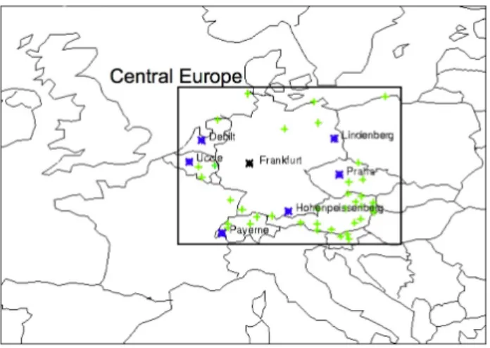
The main area of interest, referenced hereafter as “Central Europe”, is defined as the region between 44◦N and 55◦N latitude, and 3◦E and 18◦E longitude, which encompasses Frankfurt and several sounding stations. Figure 1 shows a map of this region and the measurement sites, where Frank-furt is denoted by a black star.
Six ozone sonde stations located near Frankfurt provided data over the period 1995–2008: Debilt, Hohenpeissenberg, Lindenberg, Payerne, Praha and Uccle (blue stars). The sounding data are available through the World Ozone and Ultraviolet Radiation Data Center (WOUDC, http://www. woudc.org). The ozone sonde data are treated as in Tilmes et al. (2011). The profiles already include the corrections performed by the data centers. For each profile a correction factor is suggested by the data center to scale the profile to ground-based ozone column measurements, for which the stratospheric fraction is dominant. This factor has not been applied here as it has little impact on the mean tropospheric profile, but we disregard profiles with a correction factor outside the range of 0.8 and 1.2. This filtering has only a small impact on the averaged profile between 1995 and 2009 (Tilmes et al., 2011). However, we filter out single profiles with column ozone values of more than 700 DU or of less than 50 DU, which would present unrealistic values of ozone profiles at the stratospheric maximum. The sonde profiles are binned the same way as MOZAIC profiles. For the elevated sites (Hohenpeissenberg and Payerne), the surface layer is 950–850 hPa instead of 1050–950 hPa.
More than 180 EMEP (European Monitoring and Eval-uation Program) surface stations provide measurements of ozone concentrations. However, we keep only the EMEP sta-tions located within our Central Europe region and having performed continuous measurements over the period 1998– 2008. The data from the 48 remaining sites are filtered to retain only morning measurements so as to avoid a high diur-nal variability and keep the same time window as the sondes. The surface stations appear as the green plus markers on the map (Fig. 1).
3 Methodology
As stated in the introduction, we aim to discuss and quan-tify the uncertainty associated with low sampling frequency measurements such as ozone sondes. The methodology
de-Fig. 1. Map of Europe. The Central Europe region, defined by the area between 44◦N and 55◦N latitude, and 3◦E and 18◦E longi-tude, is shown in the black rectangle. The MOZAIC city, Frankfurt, is shown with a black star, the six ozone sounding sites with blue stars and the EMEP surface stations with green plus symbols.
tailed below explains how we subsampled the high frequency MOZAIC data set of ozone profiles over Frankfurt to create subsamples with sampling frequency similar to those of the European ozone sonde data sets.
3.1 Time autocorrelation and effective sample size
Temporal autocorrelation in time series can significantly re-duce the amount of information that would be available from the same number of independent data points, and thus in-crease the error estimates. We have tested the temporal corre-lation in the MOZAIC daily time series of ozone profiles over Frankfurt. Ozone profiles over Frankfurt from the MOZAIC aircraft are numerous but not regular, leading to individual or several days within a month that are not documented. Miss-ing values in the daily time series of a month will have an effect on the estimation of autocorrelation. In order to avoid any misrepresentation of the temporal autocorrelation, we calculate time correlation based on months that have at least one profile a day. There are sixty-one months of the kind over the period 1995–2008. When more than one profile a day is available, the profile for this day is randomly selected. Sixty-one daily time series of one month are analyzed for each of the seven pressure layers. We estimate the first order autoregressive coefficient (r1) for each month and then take
the average of these estimates across the months. We found that the estimated autoregressive coefficient r1(between
ad-jacent days) is about 0.10–0.26 with a maximum value at 900 hPa and a minimum value at 600 hPa (Table 1). Using all the available months (168 = 12 · 14) to estimate r1leads
to a range of 0.17–0.35.
To test the significance level of r1, we use the one-sided
test recommend by WMO (1966) and compute the 95 % sig-nificance level for r1with
Table 1. First order autoregressive coefficients (r1) and scaling factors for effective sample size derived from the 61 full months at rate 1/1 (sample every day), rate 1/2 (sample every other day) and rate 1/4 (sample every fourth day).
Rate 1/1 Rate 1/2 Rate 1/4 Pressure level r1 f1/1=1−r1+r11 r1 f1/2= 1−r1 1+r1 r1 1000 hPa 0.15 0.74 0.03 0.94 0.08 900 hPa 0.26 0.59 0.17 0.71 0.03 800 hPa 0.21 0.65 0.14 0.75 0.02 700 hPa 0.14 0.75 0.09 0.83 0.03 600 hPa 0.10 0.82 0.05 0.90 0.05 500 hPa 0.11 0.81 0.00 1.00 0.05 400 hPa 0.13 0.77 0.03 0.94 0.08 300 hPa 0.16 0.73 0.03 0.94 0.04 r1,.95= −1 + 1.645 √ (Nd−2) Nd−1 (1) where Ndis the number of daily observations (i.e. 29 to 31).
For Nd=30, r1,.95=0.26. As a result, r1is below or at the
limit of the threshold, which means that the null hypothe-sis of no relationship between adjacent days (ρ1=0)
can-not be rejected. In other words, adjacent day observations may be uncorrelated, especially in the free troposphere above 800 hPa. We also determine the minimum time lag neces-sary to reach independence between observations by screen-ing the correlogram of each month. We estimate that inde-pendence is reached when the autocorrelation coefficient is lower than the 95 % confidence limit −N1
d +
2
√
Nd (equal to
0.30 for Nd=30). Using the 61 full months only, we found
that independency is reached for a time lag of one day in about 62–90 % of the cases and two days in another 7–31 % of the cases (the percentage depends on the pressure level). Less than 7 % of the correlograms show significant correla-tion for time lag equal to or higher than 3 days. These first results suggest that ozone measurements made every other day are generally independent. We further subsampled the 61 full months at two sampling rates: rate 1/2 (sample every other day) and rate 1/4 (sample every fourth day), creating 122 (61 · 2) time series at rate 1/2 and 244 (61 · 4) at rate 1/4. We estimate the first order autoregressive coefficient for each time series and take the average of these estimates across the time series. The results are reported in Table 1. The autocor-relation between observations made every other day is lower than 0.17, supporting an independence of observations made every other day. As expected, we found that the samples at rate 1/4 do not present significant temporal autocorrelation.
As the first order autoregressive coefficient is found to be significant for these Frankfurt daily time series of tropo-spheric ozone, the sample size needs to be adjusted for auto-correlation in time series. However, as previously stated, the MOZAIC measurements are irregular and this makes it diffi-cult to estimate r1for each month. As a result, we have used
the same average estimate r1 for all months. The effective
sample size for one month is given by
Nd,eff=Nd·f = Nd
1 − r1
1 + r1
. (2)
A first order correlation of 0.26 leads to a scaling to about 59 % of the original sample size. The scaling factors (f ) are given in Table 1 (f1/1for every day sample and f1/2for every
other day sample, for every fourth day sample we will con-sider f1/4=1). The effective sample size will be used to
es-timate the standard error and confidence interval on the sea-sonal means in Sects. 3.5 and 4 for Frankfurt and in Sect. 5 for the other northern midlatitude sites. We also estimate the proper scaling factors for Windhoek and use them in Sect. 6 (factors not shown).
3.2 Morning subset of the Frankfurt MOZAIC data set
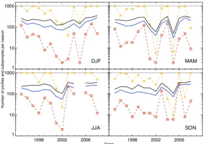
The methodology used in this paper aims to mimic the ozone sonde sampling. Sondes are launched generally at 11:30 UT or 12:00 UT in five of the six ozone sonde stations located in Central Europe (Debilt, Lindenberg, Payerne, Praha and Uccle) and around 05:30 UT at the Hohenpeissenberg sta-tion. To avoid the effect of a strong diurnal cycle in the lowest levels and to match the time window of the balloon launch in Central Europe, we retain the MOZAIC profiles taken between 05:00 and 13:00 UT. Figure 2 shows the num-ber of MOZAIC profiles (black line) per season for each year as well as the number of profiles per season available within this morning time window (blue line). As most of the MOZAIC flights were transatlantic, they took off and landed in the morning in Frankfurt. As a result, the morning sub-set of ozone profiles over Frankfurt represents 79 % of the entire dataset and often includes more than 100 profiles per season (Fig. 2). The morning subset of this data set includes on average more than one profile per day, allowing us to sub-sample each month at two typical sonde frequencies: 4 and 12 profiles a month (i.e. 12 and 36 profiles per season) as de-scribed hereafter. However, the reader should keep in mind that the profiles are taken irregularly, meaning that there are
Fig. 2. Time record of the number of vertical profiles taken per sea-son over Frankfurt between 1995 and 2008, in the whole data set (black) and in the morning (blue) subset in solid lines. The number of seasonal subsamples created with a frequency of 4 (orange) and 12 (red) profiles a month using the “regular” sampling method is shown by the dashed lines.
days with more than two profiles, days with one or two pro-files, and even days without observations.
3.3 Monthly subsampling
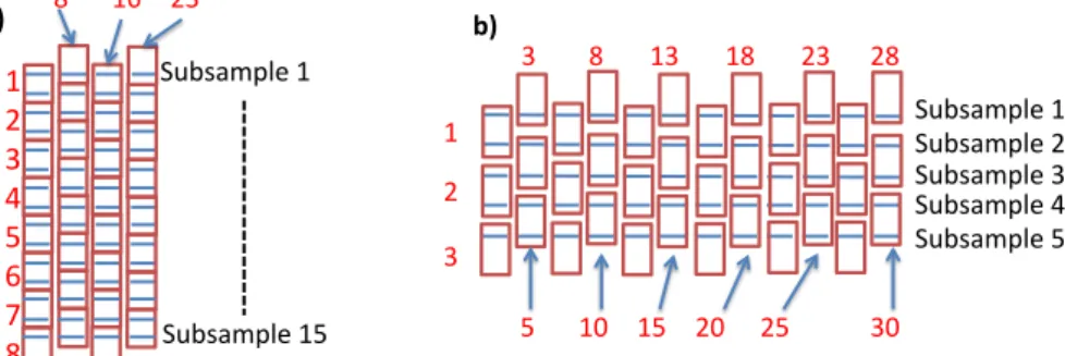
To better mimic the regular sampling of the soundings and to create subsamples, we use a “regular” sampling method, which is illustrated in Fig. 3. The subsampling is done for each month; this is why we consider two frequencies (Nf)
equal to 4 or 12 profiles per month. Consider a theoretical month documented with 60 regularly-spaced profiles (twice a day, which is close to the reality at Frankfurt). If we subsam-ple this data set to 4 profiles, we can create 60/4 = 15 sub-samples by taking every 15th profile. Considering there were two profiles a day, the first subsample corresponds to day 1 (1st profile), day 8 (2nd profile), day 16 (1st profile) and day 23 (2nd profile) (Fig. 3a), i.e. one profile every week. The second subsample corresponds to day 1 (2nd profile), day 9 (1st profile), day 16 (2nd profile) and day 24 (1st profile); and so on for the other subsamples. If we want subsamples of 12 profiles using the same month, then we create 60/12 = 5 subsamples by taking every 5th profile. As a result, the first subsample corresponds to one profile of days 1, 3, 6, 8, 11, 13, 16, 18, 21, 23, 26, 28; the second subsample corresponds to one profile of days 1, 4, 6, 9, 11, 14, 16, 19, 21, 24, 26, 29; the third subsample corresponds to one profile of days 2, 4, 7, 9, 12, 14, 17, 19, 22, 24, 27, 29; and so on (Fig. 3b). In this example, we take a profile every 2 or 3 days, which is close to the reality of the thrice-weekly sampling of soundings. In the case of a number of profiles a month which is not divisi-ble by 4 or 12, some profiles are not used as we do not allow multiple uses of profiles.
This method avoids selecting sequential days, which is consistent with the sampling frequency of ozone sondes, even though some MOZAIC profiles are discarded in this way. Except for a few months which are documented with fewer than 40 profiles, we were able to create more than 10 subsamples of 4 profiles. On the contrary, there were less than 10 subsamples created with 12 profiles for each month because there are fewer than 120 profiles per month. As a compromise between representativity and data availability, we limit the number of monthly subsamples to 10 for both frequencies. As a consequence, for the example of 60 profiles we would use only the first 10 subsamples of 4 profiles. The reader should note here that the irregularity of the MOZAIC measurements makes it difficult to sample exactly every 2 or 3 days (or every week) as presented in the example in Fig. 3. The sampling chosen here leads to slightly different sampling days than those of the ozone sondes. However, considering the high number of profiles over Frankfurt (except in 2002 and 2005), the sampling frequencies are similar (weekly or thrice weekly) to those of the ozone sonde frequencies and allows to produce more samples.
We also tried a “random” sampling method in which the profiles are randomly picked within the month. A random sampling allows eventually to consider any profiles and to create 10 subsamples, whatever the number of profiles avail-able and their frequency. Despite the fact that profiles from sequential days might be selected, potentially giving more weight to a particular time/event in the monthly mean, this method provides similar results.
3.4 Creation of the seasonal subsamples
The seasonal subsamples are derived from the monthly sub-samples. If there are n1, n2 and n3 subsamples for month 1, month 2 and month 3 respectively, then we derive nNf
seas,yr=
n1 × n2 × n3 subsamples for a given season and year. Conse-quently, a monthly subsample may be used in several sea-sonal subsamples. The number of subsamples created per season and per year is given in Fig. 2. As there are up to 10 monthly subsamples, the maximum number of seasonal subsamples is 1000. This value is often reached for the fre-quency of 4 profiles a month. On the contrary, since gener-ally less than 10 monthly subsamples of 12 profiles could be created, the maximum of seasonal subsamples at this fre-quency is around 120. Using this “regular” sampling method, the number of subsamples is highly dependent on the number of profiles available. In particular, fewer profiles were avail-able for the years 2002 and 2005, especially in the spring and summer (Fig. 2). In order to keep a minimum of two subsam-ples per season, per year and for each frequency, we discard the spring of 2005 and the summers of 2002 and 2005 from our discussion. Discarding these years does not significantly affect the results regarding the trends presented in Sect. 4.4.
Subsample*1* Subsample*2* Subsample*3* Subsample*4* Subsample*5* 1* 2* 3* 3********8*******13*******18*******23******28******** 5 *10 *15 *20 **25 * *30 ** Subsample*1* Subsample*15* 1* 2* 3* 4* 5* 6* 7* 8* 8 *16 *23* a)# b)#
Fig. 3. Illustration of the “regular” sampling method based on a theoretical month, for which 60 profiles are available (shown as small blue lines). We consider here that two profiles per day are available. Each day is represented as a red box and the red number is the day of the month from 1 to 30. In (a) we can create 15 (60 divided by 4) subsamples of four profiles each. The first subsample corresponds to day 1 (1st profile), day 8 (2nd profile), day 16 (1st profile) and day 23 (2nd profile). In (a), day 8 is repeated in the second column to include two profiles (same for day 23). The second subsample corresponds to day 1 (2nd profile), day 9 (1st profile), day 16 (2nd profile) and day 24 (1st profile); and so on for the other subsamples. In (b) we create 5 (60 divided by 12) subsamples of 12 profiles each. The first subsample corresponds to one profile of days 1, 3, 6, 8, 11, 13, 16, 18, 21, 23, 26, 28. Days 3, 8, 13, 18, 23 and 28 are repeated from the bottom of a column to the top of the next column. This method allows the selection of regularly spaced profiles.
3.5 Definition of the metrics
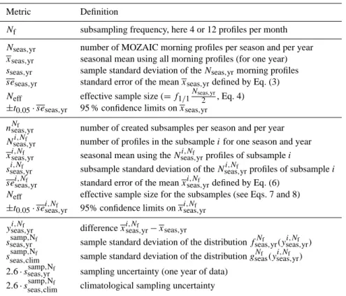
In this study, we aim to give a quantitative estimate of the uncertainty that arises from low time resolution, depending on the season, altitude level and sampling frequency. We ex-plain here how we define the sampling uncertainty and other metrics presented in the text and figures. A summary of the metrics is presented in Table 2.
3.5.1 Seasonal mean, standard error and confidence limit
First, we calculate the seasonal mean concentrations of ozone at each pressure level. For each year, we define by xseas,yrthe
seasonal mean derived from the Nseas,yr MOZAIC morning
profiles; the subscript “seas,yr” means that this value is de-rived for each season and year. The sample standard devia-tion associated with the seasonal sample of Nseas,yrprofiles
is called sseas,yr. The standard error of the mean xseas,yr is
defined by seseas,yr= sseas,yr √ Neff (3) with Neff=f1/1 Nseas,yr 2 (4)
Neff is the effective sample size accounting for
autocorrela-tion in the daily observaautocorrela-tions. The scaling factor f1/1is that
derived in Sect. 3.1. However, there are on average two pro-files per day in the Frankfurt morning data set. Assuming that a second profile taken the same day does not provide more information than the first one, we divide Nseas,yrby 2. Using
an effective sample size instead of the real size of the sample
increases the standard error estimate. The seasonal distribu-tions of the MOZAIC measurements are found to be close to normal except for the lowest levels, for which the distribu-tions are cut off at zero due to ozone titration by NO in the vicinity of the airport. In these cases, part of the theoretical normal distribution would be in the negative side, which is not realistic for ozone concentrations. The 95 % confidence interval for xseas,yris defined as
CI95 %= [xseas,yr−t0.05·seseas,yr, xseas,yr+t0.05·seseas,yr] (5)
where t0.05 is the 95th percentile of the Student’s
t-distribution with Neff−1 degree of freedom. This confidence
interval is represented in Fig. 4 by the blue vertical error bars. For the lowest levels where the distributions are skewed, the confidence interval may not represent a 95 % confidence in-terval, however, for clarity, we keep the same metrics for the lowest levels.
Similar definitions are used for a subsample of the MOZAIC morning data set. Considering there are Ni,Nf
seas,yr
profiles in a subsample i, whose seasonal mean is xi,Nf
seas,yr,
then the standard error of the mean is defined as
sei,Nf seas,yr= si,Nf seas,yr √ Neff (6) where si,Nf
seas,yris the sample standard deviation of the
subsam-ple i and with
Neff=f1/2Nseas,yri,Nf for Nf=12, and (7)
Table 2. List of the metrics used and their definition. t0.05 is the 95th percentile of the Student’s t-distribution with Neff−1 degrees of freedom. Neffis defined in Eq. (4) for the morning data set and in Eqs. (7) and (8) for the subsamples.
Metric Definition
Nf subsampling frequency, here 4 or 12 profiles per month Nseas,yr number of MOZAIC morning profiles per season and per year
xseas,yr seasonal mean using all morning profiles (for one year)
sseas,yr sample standard deviation of the Nseas,yrmorning profiles seseas,yr standard error of the mean xseas,yrdefined by Eq. (3) Neff effective sample size (= f1/1
Nseas,yr
2 , Eq. 4) ±t0.05·seseas,yr 95 % confidence limits on xseas,yr
nNf
seas,yr number of created subsamples per season and per year Nseas,yri,Nf number of profiles in the subsample i for one season and year xi,Nf
seas,yr seasonal mean using the Nseas,yri,Nf profiles of subsample i si,Nf
seas,yr subsample standard deviation of the Nseas,yri,Nf profiles of subsample i sei,Nf
seas,yr standard error of the mean xi,Nseas,yrf defined by Eq. (6) Neff effective sample size for the subsamples (see Eqs. 7 and 8) ±t0.05·sei,Nseas,yrf 95% confidence limits on xi,Nseas,yrf
yi,Nf
seas,yr difference xi,Nseas,yrf −xseas,yr ssamp,Nf
seas,yr sample standard deviation of the distribution fseas,yrNf (yseas,yri,Nf ) sseas,climsamp,Nf sample standard deviation of the distribution gNf
seas(yi,Nseas,yrf )
2.6 · ssamp,Nf
seas,yr sampling uncertainty (one year of data)
2.6 · ssamp,Nf
seas,clim climatological sampling uncertainty
Here the superscript “i, Nf” denotes reference to a subsample
iat the frequency Nf. The number of profiles Nseas,yri,Nf per
sea-son and per year is equal to 12 or 36 for a frequency Nf=4 or
12 respectively. For a frequency of Nf=12, which leads to a
sampling every other day or every three days on average, we use the first order autoregressive coefficient derived for the rate 1/2 in Sect. 3.1 as an estimate of the autocorrelation in the monthly subsamples. Thus the subsample size (Ni,Nf
seas,yr)
is scaled with the factor f1/2. For the frequency Nf=4, the
results found in Sect. 3.1 suggest insignificant autocorrela-tion between profiles taken every week. Thus we use the real subsample size to estimate the standard error. The confidence interval for each of the subsample means is calculated as CI95 %=t0.05·sei,Nseas,yrf (9)
where t0.05 is the 95th percentile of the Student’s
t-distribution with Neff−1 degree of freedom. 3.5.2 Sampling uncertainty
In order to assess the effect of low sampling frequency, we analyze the differences between the overall seasonal mean
xseas,yr, derived from the morning MOZAIC data set,
defin-ing our true value, and the biased seasonal means derived from the generated low frequency subsamples xi,Nf
seas,yr(i = 1,
nNf
seas,yr with nNseas,yrf the number of subsamples of 4 or 12
profiles a month created for a given season and year). We note yi,Nf
seas,yr=xi,Nseas,yrf −xseas,yr these differences. At a
fre-quency Nf=4, there are generally nNseas,yrf =1000
subsam-ples per season and per year, while at the frequency Nf=12,
nNf
seas,yr is lower than 120 and around 50–70 (Fig. 2). For
each year and each season, we consider the discrete proba-bility distribution of these differences fNf
seas,yr(yseas,yri,Nf )
com-posed of nNf
seas,yrsubsamples. The sample standard deviation
associated with the distribution fNf
seas,yris called sseas,yrsamp,Nf, the
superscript “samp” referring to “sampling uncertainty” and the subscript “seas,yr” recalling that this value is derived for a given year and season. The number of seasonal sub-samples in each year is generally large enough to make the distributions fNf
seas,yr close to normal. This is true for a
fre-quency of Nf=4, but less frequent at Nf=12, especially for
particular years such as 2002, 2003 or 2005, when nNf
seas,yr
is below a few dozens (Fig. 2). We defined, for each year and each season, the sampling uncertainty on the observed means as 2.6 · ssamp,Nf
seas,yr . In the case of a normal distribution,
this value corresponds to the 99 % sampling uncertainty and ensures that 99 % of the biased seasonal means are within
±2.6·ssamp,Nf
seas,yr . When the number of subsamples is below this
limit, we keep the same estimate; even though it does not cor-respond to 99 % of the probability distribution, it still gives a range for the biased seasonal mean spread.
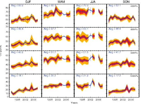
Fig. 4. Time evolution of the ozone seasonal means over Frankfurt between 1995 and 2008 as observed by MOZAIC aircraft at four pressure levels (1000, 800, 600, 400 hPa, from bottom to top). The seasonal mean (xseas,yr) from the morning data set is shown in blue with the 95 %
confidence limit error bars (CI95 %=t0.05·seseas,yr). The shaded areas represent the sampling uncertainty (range [xseas,yr−2.6 · sseas,yrsamp,Nf, xseas,yr+2.6 · sseas,yrsamp,Nf], see Sect. 3.5.2 for details) derived from the ensemble of subsamples of 4 (orange) and 12 (red) profiles a month for
each year and season. At the top left corner of each rectangle, the average seasonal means over the entire period are shown.
In order to obtain a single value per season (and per alti-tude level), we aggregated the 14 distributions fNf
seas,yr from
each year in the period 1995–2008 into a single distribution, which we call gNf
seas. For each season, the resulting
distribu-tion gNf
seas(yseas,yri,Nf )is then composed of approximately 9000
(800) seasonal subsamples for a frequency of Nf=4 (12)
profiles a month. These distributions are found to be nor-mal and are fitted with a gaussian distribution. We call sam-pling uncertainty the value given by 2.6 · ssamp,Nf
seas,clim(the
sub-script “clim” refers here to “climatology”), where ssamp,Nf
seas,clim
is the sample standard deviation of the fitted distribution. We consider the fitted standard deviation of the distribution in order to exclude outliers, which appear mainly in win-ter and spring. The fitted sample standard deviation is sim-ilar to the sample standard deviation for distributions free of outlier. This sampling uncertainty estimate ensures that 99 % of the seasonal means derived from the subsamples are within ±2.6 · ssamp,Nf
seas,climof their true value. This time, s samp,Nf
seas,clim
refers to a seasonal estimate derived using the whole morn-ing MOZAIC period, and we have called it climatological sampling uncertainty.
4 Effect of the sampling over Frankfurt
In this section, we discuss to what extent the sampling im-pacts on the observed seasonal means and the annual and inter annual variabilities using the ensemble of subsamples created from MOZAIC morning profiles over Frankfurt.
4.1 Sampling uncertainty on the ozone seasonal mean
Figure 4 presents the variations of ozone concentrations from the MOZAIC morning subset over Frankfurt (in blue) be-tween 1995 and 2008 at four pressure levels (1000, 800, 600 and 400 hPa) and for the four seasons (winter, spring, sum-mer and fall). The error bars on the seasonal means are shown in blue in Fig. 4 and correspond to the 95 % confidence lim-its, CI95 %calculated from Eq. (5).
The shaded areas represent the 95 % sampling uncertainty (range of the biased seasonal means, defined as ±2.6·ssamp,Nf
seas,yr
in Sect. 3.5.2) at the two frequencies Nf=4 and 12 (in
or-ange and red respectively). As expected, the sampling un-certainty on the seasonal mean increases when the sampling frequency decreases. The results show that the sampling un-certainty is larger than the 95 % confidence limit on the“true” seasonal mean, especially for the lower frequency Nf=4.
We use the climatological sampling uncertainty (2.6 ·
ssamp,Nf
seas,climdefined in Sect. 3.5.2) to draw a more general
pic-ture of the results for each season. Table 2 summarizes the values of these climatological sampling uncertainties in per-centages relative to the true value of the seasonal mean for four pressure levels. In addition, Fig. 5 shows the vertical profiles of the climatological sampling uncertainty in orange and red solid lines for the frequencies Nf=4 and 12
respec-tively. The sampling uncertainty on the seasonal mean ranges between 9 to 29 % for the 4 profile-a-month data sets as com-pared to 5–15 % for the 12 profile-a-month data sets. For sur-face ozone, the narrowest ranges in ppb are observed in the winter and fall. However as these months have lower ozone concentrations, the uncertainty on the seasonal mean repre-sents up to 15 and 29 % of the true value for a frequency of 4 and 12 profiles a month respectively. In the free tropo-sphere, the lowest uncertainty is found in winter. The sam-pling uncertainty on the seasonal mean, as calculated in our study, is higher than 10 % at the lowest time resolution, ex-cept between 700 and 500 hPa for most of the seasons. For a 12 profile-a-month frequency, the sampling uncertainty gen-erally drops below 10 % in the free troposphere. The lowest sampling uncertainty is observed in the free troposphere at 700 hPa. This result suggests that over Frankfurt the 700 hPa level is the best candidate for comparing observations to other observations or to models and limiting the bias due to different sampling frequencies. At this level, the sampling uncertainty is 4.6, 4.2, 5.5, 5.6 % for winter, spring, summer and fall respectively for a 12 profile-a-month dataset (8.6, 9.0, 10.8, 8.7 % for 4 profile-a-month).
The sampling uncertainty on the seasonal means derived from the “random” sampling method is generally similar but slightly higher than the values derived from the “regular” sampling method (not shown). The estimates of the sampling uncertainty from this method are generally within 4 age points (unit of an arithmetic difference of two percent-ages) of the values presented for the “regular” method in Ta-ble 3, with exceptions in the lowest levels where the differ-ences may reach 17 percentage points.
In Fig. 5 we also compare the sample standard deviation at different frequencies. For the entire morning data set, the sample standard deviation (sseas,yr) is estimated for each year
(for each season and pressure level) and we plot the average of these estimates across the years in dot-dashed blue line. For the frequency Nf=4 or 12, the sample standard
devia-tion (si,Nf
seas,yr) is estimated for each subsample and each year
(for each season and pressure level), and we plot the average of these estimates across the subsamples and the years in a dot-dashed orange or red lines. The results show that the av-erage sample standard deviation is similar whatever the sam-pling frequency, although a bit higher when considering the high frequency data set. Also, the sample standard deviation is always higher than the sampling uncertainty on the sea-sonal means. Both metrics (sample standard deviation and
Fig. 5. Vertical profiles of the climatological sampling uncertainty (2.6 · ssamp,Nf
seas,clim, see Sect. 3.5.2) derived from Frankfurt MOZAIC
data for the four seasons (orange and red solid lines for the fre-quency of Nf=4 and 12, respectively). The blue dot-dashed line
represents the average value of the sample standard deviation
sseas,yr derived from the whole morning data set (average across
years for each season and level), and the orange and red dot-dashed line the average values of the sample standard deviation si,Nf
seas,yr
de-rived from the subsamples (average across years and across sub-samples for each season, level and frequency). Similarly, the dashed lines represents the average estimate of the 95 % confidence limits on the seasonal means (t0.05·seseas,yrin blue and t0.05·sei,Nseas,yrf in
orange and red). The black solid line shows the profiles of ozone in-ter annual variability as calculated in Sect. 4.2. The vertical dotted lines are the 5 and 10 % value lines, uncertainty values commonly quoted for measurement error of ozone sondes.
sampling uncertainty) have a well-marked C-shape, show-ing higher variability of ozone concentrations in the bound-ary layer (air masses affected by fresh emissions, subject to dry deposition of ozone, turbulence) and in the upper tro-posphere (potential impact of stratosphere-trotro-posphere ex-changes). Higher variability between the profiles enhances the potential differences between subsamples and then makes the distributions fNf
seas,yr(yseas,yri,Nf )broader at these levels
com-pared to those in the middle troposphere.
Assessment of the sampling uncertainty for any site re-quires high frequency data set, which is not feasible. In the following we suggest an easy-to-calculate estimate of the sampling uncertainty suitable for any tropospheric ozone data set. As presented in the Methodology, the 95 % confi-dence limit on the seasonal mean has been calculated for the MOZAIC morning data set as well as for any subsam-ple, this confidence interval being easy to calculate. We take the average of these values across the subsamples and across the years to derive an estimate of the mean 95 % confidence limit on the seasonal mean for both frequencies. These esti-mates are plotted as orange and red dashed lines in Fig. 5. The results show that the average 95 % confidence limit on
the biased seasonal mean is close to the sampling uncertainty we derived in this study (an absolute difference of less than 3 percentage points). This also means that the 95 % confi-dence interval (as defined in this study) of the seasonal mean produced by the subsample most probably contains the true mean value. As expected, this average 95 % confidence limit on the seasonal mean using the entire morning data set of profiles (blue dashed line) is much lower than the confidence limit using fewer profiles.
4.2 Sampling effect on observed annual and inter-annual variabilities
Our results show that different low time frequency samples may show substantially different seasonal means and suggest that the derived annual and inter annual variabilities may be biased by the sampling.
In Fig. 4, we observe that the seasonal cycle is well marked in the entire morning data set. The seasonal differences of the long-term means between the cold and the warm months (DJF vs. JJA) are 41, 33, 28 and 72 % of the cold month con-centrations (22 to 42 % of the warm months), respectively for the four pressure levels considered (from the top to the sur-face, see Fig. 4). These differences are higher than the sam-pling uncertainty on the seasonal means (Table 3), meaning that the seasonal cycle can be distinguished even when using the low frequency measurements.
The variability of ozone concentrations from one year to another (for each season) is calculated from the morning MOZAIC subset as (xseas,yr+1−xseas,yr)/xseas,yr. On
aver-age, over the four seasons, the inter-annual variability (IAV) is below 8 % in the free troposphere and ranges between 7 and 20 % in the two lowest levels (black solid lines in Fig. 5). As a result, the observed IAV signal is generally higher than the 95 % confidence limit of the seasonal means derived from the MOZAIC morning data set (dashed blue line), except at the highest altitude levels. This suggests that a high fre-quency data set may be used to disclose inter-annual vari-ability in the tropospheric ozone. When using a data set at a frequency of 12 profiles a month, this capacity is reduced. For the frequency Nf=4, the sampling uncertainty is much
higher than the inter-annual variability, leading to an uncer-tain IAV in such low frequency data sets. Consequently, ex-cept for extreme events, the IAV signal might possibly be masked by the sampling effect and the observed IAV signal will be highly dependent on the sampling, especially at the lowest time resolution over this region.
4.3 Sampling uncertainty versus measurement uncertainties
First, it is worth noting that the MOZAIC instrument un-certainty is typically 2–3 ppb for a concentration lower than 50 ppb (5 %), which is lower than the sampling uncertainty on the seasonal mean.
The accuracy of ozone sonde measurements is often quoted as ±5 % (Smit and Kley, 1998). A series of experi-ments evaluated the sonde performance and indicated a pre-cision of better than ±(3–5) % and an accuracy of about ±(5– 10) % up to 30 km altitude if standard operating procedures for ECC sondes are used (Smit et al., 2007). These values are represented on Fig. 5 in dotted lines. The sampling uncer-tainty as estimated in our study is always higher than 5 % ac-curacy. Between 900 and 400 hPa, the sampling uncertainty at the frequency of Nf=12 is within the accuracy range of
5–10 %. At a frequency of Nf=4, the sampling uncertainty
is generally higher than 10 %, except around 700 hPa.
4.4 Sampling effect on ozone trends
To assess the effect of sampling frequency on ozone trends, we calculated the linear trend over the period 1998–2008. This time period is shorter than the MOZAIC period, but corresponds to a period over which the sonde and MOZAIC measurements agree the best (Logan et al., 2012; Tilmes et al., 2011). Seasonal ozone trends over the period 1998– 2008 are derived from the whole morning MOZAIC data set using a weighted linear regression. For each seasonal mean, the standard error on the mean (seseas,yr) is used as an error
measurement in the linear regression; the weight put on a sea-sonal mean is then the inverse of the square root of the stan-dard error. Using the same approach, linear trends are also derived from the measurements made at the six European sonde sites and the 48 EMEP surface stations. Weighting the seasonal means with the standard error allows us to take into account the uncertainty for each of them. The weight-ing greatly raises the uncertainty estimate of the trend, but the trend magnitude remains unchanged. As a consequence, the 1-sigma uncertainty of the trend is highly dependent on the standard error of the mean seseas,yrused for the
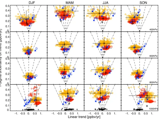
weight-ing, and therefore dependent on the number of data. Figure 6 displays the distribution of the trends and the 1-sigma un-certainty estimates of these trends for the whole morning MOZAIC data set (black diamond), the European sondes (blue stars) and the surface station (black plus). In order to visualize the significance of the trend, the dashed lines cor-responding to y = x and y = x/2 (i.e. 1-sigma = slope and 2-sigma = slope) are added; this means that markers falling between the dashed lines represent trends that are not statis-tically significant.
The MOZAIC morning subset shows positive trends in winter and fall in the lowest level, while the surface ozone trend in summer is negative (−0.3 ppbv yr−1). The trends
derived using all MOZAIC profiles (and not only morn-ing profiles) show a negative summer trend of around
−0.7 ppbv yr−1. These results for surface ozone are in agree-ment with previous studies (Ord´o˜nez et al., 2005; Zbinden et al., 2006; Jonson et al., 2006; Oltmans et al., 2006; Jean-net et al., 2007; Gilge et al., 2010). They most probably re-sult from the decrease in ozone precursor emissions during
Linear trend [ppbv/yr]
1-Sigma uncertainty on trend [ppbv/yr]
-1. -0.5 0. 0.5 1. 0. 0.1 0.2 0.3 0.4 0.5 DJF D U PrPa L H MAM D U Pr L PaH JJA D U L Pa H 400hPa SON D U L Pa H 0. 0.1 0.2 0.3 0.4 0.5 D U Pr L Pa H D U Pr L PaH DL U Pa H 600hPa D U L PaH 0. 0.1 0.2 0.3 0.4 0.5 D UPr L PaH D UPr L Pa H D U L Pa H 800hPa D U L Pa H -1. -0.5 0. 0.5 1. 0. 0.1 0.2 0.3 0.4 0.5 D UPr L PaH -1. -0.5 0. 0.5 1. D UPrL Pa H -1. -0.5 0. 0.5 1. D UL Pa H -1. -0.5 0. 0.5 1. 1000hPa D U L PaH
Fig. 6. 1-sigma uncertainty estimate of the linear trend against the linear trend for the four seasons and at four pressure levels (1000, 800, 600, 400 hPa, from bottom to top). Black plus symbols give the trends at 48 surface stations. The linear trend is calculated over the period 1998–2008. Blue stars show the trends derived from ozone sondes at the six stations (D = Debilt, H = Hohenpeissenberg, L = Lindenberg, Pa = Payerne, Pr = Praha, U = Uccle) at 1000 hPa except for H and Pa, value at 900h Pa. The black diamond corresponds to the trends derived from the whole morning MOZAIC data set in Frankfurt. For each frequency, 200 random time series were created from the ensemble of Frankfurt subsamples. The resulting trends are given by the cloud of diamonds in red (frequency of 12 profiles a month) and orange (4 profiles a month). The mean, minimum and maximum of these distributions are shown with the vertical and horizontal black thin lines. The dashed and dot-dashed lines show the 67 % and 95 % confidence limit lines for the slope.
this period. In the cold months, the trend probably results from a reduced ozone titration by nitrogen monoxide. Dur-ing summer, the decrease in ozone precursors probably leads to a weaker photo-chemical ozone production during pollu-tion episodes. Surface stapollu-tions give the lowest uncertainty in the slope due to their large amount of data. Most suggest a positive trend in winter and spring, whereas in summer and fall, trends appear more scattered around zero. The sea-sonal trends vary with the altitude of the stations (not shown). Above 1 km, the results suggest a negative trend in summer, positive in winter and spring, and a near-zero trend during the fall season, in agreement with MOZAIC measurements in Frankfurt. Trends derived from the sondes are also scat-tered around zero, in a range similar to the surface stations. Local effects in the boundary layer prevent us from draw-ing any conclusions without proper analysis of the vicinity of each site (which is beyond the scope of this study). However, this result highlights the range of the surface ozone trend in Europe.
In the free troposphere at 600 hPa, the seasonal trends de-rived from MOZAIC are weaker, and not always statistically significant, with negative trends in fall and spring and
posi-tive trends in summer and winter. These results are in agree-ment with the recent study of Logan et al. (2012). For the sondes (blue stars), as the number of profiles is lower, the un-certainty in the estimate of the trend is larger, leading gener-ally to insignificant trends. Some sonde measurements are in general agreement (same sign) with MOZAIC (e.g. Linden-berg, HohenpeisenLinden-berg, Payerne) while others are not (e.g. Debilt and Uccle in the free troposphere). Other studies have already highlighted such discrepancies between European sites (Oltmans et al., 2006; Logan et al., 2012), and Logan et al. (2012) suggest that unusually high or low ozone con-centrations measured at these sites in some years are respon-sible for these differences. In the upper level, the trends are more scattered around zero, except in fall when all present a negative trend (although of little significance for most of the sonde sites).
However, we have showed in the previous section that the observed seasonal means may be significantly impacted by the sampling frequency, especially at a frequency of Nf=4.
Thus there could be a potential effect of sampling on the ob-served ozone trend. To quantify this potential effect, we have created 200 random time series at each frequency (Nf=4
or 12). Each time series is built as follows: for each of the 11 yr, a seasonal subsample is randomly selected among the
nNf
seas,yravailable subsamples. As a result, we calculate an
en-semble of 200 linear trends for each sampling frequency. The linear trends are calculated in the same manner as described above for the MOZAIC morning data set. These 200 low fre-quency MOZAIC trends are over-plotted in Fig. 6 in red and orange diamonds for the 12 and 4 profile-a-month frequen-cies, respectively. The mean, maximum and minimum val-ues of these ensemble of trends and their estimates are rep-resented by the thin black lines over the cloud of points. The mean values of the trends derived from the ensembles are generally similar to the trends derived from the full MOZAIC morning subset (black diamond) (within 0.2 ppbv yr−1). As
expected, the scattering of the trends is greater at a frequency of 4 profiles a month than at 12 profiles a month. Winter and fall trends from the MOZAIC morning subset being well pronounced in the lowest level, the distribution of the sub-sample trends remains mainly in the positive quadrant. The narrowest scattering in the cold months is due to the lower variability of ozone (see Sect. 4.1). In summer and spring, the higher variability and the less marked trends result in a larger scattering around a null trend. Comparing the sonde trends (blue stars) to the Frankfurt subsample trends (clouds of red and orange diamonds), we observe that the uncertainty estimate of the trend of a given sounding station is close to that of the ensemble at a similar sampling frequency. Obvi-ously, this results from the measurement frequency at each station (close to 4–7 profiles a month for Debilt, Lindenberg and Praha and around 12 a month over Hohenpeissenberg, Payerne and Uccle). Also, the sonde trend markers fall sur-prisingly well within the red and orange clouds of Frankfurt subsamples, except for winter near the surface. If we consider the free troposphere only (altitude above 800 hPa), our results show that the linear trend derived from a subsample of Frank-furt data set could yield a value similar to those derived from any of the sondes, either positive or negative, in agreement or not with the MOZAIC morning data set. The trends extracted from low frequency data sets over the 1998–2008 period can be highly biased and not representative even if apparently significative. Thus our study suggests that the apparent afore-mentioned discrepancies observed between sondes, as well as between sondes and MOZAIC, may be attributed to sam-pling frequency, even though geophysical variations or dif-ferences in measurement strategy cannot be ruled out. How-ever, it is worth noting that our results apply for this specific time period (1998–2008), which presents small variations of ozone concentrations. We applied the same approach using the subsamples created with the “random” sampling method. The main characteristics of the distributions of trends ob-tained from the 200 random time series are generally similar to those using the “regular” sampling method (not shown).
5 Generalization to the Northern Hemisphere midlatitudes
In this section, we aim to generalize our results to the North-ern Hemisphere midlatitudes. The Frankfurt data set was the best candidate to start this study, since more than two profiles per day were collected. However, other cities in the North-ern Hemisphere are well documented, such as Vienna, Paris, New York, Boston, Tokyo and Osaka. The number of pro-files collected per season over these cities is summarized in Table 4.
For Frankfurt, Vienna, Paris and New York, the average number of profiles collected per season and per year allows subsampling these data sets at the two typical ozone sonde frequencies (more than 60 profiles per season on average). The data sets over Boston, Tokyo and Osaka have a lower frequency and thus can be subsampled only at the 4 profile-a-month frequency. In this section, all the profiles are kept without time filtering to retain the greatest number of pro-files. A test performed for Frankfurt shows that the time fil-tering affects only the lowest levels and has little influence in the free troposphere (not shown). Also, we use the “random” sampling method in order to produce the maximum num-ber of subsamples. The choice of sampling method reveals no significant impact on the results obtained for Frankfurt in Sect. 4; therefore we argue that applying this method here is appropriate. We use the same methodology as for the Frank-furt morning data set. We assume similar autocorrelation and use the ratio derived in Sect. 3.1 to calculate the effective sample size for the seven cities.
For these seven cities, we derive estimates of the clima-tological sampling uncertainty (defined as 2.6 · ssamp,Nf
seas,clim in
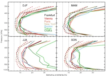
Sect. 3.5.2) in the same way as for the Frankfurt morning data set and then plotted these values against pressure lev-els in Fig. 7, color coded by cities. The vertical profiles for Vienna, Paris, New York and Boston are similar to those for Frankfurt in regards to the shape and the order of magnitude. As expected, the sampling uncertainty is higher at the low-est frequency for all these sites. They all show that the sam-pling uncertainty at a 12 profile-a-month frequency is lower than the 10 % measurement accuracy in the free troposphere (around 8 % between 500 and 800 hPa), while the sampling uncertainty at 4 profile-a-month frequency is systematically greater than the measurement accuracy of 10 %. For a fre-quency of 4 profiles a month, the sampling uncertainty is around 10–18 % between 500 and 800 hPa. These results also suggest a greater sampling uncertainty for Tokyo and Osaka (20 to 30 % in JJA and SON) than for Europe and North America in the summer and fall. This is in agreement with larger ozone distributions observed over the sonde stations at Tateno and Kagoshima in Japan for the same seasons (Tilmes et al., 2011). In addition, the mean sample standard devia-tion (average across subsamples and years) is much higher in summer and fall at the two Japanese sites than for the other five MOZAIC sites, which present a standard deviation
Table 3. Climatological sampling uncertainty, defined as the 2.6 ·
sseas,climsamp,Nf (see Sect. 3.5.2 for details). Values are given for the “regu-lar” sampling method in percentages relative to the overall seasonal mean at both sampling frequencies (Nf=4 or 12 profiles a month)
and at four pressure levels.
Frequency Nf Winter Spring Summer Fall
400 hPa 4 15.4 16.4 14.2 12.6 12 8.6 9.0 7.5 7.2 600 hPa 4 8.6 9.6 11.1 10.1 12 4.7 5.4 5.7 5.5 800 hPa 4 10.0 10.8 15.3 12.1 12 5.0 4.9 6.6 7.4 1000 hPa 4 29.2 23.6 24.9 27.5 12 15.0 11.7 12.9 10.3
similar in magnitude to that of Frankfurt (not shown). This Japanese region is influenced either by the pollution emitted by biomass burning in Siberia and China (Streets et al., 2003) or by poor ozone air masses transported from the tropics (Lo-gan, 1985). Moreover, there are large latitudinal gradients in ozone over Japan in the summer and autumn (Logan, 1999), so that ozone concentrations measured by the aircraft depend on their routes into and out of these airports. As a result, the variability sampled by the aircraft over Japan depends on the dynamic regime under which the site is at the time of the sampling (influence of monsoon circulation and con-vective systems, transport of midlatitude air masses). This leads to a greater variability of ozone concentrations in the Japanese free troposphere which largely impacts the distri-butions gNf
seas(yseas,yri,Nf ). Our results might also be biased by
the smaller number of profiles available for the two Japanese sites as compared to the North American and European sites. However, the results found for Boston, similar to Frankfurt even though even fewer profiles were available, tend to cor-roborate our findings for Tokyo and Osaka.
We also compared the vertical profiles of the average sam-pling uncertainty (2.6 · ssamp,Nf
seas,clim) with the vertical profiles
of the average 95 % confidence limit on the seasonal mean (CI95 %) for each of these cities (as in Fig. 5). For the sake of
clarity, we do not show these profiles in Fig. 7. As found for Frankfurt in Sect. 4.3, the sampling uncertainty for both fre-quencies is higher or similar to the 95 % confidence interval on the biased seasonal mean for all stations in the Northern Hemisphere (difference of 1–3 percentage points on average between 800 and 500 hPa). The 95 % confidence interval on the biased seasonal mean could be used as an estimate of the sampling uncertainty, although it may underestimate the sampling uncertainty slightly.
To conclude this section, the results derived from the de-tailed study undertaken for Frankfurt in Sect. 4 can be ex-tended to other northern midlatitude sites in Europe and
Fig. 7. Vertical profiles of the climatological sampling uncertainty in percentages (2.6 · ssamp,Nf
seas,clim) for the seven northern mid-latitude
sites, color-coded by cities. The sampling uncertainty at the fre-quency Nf=4 (12) is shown in solid (dashed) lines. As stated in the text, only Frankfurt, Vienna, Paris and New York are shown for the frequency Nf=12. The vertical dotted lines are the 5 and 10 %
value lines, uncertainty values commonly quoted for measurement error of ozone sondes.
North America, which are not influenced by strong changes in air mass composition (such as tropical air masses). For sites more similar to Tokyo and Osaka in terms of ozone variability, the sampling uncertainty is much higher during the summer and fall seasons. As a consequence, we suggest a careful interpretation of the observed ozone means (and ozone variations) over Japan.
6 Tropical case: Windhoek, Namibia
To extend our discussion to the tropics, we use the daily data collected over Windhoek, Namibia (22◦S, 17◦E). Windhoek is located in the Khomas Highland plateau area (around 1700 m a.s.l.). Its international airport have been visited by the MOZAIC aircraft under the carrier Air Namibia since December 2005. We use here the measurements collected between December 2005 and November 2008. During this three year period, there were 250, 262, 267 and 263 profiles collected over Windhoek in winter, spring, summer and fall respectively (leading to around one profile per day). The ran-dom sampling method was applied to the Windhoek data set. The time period recorded over Windhoek is shorter than for Frankfurt, but the frequency is high. Thus the results pre-sented should be representative of the ozone variability in this region (except for the inter annual variability).
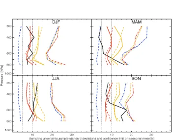
The results are presented in Fig. 8, similar to Fig. 5 for Frankfurt. Over Windhoek, the vertical profiles of the sam-pling uncertainty and the sample standard deviation do not present the well-marked C-shape profiles seen in Figs. 5 and 7. At the highest levels, the ozone variability observed
Table 4. Number of profiles collected per season over the 14 yr period 1995–2008 by the MOZAIC aircraft over Frankfurt, Vienna, Paris, New York, Boston, Tokyo and Osaka. Numbers in parenthesis are the average numbers of profiles collected per season per year.
City (Period) DJF MAM JJA SON Total Frankfurt (1995–2008) 3013 (215) 3026 (216) 3406 (243) 3231 (231) 12 676 Vienna (1995–2006) 867 (62) 1136 (81) 1517 (108) 1245(89) 4765 Paris (1995–2004) 1040 (74) 961 (69) 1062 (76) 1090 (78) 4153 New York (1995–2006) 762 (54) 778 (56) 846 (60) 863 (62) 3249 Boston (1995–2006) 198 (14) 190 (14) 332 (24) 298 (21) 1018 Tokyo (1995–2006) 307 (22) 410 (29) 455 (33) 346 (25) 1518 Osaka (1995–2006) 293 (21) 349 (25) 400 (29) 409 (29) 1451
Fig. 8. Same analysis as in Fig. 5 (Frankfurt) but for Windhoek.
from the Windhoek profiles is much lower than those from the Northern Hemisphere sites. This could be the result of a lesser influence of stratospheric mixing at these altitudes, as the tropopause is much higher in the tropics (around 100 hPa). At the lowest levels, the ozone levels and variabil-ity are also lower than those seen over the Northern Hemi-sphere cities.
Regarding the sample standard deviation (dot-dashed lines), the profiles are similar whatever the frequency. The seasons DJF and MAM show different shapes than in JJA and SON. These differences could be linked to the migration of the inter tropical convergence zone (ITCZ), leading to me-teorological and chemical differences between the wet and dry seasons respectively. In the 600–300 hPa layer, the sam-ple standard deviation is enhanced (up to 30 %) during the winter and fall. During these periods of the year, the ITCZ, located in the Southern Hemisphere, is associated with deep convection, resulting in significant emissions of NOx from
lightning (e.g. Bond et al., 2002). These irregular convective systems contribute to the modulation of ozone production in the upper troposphere (e.g. Edwards et al., 2003; Sauvage et al., 2007) and hence lead to higher ozone variability com-pared to dry months (such as JJA) over Windhoek (J.-P. Cam-mas, personal communication, 2011). From the surface to
300 hPa, the sampling uncertainty calculated for Windhoek is around 8 % and 12 % for the 12 and 4 profile-a-month fre-quencies respectively. These values are similar to what was found in the free troposphere (between 800 and 500 hPa) at the Northern Hemisphere midlatitudes.
For this tropical site, the sampling uncertainty and the 95 % confidence interval of the subsample seasonal mean are close (a difference of less than 5 percentage points). Here, the IAV is of the same magnitude or lower than the sam-pling uncertainty for both frequencies, except in the lowest levels in SON. Fall is the burning season in this region (e.g. Sauvage et al., 2007), and Windhoek is under the influence of important sources of ozone precursors from biomass burning, the magnitude of which may vary from one year to another. However, further study would be needed to better understand the processes controlling the ozone vertical distribution in this area, which is beyond the scope of this study.
7 Conclusions
We have used high frequency MOZAIC data sets to discuss the effect of sampling in the analysis of ozone vertical pro-files in order to estimate the uncertainty that arises when us-ing low time resolution data sets such as ozone sondes. We subsampled the MOZAIC profiles at two typical ozone sonde frequencies, 4 and 12 profiles a month. We performed a de-tailed analysis using the Frankfurt data set, as this is the best documented airport. In addition, we used other northern mid-latitude sites to generalise our findings, and the Windhoek, Namibia data set to discuss a tropical case.
We defined the climatological sampling uncertainty as 2.5 · ssamp,Nf
seas,clim, where s samp,Nf
seas,climis the standard deviation of the
distribution of the differences between the subsample sea-sonal means and the overall mean. This metric has been de-rived per season and per pressure levels. As expected, the sampling uncertainty is higher at the lower time resolution.
The vertical profiles of the average sample standard de-viation have a well-marked C-shape for all the Northern Hemisphere sites, which suggests higher variability of ozone in the lowest and highest levels, probably due to local an-thropogenic pollution events and the potential impact of
stratosphere-troposphere exchange, respectively. As a result, the sampling uncertainty presents a similar shape. The lowest uncertainty is found in the free troposphere at 700 hPa, with values around 5 and 10 % for the 12 and 4 profile-a-month frequencies respectively over Frankfurt. As a consequence, this level is the best candidate for observation comparison and model evaluation purposes in the northern mid-latitudes. For the tropical case (Windhoek), the sampling uncertainty in the free troposphere is around 8 and 12 % at 12 and 4 profiles a month respectively.
We found that: (1) at a 12 profile-a-month frequency, the sampling uncertainty drops below the measurement accuracy (5–10 %) in the free troposphere, while at 4 profile-a-month the sampling uncertainty is generally higher than the mea-surement accuracy and should be considered, (2) the ple standard deviation remains the same whatever the sam-pling frequency, (3) the climatological samsam-pling uncertainty is similar to the average 95 % confidence limit on the sub-sample seasonal mean detected by a subsub-sample, and (4) the 95 % confidence interval of the seasonal mean produced by a sample (as derived in this study) will most probably contain the true mean value and should be used for observation to model or observation comparisons.
We discussed the accuracy of low time resolution measure-ments to detect ozone variations at different time scales. Over Frankfurt, we concluded that: (1) the seasonal cycle is well observed even at the lowest frequency, (2) the IAV signal is generally too low, and consequently masked by the sampling effect, (3) the trend derived over the 11 yr period 1998–2008 varies significantly in magnitude and even in sign with the samples. As a consequence, apparent discrepancies between sites might be attributed to a low frequency sampling in some cases (even though geophysical variations or differences in measurement strategy may also interfere).
These results are valid for the European region, which is under the influence of similar air masses as those of Frank-furt. They might also apply to other northern midlatitude sites such as in North America.
Our results suggest that the sampling frequency should be taken into account for further discussion of observed varia-tions and for observation comparisons or model evaluation. This also strengthens the need to have model outputs on the dates of the sondes for model evaluation, as monthly mean comparisons may be biased by the sampling.
To conclude, this study highlights the significant effect of sampling when using low time resolution measurements. We provide estimates of the sampling uncertainty that arises from such data sets, and we believe that these estimates should be considered for observation comparison and model evaluation. This study strengthens the need for regular and high frequency measurements of tropospheric ozone (at least every two or three days). These high frequency ozone obser-vations are the key to obtaining accurate obserobser-vations of the inter annual variability and decadal changes in ozone
centrations and to better understand changes in ozone con-centrations.
Acknowledgements. The National Center for Atmospheric
Re-search is operated by the University Corporation for Atmospheric Research under the sponsorship of the National Science Founda-tion. The authors acknowledge the strong support of the European Commission, Airbus, and the airlines (Lufthansa, Austrian, Air France) who carry free of charge the MOZAIC equipment and perform the maintenance since 1994. MOZAIC is presently funded by INSU-CNRS (France), M´et´eo-France, and Forschungszentrum (FZJ, J¨ulich, Germany). The MOZAIC data base is supported by ETHER (CNES and INSU-CNRS). The authors are grateful to all the agencies that provide ozone sonde data to the World Ozone and Ultraviolet Radiation Data Centre (WOUDC): German Weather Service – Meteorological Observatory at Hohenpeissenberg and Lindenberg, the National Meteorological Institute of the Nether-lands, MeteoSwiss, the Royal Meteorological Institute of Belgium and the Czech HydroMeteorological Institute. The authors are grateful to the two anonymous referees who helped to improve the manuscript.
Edited by: D. Shindell
References
Bond, D. W., Steiger, S., Zhang, R., Tie, X., and Orville, R.: The im-portance of NOx production by lightning in the tropics, Atmos. Environ., 36(9), 1509–1519, 2002.
Chipperfield, M. P., Fioletov, V. E., Bregman, B., Burrows, J., Con-nor, B. J., Haigh, J. D., Harris, N. R. P., Hauchecorne, A., Hood, L. L., Kawa, S. R., Krzyscin, J. W., Logan, J. A., Muthama, N. J., Polvani, L., Randel, W. J., Sasaki, T., Stahelin, J., Stor-larski, R. S., Thomason, L. W., and Zawodny, J. M.: Global Ozone: Past and Present, Chapter 3 in Scientific 25 assessment of ozone depletion: 2006, Global Ozone Research and Monitor-ing Project-Report No. 50, World Meteorological Organization, Geneva, Switzerland, 2007.
Cooper, O.R., Parrish, D. D., Stohl, A., Trainer, M., N´ed´elec, P., Thouret, V., Cammas, J.-P., Oltmans, S. J., Johnson, B. J., Tara-sick, D., Leblanc, T., McDermid, I. S., Jaffe, D., Gao, R., Stith, J., Ryerson, T., Aikin, K., Campos, T., Weinheimer, A., and Av-ery, M. A.: Increasing springtime ozone mixing ratios in the free troposphere over western North America, Nature, 463, 344–348, doi:10.1038/nature08708, 2010.
Eckhardt, S., Stohl, A., Beirle, S., Spichtinger, N., James, P., Forster, C., Junker, C., Wagner, T., Platt, U., and Jennings, S. G.: The North Atlantic Oscillation controls air pollution transport to the Arctic, Atmos. Chem. Phys., 3, 1769–1778, doi:10.5194/acp-3-1769-2003, 2003.
Edwards, D. P., Lamarque, J. F., Atti´e, J. L., Emmons, L. K., Richter, A., Cammas, J. P., Gille, J. C., Francis, G. L., Deeter, M. N., Warner, J., Ziskin, D. C., Lyjak, L. V., Drummond, J. R., and Burrows, J. P.: Tropospheric Ozone Over the Tropical Atlantic: A Satellite Perspective, J. Geophys. Res., 108, 4237, doi:10.1029/2002JD002927, 2003.
Emmons, L. K., Hauglustaine, D., Muller, J.-F., Caroll, M., Brasseur, G. P., Brunner, D., Staehelin, J., Thouret, V., and