Exploiting variable precision in GMRES
Texte intégral
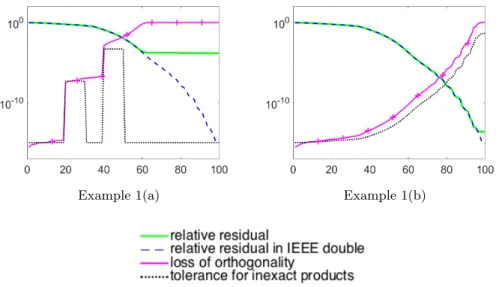
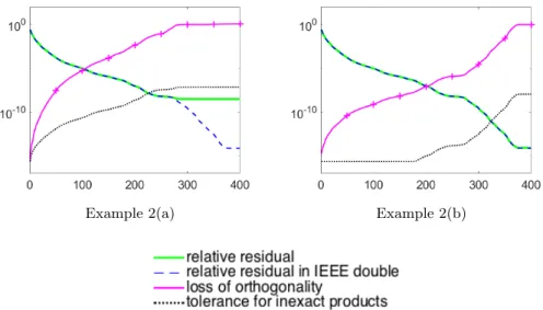
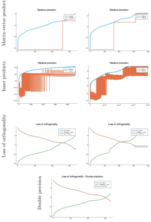
Figure

Documents relatifs
In summary, remember that a wedding always contains the following: two different people (subjects) joined by a ring (que) in an emotion-laden context!. The different categories
According to the aforementioned literature review, proper and thorough research of various vegetation indices in aromatic and herbal plants has to be made, especially for those
Several chemical agents can induce irritation and burn the skin, eyes, and the respiratory tract that may require symptomatic treatment.. Biological toxins may cause
[r]
Poor people cannot afford preventive or curative medical services in countries that do not guarantee health for all; so they not only fall ill (we all do from time to time),
So the Society developed the Pharmacy Self Care programme, designed to provide pharmacists with the training and resources needed to carry out their primary health care
L’archive ouverte pluridisciplinaire HAL, est destinée au dépôt et à la diffusion de documents scientifiques de niveau recherche, publiés ou non, émanant des
The image frames from the video are analyzed using various image processing algorithms to determine particle (fertilizer grain or spray droplet) characteristics.. The
