Mass transfer in Taylor flow: Transfer rate modelling from measurements at the slug and film scale

HAL Id: hal-01924877

https://hal.archives-ouvertes.fr/hal-01924877

Submitted on 16 Nov 2018

HAL is a multi-disciplinary open access

archive for the deposit and dissemination of

sci-entific research documents, whether they are

pub-lished or not. The documents may come from

teaching and research institutions in France or

abroad, or from public or private research centers.

L’archive ouverte pluridisciplinaire HAL, est

destinée au dépôt et à la diffusion de documents

scientifiques de niveau recherche, publiés ou non,

émanant des établissements d’enseignement et de

recherche français ou étrangers, des laboratoires

publics ou privés.

Mass transfer in Taylor flow: Transfer rate modelling

from measurements at the slug and film scale

Colin Butler, Benjamin Lalanne, Krischan Sandmann, Emmanuel Cid,

Anne-Marie Billet

To cite this version:

Colin Butler, Benjamin Lalanne, Krischan Sandmann, Emmanuel Cid, Anne-Marie Billet. Mass

trans-fer in Taylor flow: Transtrans-fer rate modelling from measurements at the slug and film scale. International

Journal of Multiphase Flow, Elsevier, 2018, 105, pp.185-201. �10.1016/j.ijmultiphaseflow.2018.04.005�.

�hal-01924877�

OATAO is an open access repository that collects the work of Toulouse

researchers and makes it freely available over the web where possible

Any correspondence concerning this service should be sent

to the repository administrator:

tech-oatao@listes-diff.inp-toulouse.fr

This is an author’s version published in:

http://oatao.univ-toulouse.fr/19975

To cite this version:

Butler, Colin

and Lalanne, Benjamin

and Sandmann,

Krischan

and Cid, Emmanuel

and Billet, Anne-Marie

Mass

transfer in Taylor flow: Transfer rate modelling from measurements

at the slug and film scale

. (2018)

International Journal of

Multiphase Flow, 105. 185-201. ISSN 0301-9322

Mass

transfer

in

Taylor

flow:

Transfer

rate

modelling

from

measurements

at

the

slug

and

film

scale

C. Butler

a,b

_,

_B.

_Lalanne

a,b

_,

_K.

_Sandmann

a,b,c

_,

_E.

_Cid

a,b

_,

_A.-M.

_Billet

a,b,_∗

a Laboratoire de Génie Chimique, Université de Toulouse, CNRS, Toulouse, France b FERMAT, Université de Toulouse, CNRS, INPT, INSA, UPS, Toulouse, France

c Institute of Multiphase Flows, Hamburg University of Technology, Hamburg, Germany

a

r

t

i

c

l

e

i

n

f

o

Keywords: Mass transfer Taylor flow PLIF-I PIV Lubrication film

a

b

s

t

r

a

c

t

Masstransferinnon-reactivegas–liquidTaylor flowhasbeenstudied atthe unitcell scale withhigh resolutionnon-invasiveexperimentaltechniquesforalargevarietyofhydrodynamicregimesathigh in-ertia(30≤ Reb≤ 1430).Theplanarlaserinducedfluorescencewithinhibition(PLIF-I)techniquehasbeen usedtomeasure thelocaloxygenconcentrationfieldsindifferentliquidphases(tapwater, waterand Breoxsolutionsatdifferentconcentrations)inordertovarytheSchmidtnumberSc.Theconcentration fieldcanbeseparatedintoafilmregion,correspondingtothethinlubricationfilmextendedallalong thechannelwall,andtheremainderoftheliquidwhichmakesuptheslugregion.Ithasbeenfoundthat eventhoughtheglobalmasstransferismainlydrivenbytherateoftransferintheslug,thefilmplaysa significantroleasasourceofoxygen,inadditiontothebubblecaps,tofeedtheslug.

Intheinvestigatedcircularcapillary,fedbymeansofaT-mixer,twocontrastedconfigurationshave beenobservedintheliquidphase(slugsandfilms),dependingonacriticalbubbleReynoldsnumberof ∼ 300,wherethetime-averagedconcentrationfieldsarefoundtodifferconsiderably.ForlargeReynolds number,particleimagevelocimetry(PIV)measurementshaverevealedlowtemporalfluctuationsatthe rearofthebubble,possiblyduetothepresenceofadsorbedcontaminants,thattendstoincreasemixing intheslug.Despitethisdifference,themasstransferdynamicswerefoundtobecontrolledinallcases bytheintensityoftherecirculatingmotionintheslug,whichisdirectlyrelatedtothebubblevelocity forthesecasesofthinfilms.

AnewscalinglawhasbeenproposedfortheoverallSherwoodnumber,basedonReb andSc,which satisfactorilydescribestheoverallmasstransferoftheexperimentalresultsforReb>120toanaccuracy of±11%.

1. Introduction

Manyphysicalsystemsofvariousapplicationsutilisetwo-phase segmentedflows,suchasevaporatingorcondensingdevices.Over the past number of decades, cutting edge technologies of gas– liquid reactorshave appeared, such asmicro-reactors and mono-lithicreactors,whereintermittentseriesofbubblesandslugs (so-calledTaylorflow)arepresent.Thesesystemsofferahigh surface-to-volumeratio,efficientwallheatexchange,inclusionofsatisfying catalytic surface, together withmoderate pressure drop and bet-ter controllability of the reacting system(Machado et al., 2005). When operated inthe Taylorflow regime, thesesystems also al-lowenhancedmasstransferbetweenphases(Kreutzeretal.,2005;

∗ _{Corresponding author at: Laboratoire de Génie Chimique, Université de}

Toulouse, CNRS, Toulouse, France.

E-mail address: annemarie.billet@ensiacet.fr (A.-M. Billet).

Shaoetal.,2010).Althoughthesizeofductsorchannels(eitherof rectangular orcircularcross-section)usedinthesesystems range fromthemicrometretocentimetrescale,theconsidered flowsall showconfinedbubbles(theirshapesdependingonbubblevelocity andfluidproperties)surroundedbyathinlubricationfilm(Taylor, 1961;AussillousandQuéré,2000;FletcherandHaynes,2017).The flow is generallydriven by inertialeffects (Kreutzeretal., 2005), theWebernumberbeinggreaterthanthecapillarynumber.

Formostofthetarget applications,mass transferbetweengas and liquid is a key issue. In particular, it often controls reaction yield inchemical reactors. However, mass transferrate has been shown to strongly depend on capillary diameter and on bubble shape, length and velocity (Haghnegahdar et al., 2016; Hayashi etal.,2014).Inthesameway,twocontributionstogas–liquidmass transferoccursimultaneouslywithinTaylorflow:transferfromthe

Nomenclature

A area(m2₎

C volumetric average concentration in one unit cell (mg/L)

C∗ _{maximumtheoreticalconcentration(mg/L)}

Ca capillarynumber(dimensionless),

µ

lub/

σ

D massdiffusivity(m2_/s)

d capillarydiameter(m)

Eo Eötvösnumber(dimensionless),

(

ρ

l−

ρ

g

)

gd2/

σ

g gravitationalacceleration(m/s2₎

h pixelheight(m)

kL liquidsidemasstransfercoefficient(m/s) KSV Stern–Volmerconstant(L/mg)

N numberofpixels(dimensionless)

n distancenormaltobubbleinterface(m)

mO₂ massofdissolvedoxygen(mg)

L length(m)

[O2] oxygenconcentration(mg/L)

Peb bubblePecletnumber(dimensionless),ubd/D Re_b bubbleReynoldsnumber(dimensionless),

ρ

lubd/

µ

l r radius(m)

r0 radialpositionofrecirculationcentre(m)

r1 radialpositionofdividingstreamline(m)

Sc Schmidtnumber(dimensionless),

µ

l/(

ρ

lD) Sh Sherwoodnumber(dimensionless),kLd/D

t time(s),z/u_b

u velocity(m/s)

ugs superficialvelocityofgasphase(m/s) uls superficialvelocityofliquidphase(m/s) utp two-phasevelocity(m/s),ugs+u_ls Vol volume(m3₎

W relative bubble rise velocity (dimensionless),

¡

u_{b− u}t p

¢

/u_b

We Webernumber(dimensionless),

ρ

lu2bd/

σ

x,y cylindricalcoordinates(morpx)

z distancefromchannelinlet(m)

Acronyms

PIV ParticleImageVelocimetry

PLIF-I PlanarLaserInducedFluorescencewithInhibition

Greek

δ

lubricationfilmthickness(m)

ε

g gashold-up(dimensionless)

µ

dynamicviscosity(Pas)

ρ

density(kg/m3₎

σ

surfacetension(N/m)

τ

shearstress(Pa)

ϕ

rateofmasstransfer(kg/s)

Subscripts

1,2 experimentalmeasurementpositionsalongchannel

b bubble

cir circulationinslug

cor corrected

film lubricationfilm

g gasphase

l liquidphase

s slug

tp two-phase

uc unitcell

bubblecapstoliquidslug,andtransferfrombubbletothe lubrica-tionfilm(Haaseetal.,2016).Eachofthesetwo contributionscan be predominantor negligible,dependingon the situation (physi-cal absorptionof gaswithpossible saturationofthe films, or re-actingwallswithdissolved gasconcentration (Van Baten and Kr-ishna, 2004). Many predictive empirical relations have been de-rived in literature, scaling the Sherwood to the Peclet or Eötvös numbers (Haase etal., 2016; Hosoda et al., 2014; Kastens etal., 2015), orrelatingthe volumetric(liquid side)mass transfer coef-ficientkLa to operational parameters likephase superficial

veloc-ities,bubble andsluglengths (Van Baten andKrishna, 2004; So-bieszuketal.,2012).However,thesescalinglawshavebeenfound to be validin theconditions ofestablishment only. Eachspecific caseorsystemthereforeneedstobeinvestigatedindividually. Fur-thermore,duetothelackoflocaldata,theinsightsintothe com-plexcoupled contributionstomass transfer(Abiev, 2013) arestill rarelyfoundinliterature.Foragoodunderstandingandprediction ofphaseinteractionsandmasstransfer,thelocalphenomenaneed tobe investigatedbyuseofnon-invasive andhighspatial resolu-tiontechniques.

Theplanarlaser-inducedfluorescencetechniquewithinhibition (PLIF-I) has been used for a decade and can be applied to vari-ousgas–liquidsystems,likefreerisingbubbles(Danietal., 2007; Valiorgueetal.,2013;Häberetal.,2015;Jimenezetal.,2013a)or confinedinterfaces(Jimenezetal.,2013b;Roudetetal.,2017; Kas-tens et al., 2017). This technique is based on the use of specific dyeswhosefluorescencecanbe quenchedbythepresenceof dis-solvedgas.

Whenrigorouslyapplied,thistechnique allowsforthe record-ing of images of the dissolved gas concentration field. Instanta-neousandtime-averageddissolvedgas concentrationfields, mea-sured by PLIF-I technique, exhibit well contrasted patterns even close to the gas–bubble interface (Butler et al., 2016). However, the signal to noise ratio may be poor if the laser does not ex-citethedyeatanoptimisedwavelength.Furthermore,incidentand fluorescencelight maybereflected onthe wallandbubble inter-face,leadingtodataprocessingdifficultiesandnon-negligible un-certainties.Toaccountfortheseissues,laserwavelengthshouldbe adjustedtothemaximumdyeabsorption,andaspecificdata pro-cessingmethodologyshouldbeimplementedtotakelight scatter-ingintoaccount.

Additionally,the well-known particle image velocimetry(PIV) technique allows for the possibility to measure the local ve-locity flow fields. This technique is based on tracking the mo-tion of seeded particle groups by pulsed laser illumination and imaging of the light scattering within a small time interval (Charogiannisetal.,2015).Ithasbeenpreviouslyemployedinthe studyofµ-scaleTaylorflow(Kingetal.,2007;Meyeretal.,2014), single Taylor bubbles rising in a column (Bugg and Saad, 2002; Van Hout et al., 2002; Nogueira et al., 2006) and Taylor bubble train flows (Thulasidas etal., 1997;Tsoligkas et al., 2007). These studiesconfirmthepresenceofcounter-rotatingvorticespresentin theliquidphase,whichwasfirstreportedbyTaylor(1961).These vortices drive the mixing process in the slugs (Thulasidas etal., 1997). Most of the studies only describe the time-averaged flow fieldin theslugs;however,an analysisdedicatedtothe instanta-neousflowfieldsbecomesnecessaryatlargeReynoldsnumbersin ordertoquantifyanyfluctuations.

Theaimofthisstudyistoinvestigatethemasstransfer dynam-icsinnon-reactivegas–liquidTaylorbubbletrainflowinacircular capillary,basedontheexperimental concentrationfieldsobtained inhighresolutionbythePLIF-Itechnique,foralargevarietyof hy-drodynamicregimes.Themainadvantageofthismethodisthe ac-quisitionofaccurateinformationaboutmasstransferinbothslugs andfilms,allowing forthe separationoftheirrolestothe overall gasabsorption rate. The studyisrestrictedto regimeswhere the

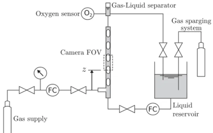
Fig. 1. Schematic of the experimental test-rig.

Taylorflow is stable(i.e. without noticeableoscillation inbubble and/orsluglength)andwhereboththebubbleshapeand concen-trationfieldsareaxisymmetric.Theoccurringphenomenaare fur-therinterpreted thanks to PIV measurements.Based on thisdata ofcontrastingregimesoveralargerangeofparameters,a correla-tionforthe masstransfer rateasa functionof someof the non-dimensionalnumbersrelevantforthisproblemisproposed.

2. Materialsandmethods 2.1. Experimentaltest-rig

Forthedetailedinvestigation ofTaylorbubblesan experimen-talset-uphasbeendesignedthat enableswell-definedand repro-ducibleTaylorbubbleflows.Itconsistsofasinglechannelinwhich thegas–liquidinteractionisobserved(seeFig.1).Thechannelisa verticalglasstubewithacircularcross-section,an internal diam-eterdof3mm (_{± 0.01}mm)anda height of1.2m. Thegasis in-jectedintotheliquidthrough aT-junctionlocatedatthe channel inlet.Itcanbe setupsothateitherascendingordescending con-currentflowcanbegenerated.Thegasflowrateisregulatedbya BrooksSLA580Smassflowmeterconnectedto aWest6100+ dig-ital controller. The liquidphase issupplied froma 20L reservoir tank andis circulatedin aclosed loop by a Tuthill D-seriesgear pump with the flow rate regulated by a Bronkhorst mini CORI-FLOWmassflowcontroller.Thegasbubbles andliquidslugsflow through the channel and are separated at the outlet. The gas is exhausted to the ambient atmosphere and the liquid returns to the reservoir tank. Agas sparging systemis included in the liq-uid reservoir tank which allows the liquid to be completely de-oxygenatedbefore itentersthechannel bycontinuously bubbling nitrogengas.

AUnisenseOX-50micro-sensorprobeconnectedtoaUnisense PA2000amplifierwasplacedatthechanneloutlet.Thissensorwas usedtomeasurethetotalmasstransferalongthechannellength.

Intheseexperiments,oxygenwasusedasthefluidforthegas phase. For reference and calibration purposes, nitrogen gas was alsoused. Forthe liquidphase, tapwaterora water-Breox 75W 55,000solutionwasused.Breox75W55,000isaproductsoldby BASF SE,called“polyalcoxyther” or“Tergitol” (CAS number 9003-11-6). It is a block co-polymer of ethylene glycol and propylene glycol, whichoffers a highviscosity (upto 60Pas at40 °C) and is completely soluble inwater. It was used to vary the viscosity oftheliquidphaseandhencetheSchmidtandCapillarynumbers. 5%and10% m/mBreoxinwatersolutionswereprepared.The liq-uidphysicalpropertiesofthedifferentliquidsolutions(containing thefluorescent dyeusedforthePLIF-Imeasurements)were mea-suredin-houseandarepresentedinTable1.Themassdiffusivities

Table 1

Liquid physical properties at 25 °C.

Liquid ρ µ± 4% σ D

(kg/m 3 ) (Pa s) _{(N/m) (m} 2 /s)

Water 998 1.05 × 10 -3 _{71.2 × 10} -3 _{2.00 × 10} -9

5% m/m Breox-water 1006 4.20 × 10 -3 _{52.2 × 10} -3 _{1.70 × 10} -9

10% m/m Breox-water 1012 9.20 × 10 -3 _{52.0 × 10} -3 _{1.31 × 10} -9

ofwater-Breoxsolutionsweremeasuredfollowingtheprotocol de-scribedinXuetal.(2017).

Rheologyofthetwowater-Breoxsolutions weremeasured un-derdifferentappliedshearstresses

τ

.For0.1Pa_≤

τ

≤ 20Pa, viscos-itycanbeconsideredasconstant,hencethesesolutionsbehaveas Newtonianfluids,whereas,forlower

τ

,shearthinningisobserved. InourexperimentswithBreoxsolutions(seefulllistofregimesin Table2),themaximumvalueof

τ

atthechannelwallliesbetween 0.9Pa(regime11)and6.8Pa(regime14).Thus,thelinearityofthe radialprofileof

τ

inatubeshowsthatthehypothesisofa Newto-nianfluidisvalid,providedx_{≥ d}/18intheworstcondition(regime 11); wewillthereforeassume auniformviscosityfortheseBreox solutionsinthewholecapillaryforregimes11–14.

2.2. Imagingsystemsandsetup

Inordertokeepthecomplexityoftheexperimentalsetupand testingtoaminimum,thePLIF-I,PIVandshadowgraphy measure-ments were not performed simultaneously. The PLIF-I and shad-owgraphyexperimentswereconductedduringthesametest cam-paign for the mass transfer measurements. The experimental set up allows forthecaptureofthePLIF-Iandshadowgraphy images one afterthe other without anymovement ofequipment or dis-turbance of the flow inthe channel. It was simply necessary for therequiredlightsourcetobeactivatedandthecamerasettothe corresponding frequencyofacquisition.ThePIVexperimentswere conductedduringasecondtestcampaignforthevelocity measure-ments.

A glycerolfilled visualisationboxwas placedaround theglass tube duringtheexperiments. Asthe refractive indicesofglycerol andglassarealmost identical,anyrefractionorreflectionoflight asit passesthrough thechannel wallsbecomesnegligible (Häber etal.,2015;Thulasidasetal.,1997).

2.2.1. Shadowgraphysetup

The shadowgraphy technique is a well-known visualisation technique which involves illuminating the subject of study by a diffuse light source and recording images of its shadow (Settles, 2001). The camera used for the shadowgraphy imaging was aPCO Edge5.5sCMOScamera.Itsresolutionwas reducedto 2560_{× 402} pixelstoimage thechannel areaofinterest onlyand allowforahigherfrequencyofacquistionof100Hz.Anexposure time of 100 µs was usedto effectivelyfreezethe flow. The cam-era wasfittedwitha Nikon105mm macrof/2.8lensandaseries ofextension tubeswithatotallength of68mm.A120_{× 160}mm PhloxLEDpanelwasusedasacontinuouslightsource.Itwas po-sitioneddirectly behindthechannel, perpendicular totheaxis of thecamera.

2.2.2. PLIF-Isetup

The basic principle ofthe PLIF-I technique takes advantage of the fluorescent quenchingbehaviour of molecular oxygen to cer-tainfluorophores.ThisquenchingisgovernedbytheStern–Volmer equation

I0,x,y

Ix,y =

where I0 andIare thefluorescent intensities in theabsence and

thepresence(respectively)ofthedissolvedoxygen,[O2]isthe

con-centration ofdissolved oxygen, KSV is theStern–Volmer constant,

andxandycorrespondtothespatialcoordinatesofagivenpixel onthe camerasensor.Thefluorescent tracerusedinthese exper-iments isDichlorotris (1,10-phenanthroline)ruthenium(II) hydrate ([Ru(phen)3]) (CAS No. 207802-45-7). This tracer has been used

previously intheliteratureforoxygenationmeasurements (O’Neal etal.,2004;Huntsovaetal.,2014;Jimenezetal.,2014;Jankeand Bauer,2017).Thetracerisdirectlysolubleintheliquidphaseand is used at a low concentration of 50mg/L. As a consequence, it doesnotsignificantlyaltertheliquidproperties,andpresents con-stantcalibrationproperties(Jimenezetal.,2014).

Thelightsourceusedtoexcitethistracerwasan Opotek Opo-lette355tunablelasersystem.Theadvantageofusingthissystem isthatit cangeneratewavelengthsoverabroadrangeand there-foreallowsforthetuningofthelaserlight tothemaximum exci-tation frequency of the tracer beingused. By exciting the tracer at its maximum absorption wavelength of 450nm, the resulting emission is maximisedand imageswithexcellent dynamic range areproduced.Theemissionintensitiesarerelatedtothedissolved O2concentrationbyEq.(1).Bycomparingimagesproducedwitha

Nd:YAGlaser(wavelengthof532nm),itwasfoundthatthose pro-ducedwith theOpolette laser (5 mJ) hada dynamic rangethree times greater. Amotorised attenuator assures the stabilityofthe laser energy pulses, with a measured standard deviation of less than5%betweenpulses.

The laser system was equipped with a lens system which produces a diverging laser sheet with a measured thickness of 280µm. Thelight sheetwas positionedto passthrough the cen-trelineofthechannelandperpendiculartotheaxisofthecamera. Asmentionedatthestartofthissection,theshadowgraphyand PLIF-Iimagingwasconductedduringthesamecampaign,therefore thesamecamerasetupwasused.Thecamerawassettoan acqui-sition frequency of 20Hz with an exposure time of 100 µs. The frequencyofacquisitionislimitedbythemaximumrepetitionrate of thelaser system. The excited lifetimeofthe Ruthenium tracer complex is <20 µs (Nakamaru, 1982) meaning there can be no cumulative effectofthefluorescentsignal duetomultiple excita-tionsfromthelaser.A540nmOD6highpassfilterwasplacedin front ofthecameratoblock thelightatthelaserwavelengthbut allowtheresultinglightatthefluorescentwavelengthstopass.

2.2.3. PIVsetup

Time-resolved particle image velocimetrymeasurements were carriedoutinthesameplaneasthePLIF-Iimages,passingthrough thecentrelineofthechannel.APegasuslaserfromNewWave de-livering 2_{× 8} mJ at 532nm, operating at 500 Hz, and a CMOS camera RS3000 (Photron) with a resolution of 1024× 220 pix-els were used.The camera was equippedwiththe same105mm Nikon lens, extension tubes and high pass filter that were used forthePLIF-Imeasurements.Fluorescentpolystyreneparticles (PS Fluo-Red) witha meandiameterof 10µm were used asseeding particlesintheliquidphase.Thesystemallowedtheacquisitionof pairsofimagesatarateof500Hz.Thesepairswereanalysed us-ing Davis 8.4software(Lavision) using75% overlapping windows of32_{× 32}pixels,yieldingfieldsof128_{× 21}vectorswithaspatial resolutionof0.135mm(0.045d)intheaxialdirection.

2.3. Experimentalprocedureformasstransfermeasurements

The mass transfermeasurements are obtained fromthe shad-owgraphyandPLIF-Iimaging,aswellasfromtheO2 micro-sensor

probe. Pure O2 was used asthe gas phase. Givengas and liquid

flow rates were set on the corresponding controllers, and 5000 shadowgraphyandPLIF-Iimageswererecordedoncetheflowwas

Fig. 2. An example of a calibration curve for determination of the Stern–Volmer constant for a pixel from the interrogation window; also shown the calibration curve of the O 2 sensor probe (water as liquid phase).

stabilised.Examplesofrecordedinstantaneous shadowgraphyand PLIF-Iimagesare showninFigs. 3and4.This procedurewas re-peatedforalloftheTaylorflowregimesobservedinthisstudy.The positionz ofthecamera andthelaserwas then moved toa sec-ondpositionacertaindistancefurtherawayfromthechannelinlet andthemeasurements wererepeated forthesamerangeof flow rates.ThismeansthatfourO2 concentrationvaluescanbe

quanti-fiedalongthechannellengthforagivenflowregime:attheinlet (z₌0),attwopositions(z1,z2)alongthechannel(valuesofz1and

z2dependontheconsideredregime),andattheoutlet(z=1.2m).

A number of important calibration steps are required for the masstransfermeasurements. Thefirstincludesthe determination ofKSV in Eq. (1)at each of the two positions along thechannel

forthe PLIF-I images.The calibrationprocedure involves saturat-ingtheliquidatknownO2 concentrationvaluesandrecordingthe

resultingfluorescenceby thecamera(Danietal., 2007).Thiswas achievedby bubblingmixturesofO2 andN2 gasinsidetheliquid

reservoir at0% (pure N2), 5%, 10%, 21%(air)and 100%(pure O2)

forlongdurations(morethan30min)toensuresaturationofthe liquidphase.Saturation(andthussteadystate)was confirmedby thestabilisationoftheO2 sensorsignal.Foragivenconcentration,

100 imageswere used to createan average image and thevalue ofKSV could then be determined by alinear regressionfit ofthe

data,pixelbypixel,asshowninFig.2,wheretheslopeoftheline isequaltoKSVforagivenpixel.Thistypeofcalibrationprocedure

thereforeaccountsforlaserlightsheetnon-uniformity,absorption, pixelresponse non-uniformityandlens vignette(Valiorgueetal., 2013;Websteretal.,2001).Atthesametimeasthesecalibrations, theO2 sensorprobewasalsocalibrated.Theelectricalsignalfrom

theprobewasrelatedtotheknownO2 concentrationsusinga

lin-earregressionfit,asshowninFig.2.

Aspatial calibrationstepwasnecessarytodeterminethe mag-nification factor to convertfrompixels to physical units of mea-sure. To do this, a checkerboard pattern, consisting of a grid of 15_{× 15}squares,each193µm(_±0.68µm)inwidth,wassuspended insidethechannelinthecamera’sfieldofview.Duetorefraction effectsbetweentheglasschannel andinternalliquid,pixelwidth in the radial direction increases with distance from the channel axialcentreline. Theseeffects havebeentakenintoaccount using the Snell–Descarteslaw, which involves a seriesof trigonometric operationscoupledwiththegeometrical opticsoflight refraction (MacGiollaEainetal.,2013). Aconstant magnificationfactorwas appliedintheaxialdirection.

Fig. 3. Shadowgraphy image processing using data for regime 9.

Fig. 4. PLIF-I image processing using data for regime 9.

In order to account for light scattering effects due to the re-flection and refractionof thelaser light asit passesthrough the bubble interface, the mass transfer measurements were repeated by replacing O2 with N2 asthe gas phase. This scatteringeffect

can be seen in Fig.4(a) as theareas of increasedintensityclose tothebubbleinterface. Itisassumedthat nomasstransfertakes place between the N2 gas bubbles andthe de-oxygenatedliquid

phase,andtherefore,thereshouldbe nospatial variationsdueto quenchingofthe fluorescence signalas thedissolved O2

concen-trationisuniformandequalto0.Asaconsequence,theN2images

canserve asareference, wherebythelevelof increasedintensity canbequantifiedandthenremovedfromtheO2 images.The

pro-ceduretoapplythiscorrectionisdetailedinSection3.1.2and val-idatedinSection3.1.3.

3. Imageprocessing

3.1.Masstransfermeasurements

In order toextract the data relatedto the masstransfer phe-nomena occurringbetween the two fluids, significant processing oftheshadowgraphy andPLIF-Iimageswas required.All the im-ageprocessingwasperformedusingMATLAB,andcomputationally intensivetaskswereperformedusingaGPUbyintegratingcustom CUDAkernels.

3.1.1. Shadowgraphyimages

The shadowgraphy images were used to determine the phys-ical characteristics andsome hydrodynamic dataof a given flow regime.

The firststep inthe processingofall theimagesis the deter-mination ofthe phases. The locations of the solid channel walls (seenasthedarkverticalbandsontheleftandrightoftheimages inFig.3(a)) werefound fromanedge detectionalgorithm,where an edgelocationwas associatedwithalocalpeakinthegradient imageintensityvaluesintheradialdirection.

Tofindtheposition(s)ofthebubble(s)ineachimage,each im-agewascross-correlatedwithtemplateimagesofthebubblenose andtail(seeFig.3(b)).Analgorithmwasthenusedtosortthe cal-culatedbubblenoseandtailaxialpositionsineach imageandto understandtheorderofthephases,i.e.fromthebottomtothetop ofan image:partial gasbubble– liquid slug– gasbubble – par-tialliquidslug, orpartialliquidslug– gasbubble– partialliquid slug, etc. This informationwas importantasit was then used to calculatethebubbleandsluglengths,LbandLs,respectively,with

theaidofthespatialcalibration.TheaveragelengthLucoftheunit

cell can then be deduced foreach studied regime, as definedby

Luc=Lb+Ls.

To isolate the complete gas–liquid bubble interface, a back-ground image was firstly subtracted from the instantaneous im-age.Thebackgroundimageconsistsofanimagewithnogasphase present (see Fig 3(c)). The result of the subtraction was an im-agewhichonly containsthe gasbubble(s)(seeFig.3(d)). Usinga technique similartothatforthechannel wallpositions,the inter-facecouldthenbetraced.Assumingaxialsymmetry,anintegration ofthe interface profileaboutthecentreline givesthe bubble vol-ume.Thusthevalueofgasholdup,

ε

g=Vol_b/Voluc,wascalculated, whereVoluc=

π

d2_L

uc/4.

The time-averagedbubblevelocity ub was calculatedfromthe

displacement of a bubble from one image to the next and the camera frequencyofacquisition. Thedisplacement isobtainedby cross-correlating twosuccessive image frames. Thismethodgives aprecisionof1_{× 10}-3_{m/sinthecalculationofu}

b.

3.1.2. PLIF-Iimages

ThePLIF-Iimageswereusedtodeterminetheconcentrationof dissolvedoxygen[O2]intheliquidphase.Theimageprocessingis

summarisedinFig.4.

As mentioned earlierin Section 2.3, two setsof PLIF-I images were requiredfor a given Taylor flow regime – one using O2 as

the gas phase, and a second using N2. The N2 images served as

referencesinordertoquantifythescatteredlightsoitcouldthen becorrectedforintheO2 images.

The pattern and intensities of scattered light were found by subtracting the N2 images with a background image. The

back-groundimage is definedasan image withno gasphase present, andinwhichtheliquidiscompletelysaturatedwithN2.Foreach

pixel oftheimage,thiscorresponds to I0,x,yinEq.(1).The

scat-tering patternimage (see Fig.4(c)) showsthezonesof increased intensityclosetothebubbleinterfaceastheareasofincreased in-tensityintheliquidphase.Thescatteringpatternimage was nor-malised by dividingit bythe instantaneousN2 image tofindthe

relativeincrease inintensity,pixel-by-pixel.Atime-averaged scat-teringpatternimage (see Fig.4(d)) was thencreated by translat-ing theimagesintheaxialdirectionsothebubblesandslugsare aligned. This translationdistance was determined foreach image by cross-correlating an image with templates ofthe bubble nose and tail, similar to the process used for the shadowgraphy im-ages. Ofthe 5000images recorded,only those which hada slug length exactly equalto the mediansluglength, determined from the cross-correlation step,were usedto createthe time-averaged images.Thiswasdonetoensuretheslugsandquenchingpatterns alignedcorrectlywhentheyweretranslatedbeforetime-averaging. On average,approximately400 ofthe 5000 imageswere used in thefinaltime-averagedimages.

Then,inordertocorrecttheinstantaneous O2 images,the

fol-lowingequationwasappliedpixel-by-pixel,assumingthat,ateach considered pixel,thescatteringeffectshave thesamerelative or-derofmagnitudeforanyaveragevalueof[O2],

Icor,x,y=Ix,y

·

1₋

µ

_¯I

N2,x,y− ¯I0,x,y

¯IN2,x,y

¶¸

(2) whereIcor isthe corrected pixelintensity, Ix,y is theuncorrected

instantaneous intensity, and the terms in the round parenthesis correspond to the normalised scatteringpattern image produced from the subtraction process of the N2 images and the

back-ground image. After applying Eq. (2), the discontinuitiespresent inquenchingpatternsarenolongervisible(seeFig.4(g)).

Beforecreatingthetime-averaged[O2]image,theinstantaneous

imageswerefirstconvertedfromgrayscaleintensityvaluesto[O2].

Forthis, Eq.(1)isusedastheKSVcalibrationisdesignedtowork

pixel-by-pixel.Fig.4(h) showsthe imagesconverted into[O2]/C∗.

This maximum value C∗ _{is the theoretical saturation of [O2] in}

watercalculated fromHenry’ s law (Sander, 2015), andused for calibration.In the casewhereliquid phase isa mixture ofwater andBreox (regimes11–14),C∗ _{is unknown.It can be assumedto}

be close to the C∗ value for water, as the mixtures contain 10% of Breox at maximum. However, it is preferred here to express all concentration data through the calibrated normalised values [O2]/C∗inthesecases.Thetime-averagedimagewas createdfrom

translatingtheinstantaneousimagesalongtheaxialcentreline. Theareaofinterestinthetime-averaged[O2]imageistheunit

cell, i.e. one complete bubble and slug. The data hidden by the bubbleshadowduringthePLIF-I measurements,seen asthearea ofreducedintensityto therightof thebubbles inFig.4,aswell asthebubbleitself,cannotbeexploited.However,astheunit cell isexpectedtobe axisymmetric,thetotalmass ofdissolvedO2 in

theliquidphase canbe calculatedby thesummation ofthe con-centrationofeachpixelmultipliedbythecylindricalshellvolume ofeachpixel, mO2= Ny X y=1 Nx X x=1 [O2]x,y

£π¡

r2x,y− rx2−1,y

¢

h

¤

(3) where r is the radius of a cylindrical shell, h is the height of a pixeland N isthe numberofpixels. As statedabove, dueto the axisymmetry,thepixelswereintegratedonlyonthelefthandside ofeachimagewithrespecttotheaxisofsymmetry.Notethatfrom knowingthepositionsofthebubblenoseandtailfromthe cross-correlationstep,andtheshapeofthebubbleinterface,determined fromtheshadowgraphyimagesinSection3.1.1,thevaluesof[O2]

insidethebubblewerefirst setto0beforeapplyingEq.(3)soas nottobeincludedinthecalculationofmO₂.

3.1.3. Scatteredlightimagecorrectionvalidationtests

Inordertoassessthecorrectionmethodologyusedduringthe PLIF-Iimageprocessing,describedintheprevioussection,aTaylor flowregimewas generatedwithknowngasandliquid concentra-tions. Thiswas achievedby pre-saturating waterin the reservoir withairandusingairasthegasphase.Whenthetwophases en-terthechannel,astheyareequilibratedvaluesof[O2],noO2mass

transfertakesplace,howeverthelightscatteringphenomenonwas stillpresentandresultsinanincreasedintensitysignalasseenby thecamera.

Thetime-averagedmassofdissolvedO2wascalculatedforthis

regime, both with andwithout the application ofEq. (2).It was then compared to the theoretical value of the mO2 in the iden-ticalliquidslug completelysaturated withair.For thiscasewith nocorrection,thetotal valueofmO₂ was underestimatedby 22%,

Table 2

Summary of experimentally measured Taylor flow regimes.

Regime No Liquid phase Config. ugs uls utp ub Reb Sc Ca We (m/s) (m/s) (m/s) (m/s) 1 Water Asc. 0.022 0.020 0.041 0.042 1.2 × 10 2 _{5.3 × 10} 2 _{6.1 ×10} −4 _0.1 2 Water Asc. 0.047 0.039 0.086 0.092 2.6 × 10 2 _{5.3 × 10} 2 _{1.4 ×10} −3 _0.4 3 Water Asc. 0.045 0.079 0.124 0.140 4.0 × 10 2 _{5.3 × 10} 2 _{2.1 ×10} −3 _0.8 4 Water Asc. 0.088 0.098 0.186 0.210 5.9 × 10 2 _{5.3 × 10} 2 _{3.1 ×10} −3 _1.9 5 Water Asc. 0.084 0.149 0.233 0.274 7.8 × 10 2 _{5.3 × 10} 2 _{4.0 ×10} −3 _3.2 6 Water Asc. 0.177 0.118 0.295 0.338 9.6 × 10 2 _{5.3 × 10} 2 _{4.9 ×10} −3 _4.8 7 Water Asc. 0.222 0.118 0.340 0.393 1.1 × 10 3 _{5.3 × 10} 2 _{5.8 ×10} −3 _6.5 8 Water Asc. 0.274 0.141 0.415 0.501 1.4 × 10 3 _{5.3 × 10} 2 _{7.4 ×10} −3 _10.6 9 Water Asc. 0.103 0.143 0.246 0.283 8.1 × 10 2 _{5.3 × 10} 2 _{4.2 ×10} −3 _3.4 10 Water Des. 0.056 0.161 0.217 0.240 6.8 × 10 2 _{5.3 × 10} 2 _{3.5 ×10} −3 _2.4 11 5% m/m Breox-water Asc. 0.042 0.039 0.081 0.097 7.0 × 10 1 _{2.5 × 10} 3 _{7.8 ×10} −3 _0.5 12 5% m/m Breox-water Asc. 0.157 0.118 0.285 0.373 2.7 × 10 2 _{2.5 × 10} 3 _{3.0 ×10} −3 _8.0 13 10% m/m Breox-water Asc. 0.039 0.078 0.078 0.097 3.2 × 10 1 _{6.9 × 10} 3 _{1.7 ×10} −2 _0.5 14 10% m/m Breox-water Asc. 0.158 0.118 0.276 0.381 1.3 × 10 2 _{6.9 × 10} 3 _{6.7 ×10} −2 _8.5

Fig. 5. Relative bubble rise velocity experimental measurements compared to cor- relations from literature.

of5%whencomparedtothetheoretical value.Theformer under-estimationisduetotheincreasedsignalintensityandthe reduc-tioninobservedfluorescencequenching.Thelattercanbeadopted astheexperimental[O2]uncertaintyvaluesforthePLIF-I

measure-mentsinthiswork.

3.2. PIVimages

As mentioned inSection 2.2.3,double-frame PIV images were acquiredataframerateof500Hz.Thetimedelaybetweeneach frame was chosen depending onthe maximumparticle displace-ment for each flow regime, andranged from 140 to 1600 µs. In ordertoprovideaverage quantities,eachofthedouble-frame PIV imageswas,first,translatedtothesamereferencepositioninthe fieldofview.Thiswasachievedbytemplatematchingofnose bub-bleinPIVimages,asforthePLIF-Iimages.Ina secondstep,each velocityfieldwas calculatedandthentime-averaged. Mean veloc-ityandroot-mean-squarevelocityfieldscanbecalculatedforeach flowregime fromathousanddoubleframePIV images.Statistical convergencehasbeencheckedformeanandfluctuatingvelocities. Asformasstransfermeasurements,thesamespatialcalibration procedurewasappliedtoPIVvelocityfields.

4. Resultsanddiscussions

In thiswork, 14differenthydrodynamic regimeswere consid-ered,eitherascending ordescending con-current flows,asshown below in Table 2. The geometry of Taylor flows obtained were formed of bubble trains composed of unit cells of length 2.9_≤

Luc

d ≤ 5.7,includingbothshortandlongslugs,whoselengthswere

in the range 0.7_≤Ls

d ≤ 3.1. The hydrodynamics are characterised

byarangeofmoderatetohighReynoldsnumbers(basedon chan-nel diameter andbubblevelocity) 30_{≤ Reb≤ 1430}anda range of low capillary numbers6_{× 10}−4_{≤ Ca≤ 6× 10}−2. Thesevaluesare associated toWeber numbers0.1_{≤ We≤ 10.6.}Thus,inertial forces are always dominantcomparedto theviscous forcesinthese ex-periments.Insomecaseshowever,capillarityisdominantover in-ertia (low We) such asforregimes1–2–3–11–13,whereas inertia dominates capillarity for all other regimes (large We). Note also that the Eötvösnumberisalways of order1(1.2_{≤ Eo≤ 1.7).} Con-cerningmasstransfer,throughtheuseofdifferentliquids(tap wa-ter,solutions ofBreox5% andBreox10%),theSchmidt numberis variedovertherange520_{≤ Sc≤ 6940.}

4.1. Relativebubblerisevelocity

The bubblerise velocity isan importantparameterin the un-derstandingofTaylorflowasitimpactsmasstransferintothe liq-uid phase. Fig. 5 compares the relative bubble rise velocity, de-finedbyW₌

¡

u_{b− u}t p

¢

/ub,whereutpisthetwo-phasesuperficial

velocity andubthebubblevelocity, withsomeofthe

experimen-talcorrelationsavailableinliterature.Amongavailableresults,the first lawW_{∼ Ca}12, proposed by Fairbrotherand Stubbs(1935) is included, which has been shown to be validup toCa₌0.09 by Taylor (1961). Bretherton (1961) has proposed a differentscaling lawW_{∼ Ca}23. Morerecent correlationsare also plottedinFig. 5, includingthoseofLiuetal.(2005),validfor2× 10−4_<Ca<0.39,

andofAbiev(2013),validforbothsmallandlarge Ca,butalways low We.Fig.5showsthatfortheregimesinthiswork,where in-ertiaisnotnegligible,thevaluesliebetweenthepredictionof cor-relationsofLiuetal.(2005)andAbiev(2013).Notethatthevalue of regime 1 hasa larger errorbar due to the fact that the flow controllerswereoperatingclosetotheminimumoperatingpoint.

FollowingAbiev(2008),inthecaseofslugflow,thelocalmass conservation equation (continuity equation) can be written for eachphaseseparatelyandintegratedinacrosssectionofthe cap-illary based on the knowledge of the average surface fraction of each phase;then,an axialintegrationoveroneunitcelllength in additiontotheflowincompressibilityconditionimposesthat

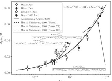
Fig. 6. Experimental liquid film thickness measurements.

whereu_film istheaveragevelocityinthelubricationfilm,andA_film, AbandAarerespectivelytheareaoccupiedbythefilm,thebubble

andthe wholecross section.This exactbalance, Eq.(4),between the different volumetric flow rates can be simplified in the case ofa gas–liquidslugflow. Indeed,Howard andWalsh (2013) have shownthatthemostimportantparameterplayingontheratioof magnitude between the film andbubble velocities is the viscos-ity ratio; in the caseof gas–liquid flows (very high viscosity ra-tio),ufilmcanbeconsideredasnegligiblecomparedtoub

(assump-tion ofstagnant lubricationfilm). Moreover,assuming thatCa≪ 1 asconsideredinthisstudy,i.e.

δ

film≪ d(seeSection4.2),Eq.(4)is

simplifiedto ub utp ≈ A Ab ≈ 1+ 4

δ

film d (5)

Eq.(5)showsagainthatthebubblevelocity isalwayslargerthan the average two-phase flow velocity utp (or slug velocity), and

presents theadvantage toemphasise that the relativebubble ve-locityWandthefilmthicknessarestronglylinkedinthisproblem; thisiswhyauthorslikeHoward andWalsh (2013)haveproposed an iterativeprocess basedonthe existingcorrelationsforthe es-timationofthesetwoflowparameterssimultaneously.Inthenext section,experimentalresultsofthefilmthicknessarecomparedto existingcorrelationsfromtheliterature.

4.2. Liquidfilmthickness

Severalanalyses exist to characterise the thickness of

δ

film of

thelubricationfilmbetweenthebubbleandwall.

Without inertial effects, (We_{≪ 1),} in a regime of Ca_{≪ 1,} the study of Bretherton (1961), based on the lubrication approxima-tion,showsthat

δ

film isgivenbythebalanceofviscous forceand

thepressuregradientthatoriginatesfromthedifferenceof curva-turesbetweenthesphericalbubblecapandtheflatregionparallel tothewall,whichgivesthewellknownlawδf ilm

d/2 ∼ Ca

2

3.Thisstudy hasbeenextendedbyAussillousandQuéré (2000)forhigher val-uesofCa,butalways invisco-capillary regimesunderthe condi-tionCa<1,by using a geometric correctionon the curvature ex-pressionthatyields δf ilm

d/2 ∼

Ca23

1+Ca23

where

δ

film onlydependsonCa.

In the presence of inertial effects (We>1), Aussillous and Quéré (2000)havereportedthat thefilmthicknessincreasedand they have proposed, in this latter case, a correlation based on both Ca and We.Numerical results of Kreutzeret al.(2005) and Heil(2001)haveconfirmedthetrendandhavealsotakeninto ac-count changes in bubble nosecurvature through numerical sim-ulations up to Reb=200. Based on these observations and on

by use of a laser focus displacement meter, a new correlation basedonageometriccorrectionwas proposedbyHan and Shika-zono (2009) which takes into account such inertial effects and relates

δ

film as a function of (Ca, We, Reb), even though only 2

of these parameters are independent. The latter correlation has been confirmed by recent measurements of both Howard and Walsh (2013) – based onhighspeed optical microscopy with re-fractiveindexmatchingwhichshowsanagreementwithlessthan 10%discrepancy,andKurimotoetal.(2017)– basedonhighspeed camera measurements, showing an agreement between_±20% up toRe_b=100.

The measurements in this work, reported in Fig. 6(a), corre-spond to the inertial regime andallow for the extension of the comparison withthe existing predictive correlations up to Re_b=

1430.Itshould benotedthat duetothepointedshaped ofsome of thebubbles, especially athigher valuesof Reb, theliquid film

thicknessisnotalways uniformintheflatbubbleregion andhas been defined asthe minimum distance between the bubbleand thechannelwallobservedintheshadowgraphy images,asshown in Fig. 6(b). The correlation proposed by Aussillous and Quéré (2000)compareswell withourmeasurementsforregimesWe<1, withan averagedifference of15.8%. In contrast,for regimes5–9 which correspond to the highest We (ranging from 3.2 to 10.6), the prediction of film thickness by the correlation of Han and Shikazono(2009)that doesconsiderinertialeffectsis clearly im-proved. It can be observed that the experimental measurements areinverygoodagreementwiththecorrelationofHanand Shika-zono(2009)forallthefluidsconsideredhere,withanaverage dif-ferenceof16.0%,despiteamaximumdifferenceof47%forregime 5.

4.3. Time-averagedvelocityfieldsinslugs

Thevalue ofW,therelativebubblevelocity, isdirectlyrelated to theflow streamlines,asshownby Taylor(1961).Forvaluesof

Ca<0.7and W<0.5 as for all regimes in the present work, the flowpatternsconsistofarecirculatingflowintheliquidslug,with stagnation points existing on the bubble nose. This flow organi-sationisvisualisedbycalculatingthetime-averagedvelocityfield using the PIV technique, and by subtracting the bubble velocity from the time-averagedvelocity utp previously calculated, to

ob-tainthemeanvelocityfieldinthebubblereferenceframe.Fig.7(a) shows this mean velocity field for flow regime 2 superimposed withstreamlines.Twomirroredrecirculationflowpatternsare ob-served andcompared welltothe concentrationpatternsobtained byPLIF-Itechnique forthesameflowregime(seeFig.9).

For regime 2, a radial velocity profile, calculated in the fixed referenceframeisalsopresentedinFig.8.Thismeanvelocity pro-file,extractedathalfwayalongthesluglength,iswell fittedbya parabola,whichisconsistent withthe Poiseuilleflowmodel usu-ally found whenthe sluglength is greater than a few diameters (Thulasidas et al., 1997). As a consequencethe flowin theliquid slugcanbeconsideredtobefullydevelopedforthisregime.

4.4. Time-averagedO2concentrationfields

Thetime-averagedO2 concentrationfieldsmeasured usingthe

PLIF-I technique for the 14 different regimes are presented in Fig. 9.For each regime, the contours closeto the inlet, ata dis-tancez1,andthen atthe second field of view,z2, arepresented.

Thehalfunit cellsextractedduringtheimageprocessingare mir-rored aboutthe axial centreline asone half of the liquid slugis partiallyhiddenbythebubbleshadow(seeFig.4(h)and(i)),and aseachunitcellisobservedtobeaxisymmetric.

A wide variety of hydrodynamicregimes have been explored, where the concentration fields can be seen to vary significantly.

Fig. 7. Experimental PIV time-averaged velocity fields for regime 2 (see Table 2 for regime details).

Fig. 8. Radial velocity profile in the fixed reference frame for regime 2 extracted halfway along the slug length.

Some zonescan begenerallydistinguished. Firstly,inliquidslugs, thereisarecirculationpattern,asmentionedpreviously,which en-surestransportofO2 betweenthetwoconsecutivebubblesofthe

train (see forexample regimes1,2, 11,13 inFig. 9). Then,along the tube axial centreline, a region with a higher concentration than therest oftheslugisgenerallyvisible.This isexplainedby theexistence ofa maximuminvelocityatthechannelcentreline, making convective transport of O2 themost efficient,witha

rel-ative velocityequal to 2ut p− ub whenconsidering an established

Poiseuilleflowintheslug.Finally,alongthechannelwall,the res-olution of the experimental measurements allows for the obser-vation of a thin concentration film: this film is associated with thelubricationfilmbetweentheflatregionofthebubbleandthe wall, but alsoextends along thechannel wall inthe unit cell. In

Fig. 9. Time-averaged and normalised O 2 concentration contour plots. These images have been corrected for scattered light and radial distortion. The half unit cells are

mirrored about the axial centreline. The [O 2 ] values inside the bubble have been set to 0 for clarity.

thisway,forthemasstransport analysis,a continuousfilmalong the channel wall is considered,lying between theradial position of the dividingstreamline in theslug andthe wall, asshown in Fig. 10. This dividing streamline, illustrated by Taylor (1961) and Thulasidas et al.(1997),is the streamlineconnecting the stagna-tionpointsonthefrontandrearofthebubblesurface,whichthus separatesthecirculatingvortexintheslugfromtheliquidfilm at-tachedtothewall.Assuminga Poiseuilleflowintheslug, the ra-dial positionr1 ofthedividingstreamline(Thulasidas etal.,1997)

canbepredictedby r1= d 2

r

2₋ ub ut p (6) ThisstagnantfilmisrichinO2all alongthechannelwallbecause

ofbothradial diffusioninthelubricationfilmincontactwiththe bubbleandefficientaxialconvectivetransportinthevicinityofthe

slidinginterface, due tothe relative velocity betweenthe bubble andthelubricationfilm,whichisclosetoub,whenconsidering a

stagnantfilm.

Astheflowtravelsfromz1 toz2,the[O2]increasesinthe

dif-ferentregions.Theliquidcanbeseentoapproachsaturationatz2

forregimes7and8whicharetheregimesathighestReb.Forthe

regimesof10%Breox(13and14)atthehighestCa,theincreasein [O2]intheliquidfilmcanbeclearlyobservedbecauseofthe

rela-tivelylargerfilmthicknesswhencomparedtotheotherregimes. Regimes 1 and 2 for water, and 11–14 with Breox, show concentration fields similar to what is observed in some nu-merical studies for cases of physical absorption, such as in Shaoetal.(2010)andHassanvandandHashemabadi(2012),with thecentreof thevortex beingthepoint inthe slugwhichisfed theslowest withO2 since diffusion hasto transferO2 across the

Fig. 10. Sketch showing the different characteristic dimensions and areas in the unit cell.

Nevertheless,forregimes3–10,aninterestingfeaturewhich ap-pearsisthepresence ofvorticesofuncharacteristicconcentration levelsintheslug,describedasanareaofrelativelyhigh concentra-tioninthecentreoftheslugsurroundedbyazone oflower con-centration,whichisclearlyvisibleforregime3,7and8for exam-ple.ItisworthremindingherethattheseTaylorflowregimesare notassociatedwithoscillationsofthebubblenoseandthat,even though [O2] fieldspresented in Fig. 9 are time-averaged, the

in-stantaneousfieldshavethesamestructureanddonot showlarge fluctuationsintheconcentrationvalues.Apossibleexplanationfor thesefeaturesisthat theyare associatedwithparticularflow dy-namics,differentfromthatshowninFig.7,whichappearsaftera criticalvalue of aboutReb>300. Thiswill be discussed later.

Be-cause ofthe strong impact of hydrodynamics in the slugon the concentration fields, in the following sections, the local transfer mechanisms are first described for cases of classical concentra-tion fields likethose observed at Reb<300, andcases associated

toanomalouspatternsatRe_b>300arediscussedseparately.

4.5. AnalysisoflocalmechanismsformasstransferatReb<300

Herethemasstransferdynamicsforregimes1–2and11–14,for whichReb<300,areanalysed.Theflowstructureiswellknownin

theliteratureandissimilartothatpresentedinSection4.3.It in-ducesconcentration fieldsforwhichthedynamicsofthedifferent regions(filmandslug)canbedistinguished.

Firstly, profiles of [O2] along the normal direction to the

in-terface are considered. They are extracted at the bubble noseat theradial position ofx/2.From theseprofiles,we choose a crite-riontoevaluatetheboundarylayerthickness:weextractthe dis-tance n in the normal direction from the bubble surface where [O2]

(

n

)

=0.4C∗,for the two residencetimest1=uz1_b andt2= zu2_b.

The result is shown in Fig. 11 where the temporal evolution of the boundary layer thickness at this point is plotted. Note that eventhough thevaluesofconcentration inthevicinityofthe in-terfaceare not reliable atvery shortdistances dueto the spatial resolutionofthemeasurements(i.e.1pixel _{∼ 7}µm),atdistances greater than d/30, which is the minimum boundary layer thick-ness measured here, concentration values are accurate. This is a distinctadvantageoftheexperimentalmeasurementscomparedto direct numerical simulations with coarser meshes, which do not adequately resolvethe boundarylayers atshort time (when they are the thinnest), and willthen not be able to accurately repro-ducethetotalmasstransferdynamics(Guptaetal.,2009).

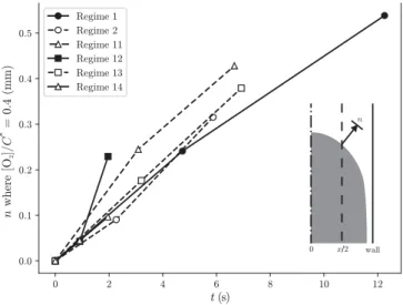
Fig. 11. Evolution of the [ O 2 ] /C ∗= 0 . 4 layer thickness normal to the bubble inter- face.

Fortheseregimes,itcanbeobservedinFig.11thatthe bound-ary layers evolve almost linearly over time, or even faster for regime 12,whichreflects theenhancementoftransfer duetothe recirculation patternsin theslugscompared to apurely diffusive case,whichwouldcorrespondtoanevolutionasthesquarerootof time. Surprisingly,it canbe seeninFig.11that comparablerates of evolution of theselayer thicknesses atthese points are found forallregimes,despitedifferentmagnitudesofrecirculation veloc-ities intheslugs.The impactoftheserecirculationvelocitieswill be morenoticeably visiblewhen analysing the averageslug con-centrationdynamics.

Nowtheexaminationoftemporalevolutionofradial concentra-tionprofilesbothbehindthebubbleandatmid-lengthoftheslug emphasestherole ofthefilmalongthechannelwall inthemass transfer process. Asa reminder, the filmregion formasstransfer analysisisdefinedall alongthechannel wall:next tothebubble, itcorrespondstothelubricationfilmandintheslugarea,itisthe region lying between the radial position of the dividing stream-line r1 andthe channel wall. Among all cases considered in this

section,twoconfigurationscanbedistinguishedbasedonthe con-centration profileinthefilm: thisisillustrated inFig.12 by pre-sentingtheradial profilesrecordedattimest1 andt2 forregimes

1and14.Regime1isrepresentativeofacaseofathinlubrication film (smallCa) likeregimes2,11and13,whereasregime 14 cor-respondstoathickerfilm(higherCa)whichhasdynamicssimilar toregime12.

Inthecaseofregime1,thefilmistheregionthemost concen-trated inO2,showingaconcentration levelevenhigherthanthat

observed intheslugregionnext tothe axisofsymmetry(x₌0). The maximumconcentration area seems to be close to thewall, underthelimitoftheresolutionoftheexperimental setupinthe filmregion(probablyinsufficientatt1 becausethethinzonewith

a zeroconcentration gradientatthewallis notvisibleatthis in-stant, contrary tot2), which leadstothe beliefthat thefirst and

majorsourceofoxygencorrespondstoazonewheretheinterface is theclosest tothe wall,atthe pointwhere thelubricationfilm thicknessshouldbetheminimum.Then,thefilmbecomesrapidly saturated inO2 witha clearhomogenisation inconcentration

be-tween positions z1 and z2, due to the combination of rapid

dif-fusion through the thinfilm adjacentto the bubbleand efficient convective transport bythe slidingvelocitybetweenthefilm and the bubble. Consequently,for thiscase, the filmrapidly becomes another source ofO2 forthe slugregion,in additionto the

bub-Fig. 12. Radial profiles of [O 2 ]/ C ∗in the centre of the slug from x = 0 to 1.5 mm with the corresponding concentration field inset.

ble interface directly in contactwith theslug. Inparticular, data extractedfromtheconcentrationprofilesofFig.12show thatthe concentrationgradientintheradialdirectionatthepositionofthe dividing streamline – whichrepresents the rate ofmass transfer betweenthe filmandthecentreofthe slug– is10 timeshigher than thecorrespondingradial gradientobservedinthevicinityof thesymmetryaxis– whichrepresentstherateofmasstransfer be-tweentheregionneartheaxisandthecentreoftheslug.For mod-elling purposes, if one decides to separate the whole liquidinto a slugregion and afilm region, it isthus compulsory to include a rateof mass transfer between the film and slug(Butleret al., 2016).

Inthecaseofregime 14(seeFig.12(c)and(d)),accessto ear-lier stages ofthe masstransfer dynamics ispossible becausethe diffusionprocessisslowercomparedtoregimes1and2duetoa lower diffusioncoefficient inthewater-Breoxsolutions. Notethat concentrationprofileveryclosetothewallisagainnottotallywell capturedatt1 becausethezerogradientareaoftheconcentration

fieldatthewallisnotaccuratelydescribed.Howeverthehigh res-olutionofthistechniqueassociatedwithalargelubricationfilmin thiscaseallowsustoobtainasufficientlygooddescriptionofthe concentration field inthe film. It can be observed that the pro-fileistotallydifferenttothepreviouscasesinceitpresentsalocal maximumatthepositionofthedividingstreamline,corresponding therefore to a filament ofdissolved O2 coming from the bubble,

visiblein Fig.12(c). This filamentfeeds both theslug regionand therestofthefilm,withcomparableratesofmasstransferateach sideofr1.Contrarytothepreviouscase,thefilmisvery

heteroge-neousinconcentration witha non-monotonousprofileinthe ra-dialdirection,andwenoticeforinstantt2(seeFig.12(c))the

pres-enceofanotherlocalmaximumclosetothewall,whichraisesthe questionofanadditionalsourceofO2diffusioncomingfroman

in-terfacepointveryclosetothewall. Thesetwo sourcescontribute totheincreaseinthefilmconcentrationovertime.Therefore,the dynamicsinthefilmare morecomplexfortheseregions oflarge

Ca and low mass diffusivity (14 and 12). Finally, the two differ-entdynamicsobservedhereconcerningtheroleplayedbythefilm inthetransferdynamicsoriginatefromdifferentfilm thicknesses, butalsoprobablyfromlocaldifferencesofcurvaturesofthe bub-bleshapes.It couldthen be informativetocompletethese obser-vationsthrough numericalstudies thatcould provide evidenceof the feeding points for the diffusionprocess andthe influence of interfaceshapes.

Toprovideguidancefortheestimationofthemasstransfer be-tween thefilm andslug areas,thediffusive rate hasbeen calcu-latedfromthePLIF-Iconcentrationfieldsby

ϕ

f ilm−s=−D

· ∂

[O2]

∂

x

¸

x=r1 (7)

Fig. 13. Local Sherwood number for the estimation of the mass transfer rate be- tween film and slug, determined at instants t 1 and t 2 for regimes 1, 2, and 11–14.

andalocalSherwoodnumberhasbeendefinedas

Shf ilm−s=

d[

∂

[O2]/

∂

x]x=r1

C∗ (8)

Fig.13 showsShf ilm−smeasured atthetwo instantst1 andt2 for

these six regimes asa function of the Peclet number Peb=uDbd,

definedbyusingtheslidingvelocityinthelubricationfilm,which isclosetou_b.Itis observedthatthislocalSherwoodnumber re-mainsnearlyconstant,rangingfrom10to20,andpresentsavery lowdependencyonPebeventhoughthelattervariesbymorethan

oneorderofmagnitude.

4.6. TransitiontoregimesatRe_b>300

Withvalues ofReb>300,which is thecase forregimes3–10,

other featuresappearintheconcentrationfieldswhichcannot be explained by a dynamic similar to what has been described at lowerReb.Thistransitionoccursbetweenregimes2and3.In

par-ticular,thepresenceoflocalmaximaofconcentrationinthecentre oftheslug,suchasinregime3,canbeobservedandsome coher-entstructuresofspecificconcentrationlevelsareclearlyvisiblefor regimes4–10. As a reminder, thesestructuresare also visibleon the instantaneousPLIF-I images.To ourknowledge, such features inconcentrationfieldshavenotbeenreportedinliterature sofar, neitherinexperimentalnorinnumericalworks.

Several hypotheses can be claimed to explain these observa-tions.Firstly,thisphenomenon couldoriginatefromparticular hy-drodynamics close to the T-mixer, in a similar wayto what was observedby Yangetal.(2016)who foundthat theinjectionzone isresponsibleforasignificantproportionoftheoverallmass trans-fer.Moreover, thestructuresofconcentrationcontours, whichare visible on the average fields for regimes at Reb>300, also lead

to the belief that a flow instability could appear at sufficiently high Reb and produce vortices in the slug and/or fluctuationsof

low intensity. Such an instability may come up in the bubble wake duetothe presenceof impuritieslike surfactantsadsorbed at the bubble surface, therefore giving a solid-like behaviour to theinterface atthe rearoftheTaylorbubble.Indeed,itisknown that in the caseof an unconfined flow past a solid particle, the sphere wakeremains steadyandaxisymmetric provided that the Reynoldsnumberislowerthan200.Abovethisvaluehowever, ax-isymmetry firstvanishes for Reynoldsnumbers between210 and 270, and unsteady flows are observed for larger Reynolds num-bers (Johnson and Pattel, 1999). Thus, wake instability in such

a flow appears at Reynolds numbers comparableto the value of 300that isobserved heretobe criticalin (confined)Taylorflow, whichsupports thisassumptionoftheresultofinterface contam-ination.Todateandtothebestofour knowledge,theonlywork wherea Taylorflow image ofthe concentration field isvisible is Kastensetal.(2017)whereasingleTaylorbubbleisstudiedbythe PLIF-ItechniqueforShintherange200–2000.Theysuggest surfac-tantsasa possiblecauseto anomalous concentrationdistribution andhighlightthefactthat,inthistypeofexperiment, aperfectly cleansystemisnearlyimpossibletoachieve underrealistic condi-tions.

On the PIV images of the present work, even if non-axisymmetric features are not observed in the slug when

Reb>300,thePIVmeasurementsrevealflowunsteadiness.Around

thecriticalvalueforReb,forthetwoflow regimes2and3,

char-acterised,respectively, by Reb=260 and Reb=400, the

fluctuat-ingvelocity fieldshavebeencalculated. Fig.14(a)showsthat ve-locityfluctuationsalongthe axisofsymmetry atx₌0reach sev-eral percents of the bubble velocity. We precise that the uncer-tainty ofthe velocity fluctuationshave beenquantified following Sciacchitanoand Wieneke(2016), andremains much lower than theobservedfluctuations, intherangeof0.2%ofub.Higher

fluc-tuationscanbenoticedintheaxialregionforregime3compared toregime 2,withmaximumvalueslocalised neartherearof the bubble.Thesefluctuationsdecreaseinintensityupto thenoseof thefollowing bubble.Thisobservationtends to confirmthe exis-tenceofaninstabilityproducedinthebubblewake,andassociated withfluctuations of about 4% of ub (for regime 3), even though

thevelocity field issued fromPIV analysis forregime 3 doesnot reveal any coherent structure in the bubble wake. Subsequently, consequencesarevisibleonthe masstransferdynamicsforthese regimes.Ifwecomparethemeanconcentrationfieldsofregimes2 and3inFig.9,focusingclosetotheaxisbetweenthebubblenose andtail,we noticea thinzone of highconcentration forregime 2,whichisricherthanthatobservedinregime3,thelatterbeing alsowider inthe axial region.Byfurther comparing the longitu-dinalconcentration profilesalong the axisinFig. 14(b),regime 2 exhibitssymmetry ofthe concentration profile,witha horizontal axispassinghalfwaythroughtheslug,whileforregime3, symme-tryisbroken andO2 concentration isincreasing fromtherear of

thebubbletothenoseofthefollowingone.Inthislattercase,this suggeststhatthevelocityfluctuationsclosetotherearofthe bub-bleenhancemixingandmodifythetopologyoftheconcentration field compared to stableregimes atReb<300. Forregimes 4–10,

thestructureoftheconcentrationfieldintheslugismodifiedeven furtherthanthatofregime3.

Note that, for all these disturbed regimes, the concentration field inthe film region doesnot show spatial heterogeneities, as comparedtothose observedinthe slug. Thefilm isalways more concentratedthattherestoftheslug,meaningitremains,aswell asthebubbleinterface,asourceofO2 thatfeedstheinnerslug.

Inthefollowingsection,despitethepresenceofperturbed pat-ternsofconcentrationintheslugsforregimes3–10duetoa pos-siblewakeinstability,anattempttorelatetheglobalmasstransfer dynamicstothe intensityoftherecirculationmotion intheslug, forallthestudiedregimes,isperformed.

4.7.Globalmasstransferdynamicsandscalinglaw

4.7.1. Masstransferdynamics

For allregimes, 4valuesof localnormalised liquid concentra-tionC(z)/C∗ _{areknown: thevaluesatinletandoutletofthetube}

sectionweremeasured bytheO2sensor, andthevaluesobtained

byspatial averagingofthelocalconcentrationfieldfromthe PLIF-Iimagesacquired atthe two axial positions z1 andz2.Theycan

Fig. 14. Axial profiles at x = 0 for regimes 2 and 3 (a) relative bubble velocity fluctuation, (b) normalised oxygen concentration.

cell C(t)/C∗_{by usingthebubbleresidencetime,definedast=} z u_b.

Fromthefourmeasuredpoints,themasstransferdynamicscanbe quantified. It is noted herethat the notation forconcentration C

differsfrom[O2]usedpreviously,asthelatterreferstotheoxygen

concentration valuesin the concentration field, while theformer referstothevolumetricaverageoxygenconcentrationintheliquid phase,calculatedinamannersimilartoEq.(3).

ThesimplestmodelbasedononeglobaltransfercoefficientkL,

assumed constant,writes theinstantaneous rateof masstransfer as

ϕ

uc

(

t

)

=Voluc dC dt =kLaVoluc[C ∗ − C

(

t

)

] (9)

where a is the gas–liquid interfacial area per unit cell volume which isknown foreach regime fromprocessingofthe shadow-graphimages.ThesolutionofEq.(9)predictsatemporalevolution intheform

C

(

t

)

/C∗

=1_{− e}−kLa t ₍₁₀₎

Thismodelisreferredtoastheplugflowmodel,correspondingto anassumptionofuniformityofvelocityandconcentrationineach unit cell of the Taylor flow, and it is associated to the volumet-ric masstransfercoefficient kLa.Fig.15 comparesthe

experimen-tal measurementsforeachregime withthismodelwherethekLa

valueshavebeenchosenbyleast-squaresfitting.Itshowsthatthe plugflowpredictionquiteaccuratelydescribesthetransfer dynam-icsformostregimes,withtheworstfitsbeingregimes4,5,11and 13 forwhichthedynamics areslightlyunderestimated. Forthese cases, aglobal 1stordermodel cannot accurately predict the ac-tualdecreaseofmasstransferratebetweenthetwophaseswhich isobservedaftera certaintime (Butleretal., 2016). Nevertheless, it can be considered sufficient,as afirst approximation, to usea modelwithoneadjustableparameterkL becauseonlyfour

instan-taneousexperimentalvaluesofconcentrationareavailableforeach regime.NotethatkLa valuereachesupto2.46s−1,associatedtoa

Sherwoodnumberof4000(regime8).

4.7.2. ScalinglawfortheoverallmasstransferinTaylorflow

Thetransferdynamicscanthen becomparedbetweenthe dif-ferentregimesbydefiningaglobalSherwoodnumberasSh₌ kLd

D .

Apriori,themasstransferdynamicscoulddependonthe

indepen-dentnon-dimensionalnumbersoftheproblem,i.e.(Reb,Sc,We).In

theconcentrationfields,thefilmzonerepresentsavolumeofonly 10%ofVoluc atmaximum(incasesoflargerlubricationfilms).The

evolution of the average liquidconcentration is therefore mainly controlled by the concentration reached in the slug, keeping in mindtheroleofthefilminthetransferprocessasa complemen-tarysourceofdissolvedO2fortheslug.Intheslug,ifweassumea

Poiseuilleflow, withoutconsideringthe presenceofanytemporal fluctuations,thevelocitywhichensuresmasstransfercorresponds tothevelocityoftheliquidrelativetothebubble,nomatterifthe Taylorflowisascendingordescending,withaprofilegivenby

u

(

x

)

=2ut p

·

1_{− 4}

³

x d

´

2

¸

− ub (11)

This profile describes a recirculation motion in the slug, with a radial position r0=₂√d₂

q

2₋ ub

u_{t p} where velocity vanishes (see

Fig.10). From this,following Thulasidas etal.(1997),the average recirculationvelocityinthevortexcanbecalculatedbasedonthe time t_cir required to displace liquid from the rear of one bubble tothe noseof thefollowing one inthe train (i.e.along one slug lengthLs), ucir= Ls tcir (12) with tcir=

π

Lsr20 2

π

Rr0 0 u

(

x

)

xdx = Ls 2ut p− 4ut p

¡

r_d0

¢

2 − ub (13) Finally,therecirculationvelocityinthecapillarytubeisgivenby

ucir=2ut p− 4ut p

³

_r0

d

´

2

− ub (14)

Notethat, using the expressionof r0,it can be found that ucir= ut p−12ub. From Eq.(14),a recirculationReynoldsnumber can be

definedasRecir=ρL_µucir_Ld.Recir isexpected tohave a strong

influ-enceonthemasstransferbecause,intheslug,diffusionisensured across the streamlines of the recirculation motion, with sources of O2 coming from (i) the nearly spherical rear of a bubble, (ii)

thenearlysphericalnoseofthefollowingbubbleand(iii)thefilm whichismoreconcentratedthantheslug.

Ata givenvalue ofSchmidt number,i.e. forall waterregimes 1to10 atSc₌526,Shasa functionofRecir isplottedinFig.16.

Fig. 15 . Evolution of C ( t )/ C ∗ _{in the overall liquid phase (slug + film) along the channel (as t =} z

ub) for all regimes showing the experimental points and the fitted plug flow model of Eq. (10) .

Fig. 16. Re cir vs Sh for all water regimes at Sc = 526 .

Itcanbe seenthatall pointslie onasinglecurve,demonstrating theimportance ofthe intensityoftherecirculationmotioninthe transfer dynamics.Thisslightdiscrepancyof thispowerlawmay resultfromthelarge variationsofWe(overtwoorders of magni-tude) forall theseregimes;however,Recir isclearlythe most

im-portantparameterwhichgivesShatagivenSc.

With the objective to produce a simple predictive correlation for the mass transfer coefficient for all regimes studied in the present article, which relies on an interpretation of the transfer dynamics by a plug flow model withconstant mass transfer co-efficient,the choice is madeto consider asa first approximation that ub≈ utp,whichresultsin Recir≈12Reb. Itis thenproposed to

relate Sh asa function of both Reb andSc. In thisway, the final

scalinglawisthen

Sh₌1.051_{× 10}−6_Re1.895

b Sc

1.331 ₍₁₅₎

Fig. 17. Comparison of Eq. (15) to available scaling laws from literature.

Table 3

Scaling laws from literature chosen as reference for the present work. Reference Correlation

Ber ˇci ˇc and Pintar (1997) Sh = d aD 0 . 111 u1.19 t p [(1−εg)Luc]0.57 q D DCH4

Van Baten and Krishna (2004) Sh = d aD µ 2√2 π q Dub d 4 Luc+ 2 √_π q Dub εgLuc 4εg d ¶ Vandu et al. (2005) Sh = d aD 4 . 5 q Dugs Luc 1 d

Note that exponent of Reb is nearly the same as that of Recir in

the powerlawfunctionin Fig.16,andthatthe useofWeinthis proposedcorrelationdoesnothelpinimprovingitsaccuracy.

This scaling law is compared in Fig. 17 to well known scal-ing laws available in literature (see Table 3) which are