HAL Id: inria-00541865
https://hal.inria.fr/inria-00541865
Submitted on 27 Jan 2011
HAL is a multi-disciplinary open access
archive for the deposit and dissemination of
sci-entific research documents, whether they are
pub-lished or not. The documents may come from
teaching and research institutions in France or
abroad, or from public or private research centers.
L’archive ouverte pluridisciplinaire HAL, est
destinée au dépôt et à la diffusion de documents
scientifiques de niveau recherche, publiés ou non,
émanant des établissements d’enseignement et de
recherche français ou étrangers, des laboratoires
publics ou privés.
using a full-rank spatial covariance model
Ngoc Duong, Emmanuel Vincent, Rémi Gribonval
To cite this version:
Ngoc Duong, Emmanuel Vincent, Rémi Gribonval.
Under-determined reverberant audio source
separation using a full-rank spatial covariance model. IEEE Transactions on Audio, Speech and
Language Processing, Institute of Electrical and Electronics Engineers, 2010, 18 (7), pp.1830–1840.
�10.1109/TASL.2010.2050716�. �inria-00541865�
Under-determined reverberant audio source
separation using a full-rank spatial covariance model
Ngoc Q. K. Duong, Emmanuel Vincent and R´emi Gribonval
Abstract—This article addresses the modeling of reverberant
recording environments in the context of under-determined convolutive blind source separation. We model the contribution of each source to all mixture channels in the time-frequency domain as a zero-mean Gaussian random variable whose covari-ance encodes the spatial characteristics of the source. We then consider four specific covariance models, including a full-rank unconstrained model. We derive a family of iterative expectation-maximization (EM) algorithms to estimate the parameters of each model and propose suitable procedures adapted from the state-of-the-art to initialize the parameters and to align the order of the estimated sources across all frequency bins. Experimental results over reverberant synthetic mixtures and live recordings of speech data show the effectiveness of the proposed approach.
Index Terms—Convolutive blind source separation,
under-determined mixtures, spatial covariance models, EM algorithm, permutation problem.
I. INTRODUCTION
In blind source separation (BSS), audio signals are generally mixtures of several sound sources such as speech, music, and background noise. The recorded multichannel signal x(t) is therefore expressed as x(t) = J ! j=1 cj(t) (1)
where cj(t) = [c1j(t), ..., cIj(t)]T is the spatial image of the
jth source, that is the contribution of this source to all mixture channels,I is number of mixture channels. For a point source in a reverberant environment, cj(t) can be expressed via the
convolutive mixing process cj(t) =!
τ
hj(τ )sj(t − τ) (2) where sj(t) is the jth source signal and hj(τ ) =
[h1j(τ ), ..., hIj(τ )]T the vector of filter coefficients modeling
the acoustic path from this source to all microphones. Source separation consists in recovering either the J original source signals or their spatial images given theI mixture channels. In the following, we focus on the separation of under-determined mixtures, i.e. such thatI < J, assuming that J is known.
Most existing approaches operate in the time-frequency domain using the short-time Fourier transform (STFT) and rely on narrowband approximation of the convolutive mixture
Manuscript received November 22, 2009.
The authors are with INRIA, Centre Inria Rennes - Bretagne Atlantique, 35042 Rennes Cedex, France (e-mail: [email protected]; [email protected]; [email protected]).
Part of this work has been presented at the 2010 IEEE International Confer-ence on Acoustics, Speech and Signal Processing [1].
(2) by complex-valued multiplication in each frequency binf and time frame n as
cj(n, f ) ≈ hj(f )sj(n, f ) (3) where theI × 1 mixing vector hj(f ) is the Fourier transform
of hj(τ ), sj(n, f ) are the STFT coefficients of the sources
sj(t) and cj(n, f ) = [c1j(n, f ), ..., cIj(n, f )]T the STFT
coefficients of their spatial images cj(t). The sources are
typically estimated under the assumption that they are sparse in the STFT domain. For instance, the degenerate unmixing es-timation technique (DUET) [2] uses binary masking to extract the predominant source in each time-frequency bin. Another popular technique known as "1-norm minimization extracts
on the order ofI sources per time-frequency bin by solving a constrained"1-minimization problem [3], [4]. The separation
performance achievable by these techniques remains limited in reverberant environments [5], due in particular to the fact that the narrowband approximation does not hold because the mixing filters are much longer than the window length of the STFT.
Recently, a distinct framework has emerged whereby the STFT coefficients of the source images cj(n, f ) are
mod-eled by a phase-invariant multivariate distribution whose pa-rameters are functions of (n, f ) [6]. One instance of this framework consists in modeling cj(n, f ) as a zero-mean
Gaussian random variable with covariance matrix Rcj(n, f ) =
E(cj(n, f )cHj (n, f )) factored as
Rcj(n, f ) = vj(n, f ) Rj(f ) (4)
where vj(n, f ) are scalar time-varying variances encoding
the spectro-temporal power of the sources and Rj(f ) are
I ×I time-invariant spatial covariance matrices encoding their spatial position and spatial spread [7]. The model parameters can then be estimated in the maximum likelihood (ML) sense and used to estimate the spatial images of all sources by Wiener filtering.
This framework was first applied to the separation of instantaneous audio mixtures in [8], [9] and shown to provide better separation performance than"1-norm minimization. The
instantaneous mixing process then translated into a rank-1 spatial covariance matrix for each source. In our preliminary paper [7], we extended this approach to convolutive mixtures and proposed to consider full-rank spatial covariance matrices modeling the spatial spread of the sources and circumvent-ing the narrowband approximation to a certain extent. This approach was shown to improve separation performance of reverberant mixtures in both an oracle context, where all model parameters are known, and in a semi-blind context,
where the spatial covariance matrices of all sources are known but their variances are blindly estimated from the mixture.
In [1] and the following, we extend this work to blind esti-mation of the model parameters as required for realistic BSS application. This article provides three main contributions. Firstly, we explain the appropriateness of full-rank spatial co-variance models in the context of reverberant source separation and propose a new full-rank unconstrained model. Secondly, we design parameter estimation algorithms for these models by deriving the corresponding expectation-maximization (EM) [10] update rules and adapting the sparsity-based algorithms in [3], [11] for parameter initialization and permutation align-ment. Thirdly, we show that the proposed full-rank uncon-strained model outperforms state-of-the-art algorithms on a wide range of data and estimation scenarios.
The structure of the rest of the article is as follows. We introduce the general framework under study as well as four specific spatial covariance models in Section II. We then address the blind estimation of all model parameters from the observed mixture in Section III. We compare the source separation performance achieved by each model to that of state-of-the-art techniques in various experimental settings in Section IV. Finally we conclude and discuss further research directions in Section V.
II. GENERAL FRAMEWORK AND SPATIAL COVARIANCE MODELS
We start by describing the general probabilistic modeling framework adopted from now on. We then define four models with different degrees of flexibility resulting in rank-1 or full-rank spatial covariance matrices.
A. General framework
Let us assume that the vector cj(n, f ) of STFT coefficients
of the spatial image of the jth source follows a zero-mean Gaussian distribution whose covariance matrix factors as in (4). Under the classical assumption that the sources are uncor-related, the vector x(n, f ) of STFT coefficients of the mixture signal is also zero-mean Gaussian with covariance matrix
Rx(n, f ) = J
!
j=1
vj(n, f ) Rj(f ). (5)
In other words, the likelihood of the set of observed mixture STFT coefficients x= {x(n, f)}n,f given the set of variance
parametersv = {vj(n, f )}j,n,f and that of spatial covariance
matrices R= {Rj(f )}j,f is given by P (x|v, R) =" n,f 1 det (πRx(n, f )) e−xH(n,f )R−1 x (n,f )x(n,f ) (6) whereH denotes matrix conjugate transposition and Rx(n, f )
implicitly depends on v and R according to (5). In the fol-lowing, we assume that the source variances are unconstrained and focus on modeling the covariance matrices by higher-level spatial parameters.
Under this model, source separation can be achieved in two steps. The variance parameters v and the spatial parameters
underlying R are first estimated in the ML sense. The spatial images of all sources are then obtained in the minimum mean square error (MMSE) sense by multichannel Wiener filtering #cj(n, f ) = vj(n, f )Rj(f )R−1x (n, f )x(n, f ). (7)
B. Rank-1 convolutive model
Most existing approaches to audio source separation rely on narrowband approximation of the convolutive mixing process (2) by the complex-valued multiplication (3). The covariance matrix of cj(n, f ) is then given by (4) where vj(n, f ) is the
variance ofsj(n, f ) and Rj(f ) is equal to the rank-1 matrix
Rj(f ) = hj(f )hHj (f ) (8) with hj(f ) denoting the Fourier transform of the mixing filters
hj(τ ). This rank-1 convolutive model of the spatial covariance matrices has recently been exploited in [12] together with a different model of the source variances.
C. Rank-1 anechoic model
For omni-directional microphones in an anechoic recording environment without reverberation, each mixing filter boils down to the combination of a delayτij and a gainκijspecified
by the distancerij from thejth source to the ith microphone
[13] τij= rij c and κij = 1 √ 4πrij (9) where c is sound velocity. The spatial covariance matrix of thejth source is hence given by the rank-1 anechoic model
Rj(f ) = aj(f )aHj (f ) (10) where the Fourier transform aj(f ) of the mixing filters is now
parameterized as aj(f ) = κ1,je−2iπf τ1,j .. . κI,je−2iπf τI,j
. (11)
D. Full-rank direct+diffuse model
One possible interpretation of the narrowband approxima-tion is that the sound of each source as recorded on the micro-phones comes from a single spatial position at each frequency f , as specified by hj(f ) or aj(f ). This approximation is not
valid in a reverberant environment, since reverberation induces some spatial spread of each source, due to echoes at many different positions on the walls of the recording room. This spread translates into full-rank spatial covariance matrices.
The theory of statistical room acoustics assumes that the spatial image of each source is composed of two uncorrelated parts: a direct part, which is modeled by aj(f ) in (11) for
omni-directional microphones, and a reverberant part. The spatial covariance Rj(f ) of each source is then a full-rank
matrix defined as the sum of the covariance of its direct part and the covariance of its reverberant part such that
Rj(f ) = aj(f )aHj (f ) + σ2
whereσ2
rev is the variance of the reverberant part andΨil(f )
is a function of the distance dil between the ith and the lth
microphone such thatΨii(f ) = 1. This model assumes that the
reverberation recorded at all microphones has the same power but is correlated as characterized by Ψil(f ). This model has
been employed for single source localization in [13] but not for source separation yet.
Assuming that the reverberant part is diffuse, i.e. its inten-sity is uniformly distributed over all possible directions, its normalized cross-correlation can be shown to be real-valued and equal to [14]
Ψil(f ) =
sin(2πf dil/c)
2πf dil/c
. (13) Moreover, the power of the reverberant part within a paral-lelepipedic room with dimensions Lx,Ly,Lz is given by
σrev2 =
4β2
A(1 − β2) (14)
where A is the total wall area and β the wall reflection coefficient computed from the room reverberation time T60
via Eyring’s formula [13] β = exp * − 13.82 (L1x +L1y +L1z)cT60 + . (15)
Note that the covariance matrix Ψ(f ) is usually employed for the modeling of diffuse background noise. For instance, the source separation algorithm in [15] assumes that the sources follow an anechoic model and represents the non-direct part of all sources by a shared diffuse noise component with covariance Ψ(f ) and constant variance. Hence this algorithm does not account for correlation between the variances of the direct part and the non-direct part. On the contrary, the direct+diffuse model scales the direct and non-direct part of Rj(f ) by the same variance vj(n, f ), which is more consistent with the physics of sound.
E. Full-rank unconstrained model
In practice, the assumption that the reverberant part is dif-fuse is rarely satisfied in realistically reverberant environments. Indeed, early echoes accounting for most of its energy are not uniformly distributed on the boundaries of the recording room. When performing some simulations in a rectangular room, we observed that (13) is valid on average when considering a large number of sources distributed at different positions in a room, but generally not valid for each individual source.
Therefore, we also investigate the modeling of each source via a full-rank unconstrained spatial covariance matrix Rj(f )
whose coefficients are unrelated a priori. This model is the most general possible model for a covariance matrix. It gen-eralizes the above three models in the sense that any matrix taking the form of (8), (10) or (12) can also be considered as an unconstrained matrix. Because of this increased flexibility, this unconstrained model better fits the data as measured by the likelihood. In particular, it improves the poor fit between the model and the data observed for rank-1 models due to the fact that the narrowband approximation underlying these
models does not hold for reverberant mixtures. In that sense, it circumvents the narrowband approximation to a certain extent. The entries of Rj(f ) are not directly interpretable in terms
of simple geometrical quantities. The principal component of the matrix can be interpreted as a beamformer [16] pointing towards the direction of maximum output power, while the ratio between its largest eigenvalue and its trace is equal to the ratio between the output and input power of that beamformer. In moderate reverberation conditions, the former is expected to be close to the source direction of arrival (DOA) while the latter is related to the ratio between the power of direct sound and that of reverberation. However, the strength of this model is precisely that it remains valid to a certain extent in more reverberant environments, since it is the most general possible model for a covariance matrix.
III. BLIND ESTIMATION OF THE MODEL PARAMETERS
In order to use the above models for BSS, we need to estimate their parameters from the mixture signal only. In our preliminary paper [7], we used a quasi-Newton algorithm for semi-blind separation that converged in a very small number of iterations. However, due to the complexity of each iteration, we later found out that the EM algorithm, which is a popular choice for Gaussian models [15], [17], [18], provided faster convergence despite a larger number of iterations.
As any iterative optimization algorithm, EM is sensitive to initialization [12] so that a suitable parameter initialization scheme is necessary. Also, the well-known source permutation problem must be addressed when the model parameters are in-dependently estimated at different frequencies [11]. We hence adopt the following three-step procedure as depicted in Fig. 1: initialization of hj(f ) or Rj(f ) by hierarchical clustering,
iterative ML estimation of all model parameters via EM, and direction of arrival (DOA) based permutation alignment. The latter step is needed only for the rank-1 convolutive model and the full-rank unconstrained model whose parameters are estimated independently in each frequency bin. It is conducted after EM parameter estimation, since optimized parameters provide better DOA information than initial ones and EM does not always preserve the order of the sources.
Fig. 1. Flow of the proposed blind source separation approach.
A. Initialization by hierarchical clustering
Preliminary experiments showed that the initialization of the model parameters greatly affects the separation performance
resulting from the EM algorithm. Yet, the parameter initializa-tion schemes previously proposed for rank-1 Gaussian models are either restricted to instantaneous mixtures [18] or non-blind [7], [12]. By contrast, a number of clustering algorithms have been proposed for blind estimation of the mixing vectors in the context of sparsity-based convolutive source separation. In the following, we use up to minor improvements the hierarchical clustering-based algorithm in [3] for the purpose of parameter initialization of rank-1 models and introduce a modified version of this algorithm for parameter initialization of full-rank models.
The algorithm in [3] relies on the assumptions that at each frequency f the sounds of all sources come from disjoint regions of space and that a single source predominates in most time-frequency bins. The vectors x(n, f ) of mixture STFT coefficients then cluster around the direction of the associated mixing vector hj(f ) in the time frames n where the jth source
is predominant. It is well known that the validity of the latter sparsity assumption decreases with increasing reverberation. Nevertheless, this algorithm was explicitly developed for re-verberant mixtures.
In order to estimate these clusters, the vectors of mixture STFT coefficients are first normalized as
¯
x(n, f ) ← x(n, f ) &x(n, f)&2
e−iarg(x1(n,f ))
(16) where arg(.) denotes the phase of a complex number and &.&2the Euclidean norm. We then define the distance between
two clusters C1 andC2 by the average distance between the
associated normalized mixture STFT coefficients d(C1, C2) = 1 |C1||C2| ! ¯ xc1∈C1 ! ¯ xc2∈C2 &¯xc1− ¯xc2&2 (17)
In a given frequency bin f , each normalized vector of mixture STFT coefficients ¯x(n, f ) at a time frame n is first considered as a cluster containing a single item. The distance between each pair of clusters is computed and the two clusters with the smallest distance are merged. This ”bottom up” process called linking is repeated until the number of clusters is smaller than a predetermined threshold K. This threshold is usually much larger than the number of sources J [3], so as to eliminate outliers. We finally choose theJ clusters with the largest number of samples and compute the initial mixing vector and spatial covariance matrix for each source as
hinitj (f ) = 1 |Cj| ! ¯ x(n,f )∈Cj ˜ x(n, f ) (18) Rinitj (f ) = 1 |Cj| ! ¯ x(n,f )∈Cj ˜ x(n, f )˜x(n, f )H (19)
where ˜x(n, f ) = x(n, f )e−iarg(x1(n,f )), and|C
j| denotes the
total number of samples in clusterCj, which depends on the
considered frequency binf .
Note that, contrary to the algorithm in [3], we define the distance between clusters as the average distance between the normalized mixture STFT coefficients instead of the minimum distance between them. Besides, the mixing vector hinitj (f )
is computed from the phase-normalized mixture STFT coef-ficients ˜x(n, f ) instead of both phase and amplitute normal-ized coefficients ¯x(n, f ). This increases the weight of time-frequency bins of large amplitude where the modeled source is more likely to be prominent, in a way similar to [2]. These modifications were found to provide better initial approxima-tion of the mixing parameters in our experiments. We also tested random initialization and DOA-based initialization, i.e. where the mixing vectors hinitj (f ) are derived from known
source and microphone positions assuming no reverberation. Both schemes were found to result in slower convergence and poorer separation performance than the chosen scheme.
The source variances were initialized to vinit
j (n, f ) = 1.
This basic initialization scheme did not significantly affect per-formance compared to the slower advanced scheme consisting of finding the vinit
j (n, f ) most consistent with hinitj (f ) and
Rinitj (f ) by running EM without updating the mixing vectors or the spatial covariance matrices.
B. EM updates for the rank-1 convolutive model
The derivation of the EM parameter estimation algorithm for the rank-1 convolutive model is strongly inspired from the study in [12]. Indeed it relies on the same model of spatial covariance matrices but on a distinct unconstrained model of the source variances. Similarly to [12], EM cannot be directly applied to the mixture model (1) since the estimated mixing vectors remain fixed to their initial value. This issue can be addressed by considering the noisy mixture model
x(n, f ) = H(f )s(n, f ) + b(n, f ) (20) where H(f ) is the mixing matrix whose jth column is the mixing vector hj(f ), s(n, f ) is the vector of source STFT
coefficients sj(n, f ) and b(n, f ) some additive zero-mean
Gaussian noise. We denote by Rs(n, f ) the diagonal
covari-ance matrixof s(n, f ). Following [12], we assume that b(n, f ) is stationary and spatially uncorrelated and denote by Rb(f )
its time-invariant diagonal covariance matrix. This matrix is initialized to a small value related to the average empirical channel variance as discussed in [12].
EM is separately derived for each frequency bin f for the complete data {x(n, f), sj(n, f )}j,n that is the set of
observed mixture STFT coefficients and hidden source STFT coefficients of all time frames. The details of one iteration are as follows. In the E-step, the Wiener filter W(n, f ) and the conditional mean#s(n, f) and covariance #Rss(n, f ) of the
sources are computed as
Rs(n, f ) = diag(v1(n, f ), ..., vJ(n, f )) (21) Rx(n, f ) = H(f )Rs(n, f )HH(f ) + Rb(f ) (22) W(n, f ) = Rs(n, f )HH(f )R−1x (n, f ) (23) #s(n, f) = W(n, f)x(n, f) (24) # Rss(n, f ) = #s(n, f)#sH(n, f ) + (I − W(n, f)H(f))Rs(n, f ) (25) where I is theI × I identity matrix and diag(.) the diagonal matrix whose entries are given by its arguments. Conditional
expectations of multichannel statistics are also computed by averaging over all N time frames as
# Rss(f ) = 1 N N ! n=1 # Rss(n, f ) (26) # Rxs(f ) = 1 N N ! n=1 x(n, f )#sH(n, f ) (27) # Rxx(f ) = 1 N N ! n=1 x(n, f )xH(n, f ). (28)
In the M-step, the source variances, the mixing matrix and the noise covariance are updated via
vj(n, f ) = #Rssjj(n, f ) (29)
H(f ) = #Rxs(f ) #R−1ss(f ) (30)
Rb(f ) = Diag( #Rxx(f ) − H(f) #RHxs(f )
− #RxsHH(f ) + H(f ) #Rss(n, f )HH(f )) (31)
whereDiag(.) projects a matrix onto its diagonal.
C. EM updates for the full-rank unconstrained model
The derivation of EM for the full-rank unconstrained model is much easier since the above issue does not arise. We hence stick with the exact mixture model (1), which can be seen as an advantage of full-rank vs. rank-1 models. EM is again separately derived for each frequency binf . Since the mixture can be recovered from the spatial images of all sources, the complete data reduces to {cj(n, f )}n,f, that is the set of
hidden STFT coefficients of the spatial images of all sources on all time frames. The details of one iteration are as follows. In the E-step, the Wiener filter Wj(n, f ) and the conditional
mean #cj(n, f ) and covariance #Rcj(n, f ) of the spatial image
of the jth source are computed as
Wj(n, f ) = Rcj(n, f )R−1x (n, f ) (32)
#cj(n, f ) = Wj(n, f )x(n, f ) (33)
#
Rcj(n, f ) = #cj(n, f )#cHj (n, f ) + (I − Wj(n, f ))Rcj(n, f )
(34) where Rcj(n, f ) is defined in (4) and Rx(n, f ) in (5). In
the M-step, the variance and the spatial covariance of thejth source are updated via
vj(n, f ) = 1 Itr(R −1 j (f ) #Rcj(n, f )) (35) Rj(f ) = 1 N N ! n=1 1 vj(n, f ) # Rcj(n, f ) (36)
where tr(.) denotes the trace of a square matrix. Note that, strictly speaking, this algorithm is a generalized form of EM [19], since the M-step increases but does not maximize the likelihood of the complete data due to the interleaving of (35) and (36). The increase of the log-likelihood and of the separation performance resulting from these updates is illustrated in Section IV-C.
D. EM updates for the rank-1 anechoic model and the full-rank direct+diffuse model
The derivation of EM for the two remaining models is more complex since the M-step cannot be expressed in closed form. The complete data and the E-step for the rank-1 anechoic model and the full-rank direct+diffuse model are identical to those for the rank-1 convolutive model and the full-rank unconstrained model, respectively. The M-step, which consists of maximizing the likelihood of the complete data given their natural statistics computed in the E-step, could be addressed
e.g. via a quasi-Newton technique or by sampling possible parameter values from a grid [15]. In the following, we do not attempt to derive the details of these algorithms since these two models appear to provide lower performance than the rank-1 convolutive model and the full-rank unconstrained model in a semi-blind context, as discussed in Section IV-B.
E. Permutation alignment
Since the parameters of the rank-1 convolutive model and the full-rank unconstrained model, i.e. hj(f ), Rj(f ) and
vj(n, f ), are estimated independently in each frequency bin
f , they should be ordered so as to correspond to the same source across all frequency bins. This so-called permutation problem has ben widely studied in the context of sparsity-based source separation. In the following, we apply the DOA -based algorithm in [11] to the rank-1 model and explain how to adapt this algorithm to the full-rank model.
The principle of this algorithm is as follows. Given the geometry of the microphone array, a critical frequency is de-termined above which spatial aliasing may occur. The mixing vectors hj(f ) are each unambiguously related to a certain
DOA below that frequency while phase wrapping may occur at higher frequencies. The algorithm first estimates the source DOAs and the permutations at low frequencies by clustering the mixing vectors after suitable normalization assuming no phase wrapping and then re-estimates them at all frequencies by taking phase wrapping into account. Note that the order of source variances vj(n, f ) in each frequency bin is permuted
identically to that of the mixing vectors hj(f ).
Regarding the full-rank model, we first apply principal component analysis (PCA) to summarize the spatial covariance matrix Rj(f ) of each source in each frequency bin by its
first principal component wj(f ) that points to the direction of
maximum variance. This vector is conceptually equivalent to the mixing vector hj(f ) of the rank-1 model. Thus, we can
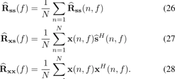
apply the same procedure to solve the permutation problem. Fig. 2 depicts the phase of the second entryw2j(f ) of wj(f )
before and after solving the permutation for a real-world stereo recording of three female speech sources with room reverberation time T60 = 250 ms, where wj(f ) has been
normalized as in (16). The critical frequency below which this phase is unambiguously related to the source DOAs is here equal to 5 kHz [11]. The source order appears globally aligned for most frequency bins after solving the permutation.
IV. EXPERIMENTAL EVALUATION
We evaluate the above models and algorithms under three different experimental settings. Firstly, we compare all four
Fig. 2. Normalized argument of w2j(f ) before and after permutation
align-ment from a real-world stereo recording of three sources withT60= 250 ms.
models in a semi-blind setting so as to estimate an upper bound of their separation performance. Based on these results, we select two models for further study, namely the rank-1 convolutive model and the full-rank unconstrained model. Secondly, we evaluate these models in a blind setting over synthetic reverberant speech mixtures and compare them to state-of-the-art algorithms over the real-world speech mixtures of the 2008 Signal Separation Evaluation Compaign (SiSEC 2008) [5]. Finally, we assess the robustness of these two models to source movements in a semi-blind setting.
A. Common parameter settings and performance criteria
The common parameter setting for all experiments are summarized in Table I. In order to evaluate the separation per-formance of the algorithms, we use the signal-to-distortion ra-tio (SDR), signal-to-interference rara-tio (SIR), signal-to-artifact ratio (SAR) and source image-to-spatial distortion ratio (ISR) criteria expressed in decibels (dB), as defined in [20]. These criteria account respectively for overall distortion of the target source, residual crosstalk from other sources, musical noise and spatial or filtering distortion of the target.
Signal duration 10 s Number of channels I= 2
Sampling rate 16 kHz Window type sine window STFT frame size 1024 STFT frame shift 512 Propagation velocity 343 m/s Number of EM iterations 10 Cluster threshold K= 30 TABLE I
COMMON EXPERIMENTAL PARAMETER SETTING
B. Potential source separation performance of all models
The first experiment is devoted to the investigation of the potential source separation performance achievable by each
model in a semi-blind context, i.e. assuming knowledge of the true spatial covariance matrices. We generated ten stereo synthetic mixtures of three speech sources, i.e. two mixtures with male voices only, two mixtures with female voices only, and six mixtures with mixed male and female voices, by convolving different sets of speech signals with room impulse responses simulated via the source image method. The positions of the sources and the microphones are illustrated in Fig. 3. The distance from each source to the center of the microphone pair was 120 cm and the microphone spacing was 20 cm. The reverberation time was set toT60= 250 ms.
Fig. 3. Room geometry setting for synthetic convolutive mixtures.
The true spatial covariance matrices Rj(f ) of all sources
were computed either from the positions of the sources and the microphones and other room parameters or from the mixing filters. More precisely, we used the equations in Sections II-B, II-C and II-D for rank-1 models and the full-rank di-rect+diffuse model and ML estimation from the spatial images of the true sources for the full-rank unconstrained model. The source variances were then estimated from the mixture using the quasi-Newton technique in [7], for which an efficient initialization exists when the spatial covariance matrices are fixed. Binary masking, "1-norm minimization and "0-norm
minimization were also evaluated for comparison using the reference software in [5]1 with the same mixing vectors as
for the rank-1 convolutive model. The SDR obtained with"1
-norm minimization was about 0.2 dB below that given by"0
-norm minimization, therefore only the latter is considered for comparison hereafter. The results are averaged over all sources and all set of mixtures and shown in Table II, together with the number of spatial parameters of each model, i.e. the number of parameters encoding the spatial characteristics of the sources. The rank-1 anechoic model has lowest performance in terms of SDR, SIR, and ISR because it only accounts for the direct path. By contrast, the full-rank unconstrained model has highest performance in terms of SDR and ISR. It improves the SDR by 1.7 dB, 1.2 dB, and 1.6 dB when compared to the rank-1 convolutive model, binary masking, and "0-norm
1Binary masking is achieved in each time-frequency bin by projecting the
mixture STFT coefficients x(n, f ) onto the subspace spanned by each mixing vector hj(f ) and selecting the source j0 whose projection has largest !2
norm. The spatial imagebcj
0(n, f ) of this source is then set to the projected
Covariance models
Number of spatial parameters
SDR SIR SAR ISR Rank-1 anechoic 6 0.9 2.4 7.8 5.1 Rank-1 convolutive 3078 4.0 7.9 5.4 9.5 Full-rank direct+diffuse 8 3.2 6.7 5.3 7.9 Full-rank unconstrained 6156 5.7 10.8 7.3 11.0 Binary masking 3078 4.5 10.1 5.0 9.4 !0-norm minimization 3078 4.1 7.7 5.9 9.5 TABLE II
AVERAGE POTENTIAL SOURCE SEPARATION PERFORMANCE IN A SEMI-BLIND SETTING OVER STEREO MIXTURES OF THREE SOURCES WITH
T60= 250MS.
minimization respectively. The full-rank direct+diffuse model results in a SDR decrease of 0.8 dB compared to the rank-1 convolutive model. This decrease appears surprisingly small when considering the fact that the former involves only 8 spatial parameters (6 distances rij, plus σrev2 and d) instead
of 3078 parameters (6 mixing coefficients per frequency bin) for the latter. Nevertheless, we focus on the two best models, namely the rank-1 convolutive model and the full-rank unconstrained model in subsequent experiments.
C. Blind source separation performance as a function of the reverberation time
The second experiment aims to investigate two things: firstly, the blind source separation performance achieved via these two models as well as via binary masking and "0-norm
minimization; and secondly, the convergence property of EM iterations for the proposed full-rank unconstrained model in different reverberant conditions. Ten synthetic speech mixtures were generated in the same as in the first experiment for each reverberant condition, except that the microphone spacing was changed to 5 cm in order to reduce permutation alignment errors caused by spatial aliasing and the distance from the sources to the microphones to 50 cm. The reverberation time was varied in the range from 50 to 500 ms.
The resulting source separation performance in terms of SDR, SIR, SAR, and ISR is depicted in Fig. 4. Interestingly, the rank-1 convolutive model and "0-norm minimization
re-sults in a very similar SIR, ISR, and even SDR. Besides, we observe that in a low reverberant environment, i.e. T60=
50 ms, the rank-1 convolutive model provides a very similar SDR and SAR to the full-rank model. This is consistent with the fact that the direct part contains most of the energy received at the microphones, so that the rank-1 spatial covariance matrix provides similar modeling accuracy to the full-rank model with fewer parameters. However, in an environment with realistic reverberation time, i.e. T60≥ 130 ms, the
full-rank unconstrained model outperforms both the full-rank-1 model and binary masking in terms of SDR and SAR and results in a SIR not very far below that of binary masking. For instance, with T60 = 500 ms, the SDR achieved via the
full-rank unconstrained model is2.0 dB, 1.1 dB and 2.3 dB larger than that of the rank-1 convolutive model, binary masking, and"0-norm minimization respectively. These results confirm
the effectiveness of our proposed model parameter estimation
scheme and also show that full-rank spatial covariance ma-trices better approximate the mixing process in a reverberant room.
The convergence property of EM iteration in different reverberant conditions for the proposed full-rank uncon-strained model is evaluated in terms of the log-likelihood convergence as well as the averaged SDR improvement of separation results, and is shown in Fig. 5. The log-likelihood values were computed as the average logarithm of P,x(n, f )|{vj(n, f )}j, {Rj(f )}j- for all time frame n and frequency bin f after each EM iteration. The first SDR and log-likelihood value was computed from the initialization values of vj(n, f ) and Rj(f ). It can be seen that both the
SDR and log-likelihood value are gradually increased after each EM iteration and the SDR increase fast during the first 3 EM iterations. After 10 EM iterations, SDR is improved by 2.2 dB and 1.7 dB in the reverberation time of 130 ms and 250 ms, respectively. These figures prove the effectiveness of the derived EM algorithm in the overall proposed system.
D. Blind source separation performance as a function of the angle between sources
The third experiment is devoted to the assessment of the ro-bustness of the considered blind source separation algorithms to a challenging condition where the source directions become closer. For that purpose, we simulated room impulse responses via the source image method for the same room and the same microphone positions as in Fig. 3, with a distance of 50 cm from the sources to the center of the microphone pair and a reverberation time of T60 = 250 ms, but changed the DOAs
of the three sources to900− α, 900and900+ α, respectively,
where α = 50, 100, 150, 300 or 600 is the angular distance
between sources. We then generated ten synthetic convolutive mixtures in the same way as for previous experiments for each value ofα.
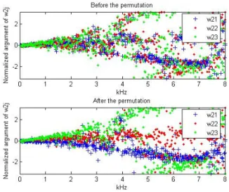
The average SDR achieved by the full-rank unconstrained model, the rank-1 convolutive model as well as binary masking and"0-norm minimization is depicted in Fig. 6. As expected,
all algorithms result in lower separation performance when the source directions are closer due in particular to poorer estimation of the spatial parameters, i.e. spatial covariance matrices Rj(f ) for the full-rank unconstrained model and
mixing vectors hj(f ) for other algorithms. But the full-rank
unconstrained model still outperforms other algorithms in all cases. For instance, when the sources are very close to each other whereα = 50, the full-rank unconstrained model offers
0.9 dB SDR while binary masking only provides 0.2 dB SDR and both rank-1 convolutive model and"0-norm minimization
results in negative SDR. This supports the benefit of the full-rank unconstrained model regardless of the source directions.
E. Blind source separation with the SiSEC 2008 test data
We conducted a fourth experiment to compare the proposed full-rank unconstrained model-based algorithm with state-of-the-art BSS algorithms submitted for evaluation to SiSEC 2008 over real-world mixtures of 3 or 4 speech sources. Two mix-tures were recorded for each given number of sources, using
Fig. 4. Average blind source separation performance over stereo mixtures of three sources as a function of the reverberation time, measured in terms of (a) SDR, (b) SIR, (c) SAR and (d) ISR.
Fig. 6. Average blind source separation performance over stereo mixtures of three sources as a function of the DOA difference between sources.
either male or female speech signals. The room reverberation time was either 130 ms or 250 ms and the microphone spacing 5 cm [5]. The average SDR achieved by each algorithm is listed in Table III for comparison since it provides the overall distortion of the system. The SDR results of all algorithms besides the proposed full-rank unconstrained model-based algorithm were taken from the website of SiSEC 20082, except
for Izumi’s algorithm [15] whose results were provided by its author. T60 Algorithms 3 source mixtures 4 source mixtures 130 ms full-rank unconstrained 3.3 2.8 M. Cobos [21] 2.3 2.1 M. Mandel [22] 0.1 -3.7 R. Weiss [23] 2.9 2.3 S. Araki [24] 2.9 -Z. El Chami [25] 2.3 2.1 250 ms full-rank unconstrained 3.8 2.0 M. Cobos [21] 2.2 1.0 M. Mandel [22] 0.8 1.0 R. Weiss [23] 2.3 1.5 S. Araki [24] 3.7 -Y. Izumi [15] - 1.6 Z. El Chami [25] 3.1 1.4 TABLE III
AVERAGESDROVER THE REAL-WORLD TEST DATA OFSISEC 2008WITH
5CM MICROPHONE SPACING.
For three-source mixtures, the proposed algorithm provides 0.4 dB and 0.1 dB SDR improvement compared to the best current results given by Araki’s algorithm [24] with T60= 130 ms and T60= 250 ms, respectively. For four-source
mixtures, it provides even higher SDR improvements of 0.5 dB and 0.4 dB respectively compared to the best current results given by Weiss’s [23] and Izumi’s algorithms [15]. More detailed comparison (not shown in the Table) indicates that the proposed algorithm also outperforms most others in terms of SIR, SAR and ISR. For instance, it achieves higher SIR than
2
http://sisec2008.wiki.irisa.fr/tiki-index.php?page=Under-determined+speech+and+music+mixtures
all other algorithms on average except Weiss’s. Compared to Weiss’s, it achieves the same average SIR but a higher SAR.
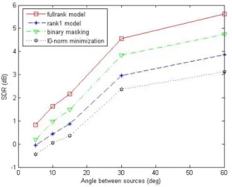
F. Investigation of the robustness to small source movements
Our last experiment aims to examine the robustness of the rank-1 convolutive model and the full-rank unconstrained model to small source movements. We made several record-ings of three speech sources s1, s2, s3 in a meeting room
with 250 ms reverberation time using omnidirectional micro-phones spaced by 5 cm. The distance from the sources to the microphones was 50 cm. For each recording, the spatial images of all sources were separately recorded and then added together to obtain a test mixture. After the first recording, we kept the same positions for s1 and s2 and successively
moved s3 by 5 and 10◦ both wise and counter
clock-wise resulting in 4 new positions of s3. We then applied the
same procedure tos2while the positions ofs1ands3remained
identical to those in the first recording. Overall, we collected nine mixtures: one from the first recording, four mixtures with 5◦
movement of either s2 or s3, and four mixtures
with 10◦
movement of either s2 or s3. We performed source
separation in a semi-blind setting: the source spatial covariance matrices were estimated from the spatial images of all sources recorded in the first recording while the source variances were estimated from the nine mixtures using the same algorithm as in Section IV-B. The average SDR and SIR obtained for the first mixture and for the mixtures with 5◦
and 10◦
source movement are depicted in Fig. 7 and Fig. 8, respectively. This procedure simulates errors encountered by on-line source separation algorithms in moving source environments, where the source separation parameters learnt at a given time are not applicable anymore at a later time.
The separation performance of the rank-1 convolutive model degrades more than that of the full-rank unconstrained model both with 5◦
and 10◦
source rotation. For instance, the SDR drops by 0.6 dB for the full-rank unconstrained model based algorithm when a source moves by 5◦
while the corresponding drop for the rank-1 convolutive model equals 1 dB. This result can be explained when considering the fact that the full-rank model accounts for the spatial spread of each source as well as its spatial direction. Therefore, small source movements remaining in the range of the spatial spread do not affect much separation performance. This result indicates that, besides its numerous advantages presented in the previous experiments, this model could also offer a promising approach to the separation of moving sources due to its greater robustness to parameter estimation errors.
V. CONCLUSION AND DISCUSSION
In this article, we presented a general probabilistic frame-work for convolutive source separation based on the notion of spatial covariance matrix. We proposed four specific models, including rank-1 models based on the narrowband approxima-tion and full-rank models that overcome this approximaapproxima-tion, and derived an efficient algorithm to estimate their parameters from the mixture. Experimental results indicate that the pro-posed full-rank unconstrained spatial covariance model better
Fig. 7. SDR results in the small source movement scenarios.
Fig. 8. SIR results in the small source movement scenarios.
accounts for reverberation and therefore improves separation performance compared to rank-1 models and state-of-the-art algorithms in realistic reverberant environments.
Let us now mention several further research directions. Short-term work will be dedicated to the application of the full-rank unconstrained model to the modeling and separation of diffuse and semi-diffuse sources or background noise. Contrary to the rank-1 model in [12] which involves an explicit spatially uncorrelated noise component, this model implicitly represents noise as any other source and can account for multiple noise sources as well as spatially correlated noises with various spatial spreads. We also aim to complete the probabilistic framework by defining a prior distribution for the model parameters across all frequency bins so as to improve the robustness of parameter estimation with small amounts of data and to address the permutation problem in a probabilistically relevant fashion. Finally, a promising way to improve source separation performance is to combine the spatial covariance models investigated in this article with models of the source spectra such as Gaussian mixture models
[18] or nonnegative matrix factorization [12].
ACKNOWLEDGMENTS
The authors would like to thank Y. Izumi for providing the results of his algorithm on some test data.
REFERENCES
[1] N. Q. K. Duong, E. Vincent, and R. Gribonval, “Under-determined convolutive blind source separation using spatial covariance models,” in
Proc. IEEE International Conference on Acoustics, Speech and Signal Processing (ICASSP), March 2010.
[2] O. Yılmaz and S. T. Rickard, “Blind separation of speech mixtures via time-frequency masking,” IEEE Trans. on Signal Processing, vol. 52, no. 7, pp. 1830–1847, July 2004.
[3] S. Winter, W. Kellermann, H. Sawada, and S. Makino, “MAP-based underdetermined blind source separation of convolutive mixtures by hierarchical clustering and !1-norm minimization,” EURASIP Journal
on Advances in Signal Processing, vol. 2007, 2007, article ID 24717. [4] P. Bofill, “Underdetermined blind separation of delayed sound sources in
the frequency domain,” Neurocomputing, vol. 55, no. 3-4, pp. 627–641, 2003.
[5] E. Vincent, S. Araki, and P. Bofill, “The 2008 signal separation evalua-tion campaign: A community-based approach to large-scale evaluaevalua-tion,” in Proc. Int. Conf. on Independent Component Analysis and Signal
Separation (ICA), 2009, pp. 734–741.
[6] E. Vincent, M. G. Jafari, S. A. Abdallah, M. D. Plumbley, and M. E. Davies, “Probabilistic modeling paradigms for audio source separation,” in Machine Audition: Principles, Algorithms and Systems, W. Wang, Ed. IGI Global, to appear.
[7] N. Q. K. Duong, E. Vincent, and R. Gribonval, “Spatial covariance models for under-determined reverberant audio source separation,” in
Proc. 2009 IEEE Workshop on Applications of Signal Processing to Audio and Acoustics (WASPAA), 2009, pp. 129–132.
[8] C. F´evotte and J.-F. Cardoso, “Maximum likelihood approach for blind audio source separation using time-frequency Gaussian models,” in Proc.
2005 IEEE Workshop on Applications of Signal Processing to Audio and Acoustics (WASPAA), 2005, pp. 78–81.
[9] E. Vincent, S. Arberet, and R. Gribonval, “Underdetermined instanta-neous audio source separation via local Gaussian modeling,” in Proc.
Int. Conf. on Independent Component Analysis and Signal Separation (ICA), 2009, pp. 775–782.
[10] A. P. Dempster, N. M. Laird, and B. D. Rubin, “Maximum likelihood from incomplete data via the EM algorithm,” Journal of the Royal
Statistical Society. Series B, vol. 39, pp. 1–38, 1977.
[11] H. Sawada, S. Araki, R. Mukai, and S. Makino, “Grouping separated frequency components by estimating propagation model parameters in frequency-domain blind source separation,” IEEE Trans. on Audio,
Speech, and Language Processing, vol. 15, no. 5, pp. 1592–1604, July 2007.
[12] A. Ozerov and C. F´evotte, “Multichannel nonnegative matrix factoriza-tion in convolutive mixtures for audio source separafactoriza-tion,” IEEE Trans.
on Audio, Speech and Language Processing, vol. 18, no. 3, pp. 550–563, 2010.
[13] T. Gustafsson, B. D. Rao, and M. Trivedi, “Source localization in re-verberant environments: Modeling and statistical analysis,” IEEE Trans.
on Speech and Audio Processing, vol. 11, pp. 791–803, Nov 2003. [14] H. Kuttruff, Room Acoustics, 4th ed. New York: Spon Press, 2000. [15] Y. Izumi, N. Ono, and S. Sagayama, “Sparseness-based 2CH BSS using
the EM algorithm in reverberant environment,” in Proc. 2007 IEEE
Workshop on Applications of Signal Processing to Audio and Acoustics (WASPAA), 2007, pp. 147–150.
[16] B. D. van Veen and K. M. Buckley, “Beamforming: a versatile approach to spatial filtering,” IEEE ASSP Magazine, vol. 5, no. 2, pp. 4–24, 1988. [17] J.-F. Cardoso, H. Snoussi, J. Delabrouille, and G. Patanchon, “Blind separation of noisy Gaussian stationary sources. Application to cosmic microwave background imaging,” in Proc. European Signal Processing
Conference (EUSIPCO), vol. 1, 2002, pp. 561–564.
[18] S. Arberet, A. Ozerov, R. Gribonval, and F. Bimbot, “Blind spectral-GMM estimation for underdetermined instantaneous audio source sep-aration,” in Proc. Int. Conf. on Independent Component Analysis and
Signal Separation (ICA), 2009, pp. 751–758.
[19] G. McLachlan and T. Krishnan, The EM algorithm and extensions. New York, NY: Wiley, 1997.
[20] E. Vincent, H. Sawada, P. Bofill, S. Makino, and J. Rosca, “First stereo audio source separation evaluation campaign: data, algorithms and results,” in Proc. Int. Conf. on Independent Component Analysis
and Signal Separation (ICA), 2007, pp. 552–559.
[21] M. Cobos and J. L´opez, “Blind separation of underdetermined speech mixtures based on DOA segmentation,” IEEE Trans. on Audio, Speech,
and Language Processing, submitted.
[22] M. Mandel and D. Ellis, “EM localization and separation using interau-ral level and phase cues,” in Proc. 2007 IEEE Workshop on Applications
of Signal Processing to Audio and Acoustics (WASPAA), 2007, pp. 275– 278.
[23] R. Weiss and D. Ellis, “Speech separation using speaker-adapted eigen-voice speech models,” Computer Speech and Language, vol. 24, no. 1, pp. 16–20, Jan 2010.
[24] S. Araki, T. Nakatani, H. Sawada, and S. Makino, “Stereo source separation and source counting with MAP estimation with Dirichlet prior considering spatial aliasing problem,” in Proc. Int. Conf. on Independent
Component Analysis and Signal Separation (ICA), 2009, pp. 742–750. [25] Z. El Chami, D. T. Pham, C. Servi`ere, and A. Guerin, “A new model
based underdetermined source separation,” in Proc. Int. Workshop on