Coupled near and far field thermal plume analysis using finite element techniques

COUPLED NEAR AND FAR FIELD THERMAL PLUME ANALYSIS USING FINITE ELEMENT TECHNIQUES

by

John T. Kaufman and E. Eric Adams

Energy Laboratory Report No. MIT-EL 81-036 October 1981

COUPLED NEAR AND FAR FIELD THERMAL PLUME ANALYSIS USING FINITE ELEMENT TECHNIQUES

by

JOHN TAYLOR KAUFMAN

and E. ERIC ADAMS Energy Laboratory and R.M. Parsons Laboratory for

Water Resources and Hydrodynamics Department of Civil Engineering Massachusetts Institute of Technology

Cambridge, Massachusetts 02139

Sponsored by

Northeast Utilities Service Company and

New England Power Company under

M.I.T. Energy Laboratory Electric Utility Program Energy Laboratory Report No. MIT-EL 81-036

ABSTRACT

The use of the open cycle cooling process for thermal power plants requires significant effluent discharges into aquatic environments. Both engineering and environmental considerations require accurate prediction of resulting temperature distribution in the receiving waters. Most predictive models have looked at one of two distinct regions of the discharge--the near or the far field--to the neglect of the other.

A methodology is developed in this work to combine the attributes of both near and far field models. A finite element far field code is utilized which calculates both the circulation and heat distribution over a large area of the domain. From the far field coarse grid, a semi-circular area is removed which corresponds to the near field region of the discharge. At the new edge of the domain, which represents the near-far field boundary, mass flux and temperature boundary conditions are specified which simulate both the discharge into and entrainment out of the domain resulting from the surface discharge jet.

Initial verification and testing of the model's characteristics is carried out in a hypothetical idealized domain. A more realistic

veri-fication is done at two prototype sites by comparing calculated results to previously acquired field data. The two sites are Millstone Nuclear Power Station (on Long Island Sound near Waterford, Connecticut) operating with two units and Brayton Point Generating Station (in Mt. Hope Bay near

Somerset, Massachusetts) operating with three units on open cycle (existing conditions) and with four units on open cycle (proposed future condition). These comparisons suggest that the model can realistically describe the far

field flow patterns associated with near field mixing thus making the model a useful tool in evaluating induced circulations, the source of entrained organisms, etc. These flow patterns are a direct function of the near field entrainment and discharge distributions which are specified as model boundary conditions and are thus easily calibrated and, if

necessary, modified. Comparison between measured and predicted temperatures indicates that the predicted lengths and areas of isotherms are similar to measured lengths and areas. Predicted temperatures generally indicate greater dispersion than measured temperatures thus leading to overprediction of intake recirculation. Also, because boundary conditions on the near-far boundary have been assumed constant, the shape of predicted isotherms is not as responsive to changes in ambient current direction (e.g., tidal varia-tions) as the measurements indicate.

Future efforts should emphasize grid and program coding refinement to improve computational efficiency, use of methods to reduce numerical dispersion and incorporation of time-varying near-far field boundary conditions.

ACKNOWLEDGMENTS

The work described in this report was performed in connection with the project "Near and Far Field Interaction of Thermal Discharges" through the MIT Energy Laboratory Electric Utility Program. The authors wish to thank Northeast Utilities Service Company and New England Power Company for their generous support and utility steering committee members Mr. Ron Klattenberg, Dr. William Renfro, Dr. Jerry Holm and Mr. Andrew Aitken for their cooperation.

The research was performed by Mr. John Kaufman, a Research

Assistant in the Department of Civil Engineering under the supervision of Dr. E. Eric Adams of the Department of Civil Engineering and the MIT Energy Laboratory. Substantial assistance was also provided by Mr. Peter

Ostrowski, a Research Assistant in the Department of Civil Engineering and Dr. Keith Stolzenbach, Associate Professor of Civil Engineering.

Finally, thanks are due to Mrs. Carole Soloman for her assistance in preparing the report.

TABLE OF CONTENTS Page No. TITLE PAGE ABSTRACT ACKNOWLEDGMENTS TABLE OF CONTENTS LIST OF FIGURES LIST OF TABLES CHAPTER I INTRODUCTION CHAPTER II BACKGROUND 2.1 Nature of Problem

2.2 Near Field vs. Far Field Problem 2.3 Review of Models

CHAPTER III THEORETICAL DESCRIPTION 3.1 General Approach 3.2 Far Field Model 3.3 Near Field Model

3.4 General Use of the Model CHAPTER IV IMPLEMENTATION

4.1 Idealized Domain 4.2 Millstone Plant Site 4.3 Brayton Pt. Site CHAPTER V SUMMARY AND CONCLUSIONS

5.1 Summary 5.2 Conclusions

5.3 Suggestions for Further Research REFERENCES 11 13 13 16 18 28 28 29 35 41 48 48 61 79 117 117 117 119 121

No. Figure 2-1: Figure 2-2: Figure 2-3: Fiugre 2-4: Figure 2-5: Figure 3-1: Figure Figure Figure 3-2: 4-1: 4-2: Figure 4-3: Figure 4-4: Figure Figure 4-5: 4-6: LIST OF FIGURES Title Characteristics of a Discharge from a Surface Channel

Characteristics of a Submerged Multiport Diffuser

Coupling of Near and Far Fields (after Adams et al., 1975)

Schematic of Parameterized Temperature Prediction Model (after Stolzenbach, 1971) Schematic of Cooling Pond Model Formulated by Watanabe et al., 1975

Description of Surface Jet Parameters Used in Model Schematization

Near Field Surface Jet Properties

Discharge and Entrainment Flow Relationship Results from CAFE Run at Practice Domain with Constant Cross-Current and No Intake Results from CAFE Run at Practice Domain with No Cross-Current and an Intake DISPER Calculation with Practice Domain

Corresponding to CAFE Run Shown in Figure 4-3 Site of Millstone Nuclear Power Station

Grid Used for Millstone Simulations

Page No. 14 15 23 25 27 45 46 54 56 57 60 62 67

No. Figure 4-7: Figure 4-8: Figure 4-9: Figure 4-10: Figure 4-11: Figure 4-12: Figure Figure 4-13: 4-14: Figure 4-15: Figure 4-16: Figure 4-17: Title

CAFE Run Results at Millstone Under Stagnant Conditions

CAFE Run Results at Millstone Under Maximum Flood Tidal Conditions

CAFE Run Results at Millstone Under Maximum Ebb Tidal Conditions

DISPER Results at Millstone Under Stagnant Conditions

DISPER Results at Millstone Under Flood Tidal Conditions

DISPER Results at Millstone Under Ebb Tidal Conditions

Site of Brayton Point Generating Station Large, Coarse Grid Used at Brayton Point Simulation

Transitional Grid Portion Between Near-Field-Far-Field Interface and Coarse Grid

Large View of Mt. Hope Bay CAFE Results Under Maximum Flood Conditions for Three Unit

Operation

View of Region Near Discharge at Brayton Pt. Showing CAFE Results Under Maximum Flooding Conditions For Three Unit Operation

Page No. 70 71 72 73 74 75 80 83 84 90 91

No. Figure 4-18: Figure 4-19: Figure 4-20: Figure 4-21: Figure 4-22: Figure 4-23: Figure 4-24: Figure 4-25: Title

View of Region Near Discharge at Brayton Pt. Showing CAFE Results Under High Slack

Conditions for Three Unit Operation Large View of Mt. Hope Bay CAFE Results Under Maximum Ebb Conditions for Three Unit Operation

View of Region Near Discharge at Brayton Pt. Showing CAFE Results Under Maximum Ebb

Conditions for Three Unit Operation

View of Region Near Discharge at Brayton Pt. Showing CAFE Results Under Low Slack

Conditions for Three Unit Operation Large View of Mt. Hope Bay CAFE Results Under Maximum Flood Conditions for Four Unit Operation

View of Region Near Discharge at Brayton Pt. Showing CAFE Results Under Maximum Flood Conditions for Four Unit Operation

View of Region Near Discharge at Brayton Pt. Showing CAFE Results Under High Slack

Conditions for Four Unit Operation Large View of Mt. Hope Bay CAFE Results Under Maximum Ebb Conditions for Four Unit Operation Page No. 92 93 94 95 96 97 98 99

No. Figure 4-26: Figure 4-27: Figure 4-28: Figure 4-29: Figure 4-30: Figure 4-31: Figure 4-32: Figure 4-33: Figure 4-34: Figure 4-35: Title

View of Region Near Discharge at Brayton Pt. Showing CAFE Results Under Maximum Ebb

Conditions for Four Unit Operation

View of Region Near Discharge at Brayton Pt. Showing CAFE Results Under Low Slack

Conditions for Four Unit Operation

DISPER Results at Bryaton Pt. for Three Unit Operation Under Maximum Flood Conditions DISPER Results at Brayton Pt. for Three Unit Operation Under High Slack Conditions

DISPER Results at Brayton Pt. for Three Unit Operation Under Maximum Ebb Conditions

DISPER Results at Brayton Pt. for Three Unit Operation Under Low Slack Conditions

DISPER Results at Brayton Pt. for Four Unit Operation Under Maximum Flood Conditions DISPER Results at Brayton Pt. for Four Unit Operation Under High Slack Conditions

DISPER Results at Brayton Pt. for Four Unit Operation Under Maximum Ebb Conditions DISPER Results at Brayton Pt. for Four Unit Operation Under Low Slack Conditions

Page No. 100 101 103 104 105 106 110 111 112 113

No. Table Table Table 2-1:

3-1:

4-1:

Integrated Analysis Solutions and Parameter Definition

Summary of Near Field Surface Jet Properties Near Field Parameters Computed

for Idealized Domain Simulation Near Field Parameters Computed

for Millstone Simulation (Two Units) Comparison of Measured Isotherm Lengths

(range, ft) and Predicted Isotherm Length (value in parentheses, ft) for Various Tidal Phases at Millstone Station

Near Field Parameters Computed for Brayton Pt. Simulation Page No. 26 42 51 65 78 86

CHAPTER I INTRODUCTION

For power plants employing once through cooling, it is necessary to accurately predict induced temperatures and flow fields in the re-ceiving water body. Such prediction may be necessary for two general reasons: first, accurate prediction of induced temperatures and veloci-ites is a first step in assessing potential environmental impacts.

Possible impacts include entrainment at the intake of small organisms into the condenser cooling system, impingement of larger organisms onto intake screens and exposure of organisms to elevated temperatures within the discharge plume. Federal and state agencies often place specific limitations on induced temperatures and/or induced velocities out of respect for such possible impacts.

The second consideration involves design limitations on intake temperature. Power plant efficiency decreases with increasing intake temperature. In considering the design (or redesign) of intake and dis-charge structures, a utility must account for possible increases of temperatures at the intake, due to recirculation of the thermal plume, which might lead to a lower plant efficiency or may even require derating. Accurate thermal prediction models may, therefore, aid significantly in optimizing cooling system design.

The wide range of time and space scales characterizing the thermal structure of the water body increases the difficulty in plume modeling. A characteristic of many thermal discharge flow fields is the presence of two distinct regions of flow: the near field and the far field.

Most modeling efforts concentrate on one of these regions to the neglect of the other. This is because of major problems in dealing with the two very different scales of the two regions. The difficulty in coupling the two regions leads to very approximate means of modeling the actual physics of the problem.

This thesis describes a method which combines existing knowledge of near field induced temperature and flow disturbances with available far field numerical models. The resulting tool can be used to address these near and far field interactions. In applying this

techni-que, emphasis will be placed on evaluating the model's ability to simu-late near-far field interaction with respect to both environmental con-siderations and engineering design constraints.

CHAPTER II BACKGROUND

2.1 Nature of Problem

Steam-electric power plants using once-through condenser cooling systems are often located near large water bodies. Shorelines of coastal areas, large lakes and river banks serve this purpose and are utilized widely. This study concentrates on coastal sites due to the interests of the sponsors. The general approach could easily be ex-tended to a river application, though.

The heated effluent from a power plant is typically discharged into the aquatic environment either through a surface discharge channel or a

submerged diffuser. Drawings of the two configurations are shown in Figures 2-1 and 2-2. In the surface discharge case heated water with flow rate Q and density p enters through a discharge channel with a certain geometry into receiving waters with variable depth H, ambient density p and ambient current velocity distribution u . A submerged

a a

diffuser may be characterized by similar discharge variables except that the method of discharge would be through a number of discharge ports near the bottom of the receiving body rather than through a shore-line channel. A detailed discussion of these two discharge types may be found in Adams et al., 1979. The work done in this research has focused on surface discharges; however, the approach could be extended easily to submerged diffusers.

SIDE

VIEW

PLAN VIEW

Pa

Shore

SIDE VIEW PLAN VIEW /

I

Characteristics of a Submerged Multiport Diffuser. Figure 2-2:

2.2 Near Field vs. Far Field Problem

A number of techniques have been developed for predicting the excess temperature distribution induced in the receiving water by the heated discharge from power plants. Yet, new methods are desired to accurately deal with the diverse influences acting on these temperature distributions. Both natural and man-made processes affect these distri-butions. Any temperature prediction technique must address this problem of combined ambient and man-made thermal influences. Yet it is hard to model all of these processes at a single time in a single analysis, due to the widely varying spatial scales of the near and far fields.

The near field is defined as that region whose characteristics are dominated by the initial discharge conditions. These include the discharge velocity and corresponding momentum,and the discharge

tempera-ture rise and corresponding buoyancy. In the near field, the temperatempera-ture reduction within the plume results primarily from induced mixing of the discharge with the receiving water. Large velocity gradients exist

relative to those found at greater distances from the point of discharge. The length of the near field is typically of the order of 1000 ft. and the temperature rise is in the range 1-100 F above ambient after mixing.

The near field circulation induced by the cooling water discharge depends on the type of outfall structure. The discharge may be taken to be one or more mass and momentum jet(s) discharging to the ambient

region. These jets can alter the natural flow field by inducing flow from the far field for entrainment along the sides of the jet. Also,

the jet itself has a large influence on the flow field. After dilution, the jet flow is typically of order 10,000 cfs which is significant!

The far field is defined as that region of the plume which is largely independent of the initial characteristics of the discharge. This region is dominated by the natural processes of water movement, dispersion, and surface heat loss. Tidal flushing and its associated dispersive effects dominate the far field temperature distribution at the type of coastal plant sites studied in this work. Surface heat loss is the ultimate sink (from the water's point of view) over the large areas represented by the far field. In rough absolute terms,

the far field extends out from the area effected by the discharge jet to the end of the domain being modeled. A range of distance may be estimated as 0.5 to 10 miles.

At intermediate distances from the point of discharge the plume is still being affected by the initial buoyancy and momentum, but it is also being influenced by natural water movement and dispersive processes. Because of the distinctive properties of this transition region it is often referred to as the intermediate field. The scale of the inter-mediate field ranges from about 1000 ft to the order of 1 mile,

depend-ing on the discharge characteristics. The large size of this region is a major reason why a link between near and far field modeling is

necessary.

Instead of combining near and far field effects, models usually concentrate primarily on either the near or the far field. Near field models (eitlher physical, integral jet or numerical) typically assume

that the far field characteristics (receiving water temperature, velocity, etc.) are known with the consequence that the effect of the near field on the far field can't be computed. Far field models, on the other hand, tend to over simplify near field effects by considering simply an influx of mass and heat (or in some instances only an influx of heat) at the point of discharge. Near field mixing, if accounted

for at all, must be treated by the assignment of artificial values of dispersion coefficient. This procedure discounts many influences of

the near field on the far field. Because of the difficulty in near-far field coupling, certain aspects of interest, such as mixing zones, correct entrainment, flow fields and shoreline impacts are difficult to assess.

2.3 Review of Models

Near Field Surface Jet

Most near field surface jet analyses can be divided into three types: _{integral jet models, numerical models or physical (hydraulic} scale) models. Examples of integral jet analyses include: Stolzenbach and Harleman, 1971; Shirazi and Davis, 1974; and Prych, 1972. In the

integral approach, the 3-D equations are integrated over the jet cros-section resulting in a numerically one-dimensional formulation. That is, numerical integration is only required in the longitudinal coordin-ate. Jet properties such as trajectory, width, depth, centerline

velocity, centerline temperature, and flow rate are thus determined as a function of longitudinal coordinate. This procedure has usually

described well the near field characteristics of the jet, particularly at sites with simple geometry, deep water and relatively high discharge Froude number. One problem inherent with these models, however, is the failure to consider re-entrainment influences on the jet and near field region from the far field. In general, these integral jet models require explicit specification of boundary conditions which represent the in-fluence of the far field on the near field model. This is a limitation as transient effects within the far field's heat distribution aren't accounted for within the specified boundary conditions. It is not

poss-ible to know the real thermal boundary conditions for this problem due to the effects of surface heat exchange, convective mixing, land bound-aries and other far field temperature influences. Another problem with these models is that their range of applicability is limited to a com-paratively short distance from the discharge point where the near field processes indeed govern the flow. (A more detailed discussion on this distance may be found in Section 3.) Often, however, temperature esti-mates are required in the intermediate field, requiring that the near field results be extrapolated--perhaps unrealistically.

Other approaches to the near field have been developed using both physical and numerical modeling techniques. Physical modeling presents a similar problem due to the boundaries on the model. Sides (and ends) of containing tanks where the models are built are often too close to

the discharging jet to simulate the open receiving waters of most coastal areas. Numerical models of the near field suffer similar pit-falls in the speccflication of far field influenced boundary conditions.

Far Field Models

Several models have been developed which concentrate on the trans-port of constituent concentration or heat through the far field (Ahn and Smith, 1972; Leimkuhler, 1974; Wang and Connor, 1975; Eraslan, 1974; Siman-Tov, 1974). _{These models generally share many of the same} char-acteristics. For instance, due to the generally large and complicated nature of the far field, most models are numerical. Many have the char-acteristic of dealing only with a 2-D formulation to simplify the calcu-lations. Because of the longer time scales of interest for the far field, most models are transient.

Numerical models of the far field have utilized both finite differ-ence and finite element solution techniques. For example, to compute

horizontal circulation (i.e. surface elevation n and horizontal velocities u and v), a finite difference method would approximate the governing

differential equationsof continuity and of x and y momentum conservation by corresponding difference equations associated with discrete grid points. The result is a set of simultaneous linear algebraic equations which is

solved by matrix techniques. The finite element approach uses the

Galerkin method of weighted residuals. In this method a continuous solution for T, u and v would be assumed by interpolating between trial values of n, u and v defined at nodal points. The method seeks those trial values for which the weighted residual (error) between the trial and real solution is minimized when integrated over the element.

Characteristic of the two methods is the shape of the elements used in the schematization of the domain. The finite difference method

typically utilizes square elements of constant size with the nodal points at the four corners or the center. This is a constraint on

modeling the domain as it is often not possible to adequately match land boundaries using square shaped elements of fixed size. Finite elements are more flexible in both size and shape. Their absolute size is restricted only by the consideration of describing the physical

gradi-ents in the system. In other words, the elements must be small enough to allow sufficient discretization of areas where large gradients in velocities or depth exist. The shape of the elements should approximate

equilateral triangles, though this is not a strict requirement. The degrees of freedom in the elements' size and shape allow the irregular boundaries of domains to be modeled quite closely. It also makes

poss-ible the transition from smaller elements in areas of large gradients to larger elements in the less varying far field. More comparisons between finite difference and finite element techniques may be found in Pinder and Gray, 1977.

In general, it is difficult to model accurately the numerous

processes taking place in a far field region. Specific problems concern the specification of boundary conditions, especially at open boundaries, and near the point of discharge. Inability in the latter regard means that it is difficult to represent the near field influence in these far field models. To illustrate, if a jet discharging into a receiving water body has an initial flow rate of Qo and a dilution ratio of 10,

the total amount of flow entering the far field region will be 10Qo, and the amount of flow leaving the far field (associated with jet

en-trainment) would be 9Qo . Most standard far field models would typically

specify only the net input of lQo

-Integrated or Complete Field Models

Models which attempt to combine near and far field characteristics seem to hold the most promise in predicting heat distributions about thermal discharges. Koh and Fan, 1970, presented a coupled integral near field model with a two dimensional (longitudinal and vertical) numerical model of the far field. This type of coupling allows the near

field effects to be represented as boundary conditions in the far field, but does not allow far field effects to be represented in the near field. For example, it cannot handle reversing currents where far field heat is returned to the near field.

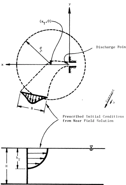
Adams et al., 1975, modeled far field temperature distributions using the concept of relative diffusion. The far field model transported

heat in the form of discrete patches which were advected, dispersed and decayed in accordance with physical far field processes. The initial size and temperature of these patches was derived from near field

analysis. A major advantage of this type of model is that it can model the influence of transient ambient currents which can advect heat back

into the near field (see Figure 2-3).

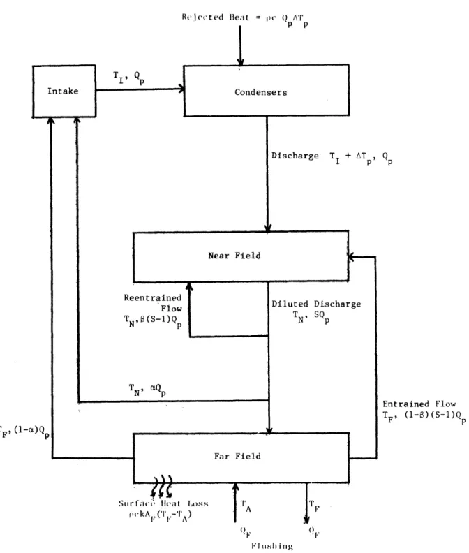
In the work of Stolzenbach, 1971, an integrated approach was presented which incorporated the major interaction between power plant and receiving water in essentially a three box model including power

Discharge Point

/

I

I

I

Prescribed Initial Conditions from Near Field Solution

H

H

U__

Figure 2-3: Coupling of Near and Far Fields (after Adams et al., 1975). (xT ,

plant intake, near field mixing region and far field zone. See Figure 2-4. Linkage between these boxes was described by the plant operating variables (e.g., flow rate and temperature rise) and by

several parameters describing the feedback between regions (e.g., an intake recirculation coefficient, near field dilution and re-entrain-ment coefficient,and far field flushing and heat loss parameters). While quite simple, such a model can represent all of the relevant

interaction in complex receiving waters such as enclosed tidal embay-ments. The solution for intake, near field and far field temperature rises, along with parameter definition are provided in Table 2-1.

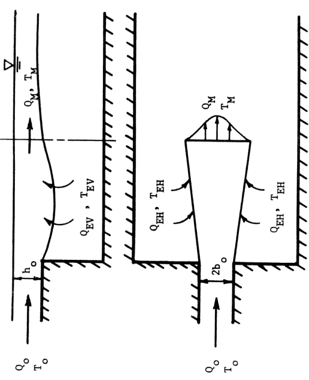
Watanabe et al., 1975, developed a two layer cooling pond model which describes both major regions, the near and far fields (see Fig-ure 2-5). The entrance mixing zone was modeled by the Stolzenbach-Harleman surface jet model. The far field surface layer was analyzed using a finite element method formulated in terms of temperature, stream function and vorticity. The lower layer was represented by the Ryan-Harleman mathematical model for a stratified reservoir. The primary interest of this model to the present study is the manner in which Watanabe specified the discharge flow from the jet into the com-putational domain. He accounted for entrained flux into the sides of the jet through specified flows, QEH and QEV. This additional mass was then added to the discharge into the domain at a rate QM. These boundary concepts were utilized directly in the present model's formu-lation.

Rejected Heat = pe Q AT a P p Discharge T_I + AT _pp, Q Entrained Flow TF, (1-8)(S-1)Q F() i (ls

Figure 2-4: Schematic of Parameterized Temperature Prediction Model (after Stolzenbach, 1971).

Table 2-1: Integrated Analysis Solutions and Parameter Definition QpATp T _F = TA + A _{QF + kAF} AT TN = TF +S(l-8) + 8 -a AT I F +S(1-8) + 8 -a

TA = Ambient temperature of the far field region TF = Averaged far field temperature

AF = Effective surface cooling area of far field QF = Far field flushing flow

Qp = Condenser water flow

AT = Condenser temperature rise TN = Near field temperature

T = Intake temperature

S = Near field dilution, i.e. - ratio of mixed flow leaving near field to discharge flow (S=1 implies no mixing)

8 = Fraction of the entrained flow originating in the near field at temperature TN (8=0 implies no re-entrainment)

a = Fraction of intake water drawn from the near field. The remainder is supplied by the far field (a=0 implies no recirculation)

rXI Ce

CY

O O 0 0

CY E- _{CY H}

Figure 2-5: Schematic of Cooling Pond Model Formulated by Watanabe et al., 1975.

CHAPTER 3

THEORETICAL DESCRIPTION

3.1 General Approach

The formulation of this model begins with a far field schematiza-tion of the main porschematiza-tion of the domain under study. Into this domain (which may represent a bay, lake or coastal area), a jet discharge enters near the power plant site. In this model, a semi-circular area is carved out around the discharge jet plume and physically removed from the schematized domain. The portion left represents the inter-mediate and far fields of the region. It is assumed that the near

field area which was removed can be modeled by specifying (inside) boundary conditions on the far field which match those influences by,

the discharge jet. In these examples, the near field characteristics were determined using analytical and empirical results from other

surface jet studies. More detailed discussion of these determinations will be covered in this chapter.

The model used for this work makes use of two distinct, yet inter-connected numerical models designed to calculate flow and mass concen-tration distributions, respectively. The finite element circulation model CAFE was developed by Wang and Connor, 1975. The mass dispersion

finite element model DISPER was written by Leimkuhler, 1974, with an original emphasis on sediment transport processes. The two programs were written in conjunction which made their coupled use easier.

3.2 Far Field Model

The CAFE and DISPER Models

CAFE is formulated for vertically integrated variables in the far field. Circulation patterns and surface elevation changes are cal-culated at individual nodal points to simulate continuous movement throughout the domain. This technique eliminates dependence on the vertical coordinate. This is justified when little variation in the variables takes place over depth.

Most concern over temperature rises in power plant receiving waters takes place in the summer months when temperature levels are at their highest. This period coincides with the greatest stratification due to surface warming, both from the ambient meteorology and the artificial thermal loading, from the plant. This justified use of the 2-D mixed layer approach of CAFE since the density structure would resemble

two distinct layers. Because of the density difference between the two layers upon stratification, mixing between them is reduced.

One of the output sets from CAFE contains nodal fluxes and water depths which are used by DISPER to represent the circulation in the domain being modeled for concentration distribution. To this field ambient artificial heat inputs were added. Previous applications of DISPER involved concentration of sediment from a proposed sediment dis-posal (Pearce and Christodoulou, 1975), the concentration of larval fish near a power plant (Chau, 1977), and various other applications dealing with pollutant dispersion in coastal areas (Pagenkopf et al., 1976).

concentra-tions over the same prescribed depth as used in CAFE. In traditional uses of such models, the user has the option of running the models

with the whole depth, fully mixed (as may be necessary in the wintertime when the whole depth is fully mixed), or with a smaller stratified top layer which is fully mixed in its depth. This is an important point as a basic limitation of a 2-D model is its inability to accurately repre-sent the third dimension. This study's model was concerned with induced stratification on the upper surface layer. The far field plume depth was determined from near field jet properties (Eq. 3.3-7) and this value was input as the constant depth throughout the far field. Ostrowski, 1980, in a related effort used full depths in both of the same numerical models. His work was more concerned with natural temper-ature distributions as contrasted with the description of the thermal plume in the intermediate field in this study. For another comparison, NUSCO, 1975, modeled circulation near Millstone using the full depth and dispersion using partial depth.

The forms of the governing equations used by CAFE are given as follows. For a complete derivation of these and related expressions, see Wang and Connor, 1975.

n+ + = q₁ (3.2-1) at ax ay I + +q fq -g(h+n) a1L +T

at

ax

(q+ q

aF

aF

S

n

Q f-h udz 4 -h

qy fh vdz

-h

q = a mass input to the system

u,v = the flow velocities in the x,y directions f = coriolis parameter, 2wearth sin

Searth = angular frequency of the earth's rotation = latitude (N) of the location

g = gravitational acceleration

h = the depth of the water body at mean low water

s 2

T = CD AIRU30

PAIR = air density [m 0.075 pcf]

U_{3 0} = wind speed 30 ft above sea surface -3 C = (1.1 + 0.0536 U 30)0.10 p = density of water 2 Cf = g /3 (Manning's n) q F = E x xx xx ax

aqx aq F =E ( +x.) xy xy ay ax

3q

Eij = the eddy viscosity coefficient

As in the solution of all differential equations, it is necessary to specify both initial and boundary conditions. In all cases these specifications are chosen to model as closely as possible the real physical domain. For points in the interior of the domain, initial

conditions may be specified as,

(qqy) y (xo(x,y),qyo(x,y)) for all (x,y) in the interior domain at t = 0 H = h + r = H (x,y) for all (x,y) at t - 0

0

The discharge boundary conditions are summarized for the normal and tangential directions as,

qn _{anxqx + anyy} qn

qs nyx nx y s

where,

a = cos(n,x); a = cos(n,y)

and the superscript * signifies a prescribed value. A detailed des-cription of the method in which these nodal boundary conditions are applied in the context of an idealized site may be found in Sec. 4.1.

DISPER solves the vertically integrated form of the conservation of energy equation. The final governing expression is,

30 +3u 3v_ 3 a s 3t x 3y 3x Qx y y pc V where, 0 = Tdz = TH (3.2-5) -h

T = the water temperature at various depths Q _x = -E -- -E --xx

8x

Q

c = heat flux source [Joules/m3 sec]

c = specific heat of water at constant volume

The model may be formulated in terms of either actual or excess temperature above ambient (T in 3.2-5). The appropriate choice depends on whether the model is used to predict natural temperatures as well as artificially induced temperature variation. Ostrowski, 1980, was con-cerned with natural warming and computed actual temperatures while this

study focuses primarily on excess temperatures. Because the time scales of processes which affect excess temperaturcs are shorter (order of one day rather than order of a week for natural temperature prediction),

this requires less computation time. The disadvantage is that one has to estimate the background temperature if one wants to estimate actual temperatures from excess temperatures.

Program Modification

A number of modifications have been made to CAFE and DISPER in order to make them more flexible and able to perform computations directly with heat (temperature), rather than mass (concentration).

Ostrowski, 1980, modified CAFE to allow time-varying fluxes (inflows and outflows of water) to be used as boundary conditions. Both constant and

sinusoidal fluxes can be specified at the edges of the domain. This makes it possible to model tidal flows into and out of the domain without depend-ing on the raisdepend-ing and lowerdepend-ing of ocean boundaries to simulate tidal forcdepend-ing. By specifying the fluxes, more direct control exists over the flow in

the domain. Such a modification was also necessary to handle the fluxes at the near field-far field (inner) boundary. An accounting of the verification of this is in Stolzenbach et al., 1980.

DISPER was revised by Ostrowski to solve directly for temperature in the basic convective-diffusion equation rather than constituent concentrations. As stated previously, calculations can either be made for excess temperature or for the actual temperature. Excess

tempera-ture calculations are made using the source/sink terms , assuming first order dependence between heat loss and excess temperature. Thus,

*s

where,

o

K = the equilibrium heat transfer coefficient

K is treated as a constant so this approach doesn't take into account the temporal variation of meteorology.

For actual temperature calculations, Ostrowski, 1980, added a

subroutine which computes surface heat transfer at each element using net heat flux equations with time-varying meteorology. The model takes the meteorological inputs from which it calculates the heat loss or gain s This simulation is superior to the constant sink or source option in allowing temporal variability of heat loss calculations. The details

of these heat calculations may be found in Ostrowski, 1980.

Murakami developed a scheme to optimally number nodal points in the finite element grid (Stolzenbach et al., 1980). This numbering scheme was necessary to minimize the band width of the matrix used in the numer-ical routine which solves the matrix equations. The basis for this program was found in references on finite element applications to structural analysis.

3.3 Near Field Model

A separate group of governing equations may be derived for the surface jet models which most near field analyses relevant to this work have used. These expressions have been left out of this work, but can be found in other references (e.g., Stolzenbach and Harleman, 1971).

From these governing equations an important scaling parameter, the local lulenisi metric roiide number, is derived:

B = , -1/2 (3.3-1)

L

_P

a where,

u,Ap and k represent characteristic values of jet velocity, density deficiency and length at varying positions along the jet.

In a buoyant jet, the value of IFL decreases along the axis. Near the point of discharge of the jet into the receiving waters IFL is typically in the range of 5 to 15. In developing the near field characteristics which were used to determine boundary conditions on the intermediate field portion of the domain, several physical parameters were derived as a function of the densimetric Froude number at the origin.

It should be noted that the discharge densimetric Froude number may be calculated using two different jet length scales. It is normally defined (symbol IF ) in terms of the depth, ho of the discharge channel. However, it may also be defined (symbol IF') using the square root of

o

one-half of the channel crossectional area, o, as characteristic length. Thus

IF'= u = IF (ho/b )1 /4 (3.3-2)

o

o

where,

b = the half-width of the discharge channel

o

= (h b )1/2 (3.3-3)

o oo

The significance of IF' is that it utilizes a more representative char-o

acteristic jet length scale and has been found to provide better corre-lation of results of different length to width ratios.

The near field properties used in this model, are based on Jirka et al., 1981. That paper describes surface jet properties using the Stolzenbach and Harleman surface jet model, along with laboratory and field data. These properties are defined in Figure 3-2 and discussed briefly below.

As mixing takes place the jet spreading rate db/dx increases and the local Froude number IFL decreases. The distance at which IFL becomes

of order 1 is referred to as the transition distance because it is at this point that buoyant spreading begins to dominate jet mixing and thus the underlying assumptions of the near field no longer hold. This con-dition is usually signaled in integral jet models by a concon-dition of rapid jet spreading and/or by a singularity in the matrix of differential equa-tions. For the Stolzenbach-Harleman model, this transition occurs at

IFL = 1.6. The distance, xt, at which this occurs correlates with,

x = 12 IF' (h /b )-0.2 (3.3-4)

t o0 o o

h

or, for moderate values of the aspect ratio (.1 <

-b-

- b - t

o given by,

x - 15R F' . (3.3-5)

t oo

The maximum depth h to which a plume would spread in deep re-max

ceiving waters provides an indication of the ultimate plume thickness in the intermediate field. This depth is predicted from the Stolzenbach-Harleman model as

h = 0.42k F' (3.3-6)

max oo

Measurements in the laboratory and the field (e.g., Stolzenbach and Harleman, 1971; and Stolzenbach and Adams, 1979, respectively) suggest that the plume thickness in the intermediate field is approximately one half of the maximum jet thickness or

h - 0.21 IF' (3.3-7)

Of course other processes acting in the intermediate and far fields will affect the plume thickness, so Eq.3.3-7 is just an approximation. The distance to the plume region of maximum penetration is given as,

x = 5.5£1F' (3.3-8)

max oo

Equation 3.3-8 will be used later to analyze the effects of shallow

receiving water on jet dilution.

As the discharge jet enters the receiving waters the total amount of flow in the jet body increases as water is entrained from the sides. This dilution is significant in reducing temperatures in the near field and in creating flow which must enter the far field. For our purposes, jet mixing is characterized by the total, or stable, volumetric dilu-tion Ss defined as the ratio of the jet flow Q to the discharge flow Qo i.e.,

Ss =

Q/Qo

This dilution is referred to as stable because it is the asymptotic value of dilution which is reached beyond the transition distance at which point buoyancy effects have succeeded in damping further turbulent

entrainment. For the Stolzenbach-Harleman model under conditions of deep receiving water andIF' _{O -}> 3,

S = 1.41' (3.3-10)

s o

The volumetric dilution Ss is inversely related to the average tempera-ture rise at the end of the near field, AT . Thus,

AT

o = S = 1.4' (3.3 - 11)

Peak (centerline) temperatures at the end of the near field AT are cs higher than the average temperature by a factor which depends on the lateral profiles of temperature and velocity in the jet. With the Stolzenbach-Harleman model, the predicted stable centerline temperature rise is given by AT - S = 1.01F' (3.3-12) AT cs o cs

where S is the corresponding centerline dilution. cs

The total jet entrainment, E , can be expressed as,

E = S -1 _(3.3-13)

S S

This entrainment may be broken up into the components of total entrain-ment in the vertical and horizontal directions. These factors, E and Eh,are given for IF' > 1 as,

0 Es = Ev + Eh (3.3-14) E = 1.2 (IF'-l) _(3.3-15) v 0 Eh = 0.2 (F' + 1) (3.3-16) h o

These relationships indicate how flow conditions with large F' lead to o

large vertical entrainment relative to the horizontal entrainment. As IFo 00 E /Eh - 6. This implies small far-field lateral recirculation for moderate or large W' and vice versa. However, it is noted that in shallow water, vertical entrainment may be wholly or partly inhibited, thus decreasing overall dilution and enhancing the effect of lateral recirculation.

Shallow waters have a significant effect on jet behavior and mixing characteristics, particularly in light of the large bottom

entrainment contribution indicated for deep water jets (Eq. 3.3-14-16). For shallow conditions, bottom entrainment flow must approach laterally through a restricted fluid layer under the jet. Induced velocities become higher leading to more frictional dissipation, pressure

devia-tions below hydrostatic and a reduced vertical entrainment flow. Very shallow receiving waters with bottom attachment lead to reduced mixing capacity and distorted jet cross-sectional geometry.

To account for the effects of shallowness on the dilution ratios, a new parameter is defined--h /H--where h is the computed maximum

max max

depth of an equivalent deep water jet (3.3-6) and H is the depth of water at the point of maximum jet penetration x (3.3-8). Generally,

max

for small values of h /H laboratory and field measurements indicate max

good agreement with deep water model results; for larger values of h /H, induced temperatures are increased and the ultimate mixing is

max

decreased. The ratio of observed to calculated values of centerline dilution, S cs gives an indication of the degree of shallowness,

S cs

r S (3.3-17)

cs where,

r = shallow water dilution reduction factor

s

A

S = observed centerline dilution in shallow water cs

S = predicted centerline dilution for deep water cs

As the value h max/H increases, this dilution factor decreases. From max

data accumulated on the effects of dilution, it appears that for ratios of h < 0.75 the deep water dilution prediction S (Eqn. 3.3-12) is

max cs

a reliable value. Therefore, a criterion which is used to determine shallow water conditions is,

h

max > 0.75

(3.3-18) H

Further field and laboratory work compiled by Jirka et al., 1981, has shown that a reasonable factor for adjusting dilution values to account for shallowness is,

0.75 0.75

rs (h H) for h x /H > 0.75. (3.3-19) max

3.4 General Use of the Model

The various surface jet properties described in the previous sec-tion are summarized in Table 3-1. Figure 3-1 shows how this informasec-tion is used in the model schematization. The reader is also referred to the description of the idealized domain covered in Section 4.1.

The transition distance, defined by Eqn. 3.3-5, was used as a guide-line in establishing the inside boundary of the computational domain between the near and far fields. This boundary consisted of a layer of

small elements which surrounded the near field. The elements were small here to give greater resolution of velocity and temperature, since it is at this point that the largest gradients exist.

Moving out from the near-far boundary, the elements increase in size. This corresponds to the lower gradients as the distance from the

TABLE 3-1 Summary of Near Field Surface Jet Properties SCALING PARAMETERS: u IF' = o o Apo 1/2 (- go)/ o o

DENSIMETRIC FROUDE NO,

DISCHARGE CHANNEL CHARACTERISTIC LENGTH

DEEP WATER PROPERTIES:

h

h

X

SHALLOW WATER DILUTION

x = 15 2, IF' t o o = 0.42 X IF' max o o = 0.21 X IF'

far

o

o

MAXIMUM PLUME DEPTH

FAR FIELD PLUME DEPTH

DISTANCE FROM DISCHARGE TO MAX PLUME DEPTH

STABLE VOLUMETRIC DILUTION = Q/Qo = AT

/AT

STABLE CENTERLINE DILUTION = AT /AT

o cs

VERTICAL JET MASS ENTRAINMENT

HORIZONTAL JET MASS ENTRAINMENT

S 0.75 0.75 rs h /H(x ) max max h max (for H(x ) > 0.75) max

SHALLOW WATER DILUTION

jet source increases. Numerically, the model has a limit on the differ-ence in size of two adjacent elements. Nodes are then spaced to reduce the gradient in element size. As the distance from the near field in-creases, the larger size of the far field elements becomes roughly

constant. A majority of the domain has elements of similar size because of this. The average length of a far field element side is about 15-20 times that of an average element adjacent to the near field.

Another consideration in developing the finite element grid is the optimum element shape for maximizing numerical stability. It has been found from previous finite element models that equilaterally shaped triangular elements serve best. In developing the grids for this

study's domains, elements of equal side lengths were used as extensively as possible. However, in some cases departures from the equilateral shape were necessary. This was caused by both the increasing element size from near to far and the real physical constraints of land bound-aries. Actual shapes of the elements were kept as close as possible to equilateral, but sometimes the constraints yielded significantly non-uniform elements. A general "limit" which was adopted for element uniformity was that no internal angles should be greater than 900.

Boundary conditions for the two numerical models used, CAFE and DISPER, are satisfied by designating the type of node and the type of boundary (element side) for each element on the boundary of the domain. Any land or ocean boundary condition, with or without fluxes may be accounted for with this system. In CAFE, a land boundary is one in which boundary fluxes are specified. These boundaries are identified to the program by naming the contiguous nodal points forming each

boundary. All other boundaries in the CAFE model are designated ocean boundaries. On these boundaries, the (tidal) elevation n is specified

but there is no explicit constraint on fluxes.

CAFE allows the classification of boundary nodes in several differ-ent categories depending on whether the boundary is land or ocean.

Land boundary nodes require that normal flux be specified. This flux is specified at each node but represents, both physically and to CAFE, the flux which passes through the land boundary corresponding to each land boundary node. Thus this flux is specified as flow per unit width

(e.g., ft2/sec). This boundary condition was used to represent the dis-charge from the near field, the entrainment flow to the near field, the plant intake flow, river inflow, and the vertical entrainment flow leaving the domain (see Figure 3-1). In certain cases, flux across a land boundary was also used to represent ambient currents. At all other land boundaries, a condition of no normal flux was specified.

For each land boundary node, the option was available to specify no flux tangential to the boundary at a boundary node (no slip condition). This was necessary in situations where sharp corners existed on the

boundary. By specifying the no tangential flux boundary condition, the flow was routed away from these areas preventing accidental loss of mass (and heat in the DISPER calculation) across these boundaries. In CAFE, purely land boundary nodes are designated as either type 1 (allowing tangential flux) or type 4 (no tangential flux allowed).

Ocean boundary nodes in CAFE have their tidal amplitude specified. Using a sinusoidally varying function to describe the ambient raising

EvQ o a) Top View Q 0 _TO EQ vo

--

I

alf

width

Full width

K

I:!

Is~

Transition

epth

Near Field Surface Jet Properties.

y

FO-20

15

10

I

A

_/

_Fo

A'/

F

oFo'

F

0

₀

and lowering of the tide, flow was forced into the domain through the boundary sides. There also was available a provision in the model to

input phase lags in the tidal elevation for each of the boundary nodes. The expression used in the model which governs the tidal forcing is,

2x

S= a[l-cos(T- (t-))] _(3.4-1)

where,

= the height of the water level above the mean low water mark a = the amplitude of the tidal fluctuation

T = the tidal period of the region under study = the phase lag

The phase lag can be used to account for spatial and temporal variations of the flow coming into the domain. For instance, a long open ocean boundary may have a tidal flow which comes into one portion of the bound-ary prior to coming into the other parts.

It is also possible to combine the node type specifications of normal/tangential fluxes and tidal heights. The tidal heights and normal flux specifications may or may not include the constraint on the tangential flux. The specification of normal flows and tidal heights correspond to points where land and ocean boundaries meet.

Since DISPER utilizes the flow field produced by CAFE, the specifi-cation of a no flux boundary has no meaning as far as mass flux is con-cerned. This type of boundary does constrain the heat from crossing the boundary, however. This distinction is important to consider in avoiding problems with artificial heat buildup. Individual boundary node types aren't specified in the running of DISPER.

CHAPTER IV IMPLEMENTATION

To test the working characteristics and validity of the model, it was necessary to apply it to field sites with the necessary descriptive data with which to compare the results. Isotherms measured at various

phases of a tidal cycle at the Millstone and Brayton Pt. sites were used to check against the results of the numerical computations. Prior to this step, though, the basic nature of the model was tested using an idealized domain. This was done to simulate the use of the coupled

near-far parameterization and to check sensitivities to certain numerical factors.

4.1 Idealized Domain Purpose

Up to the beginning of this project the computer models, CAFE and DISPER, were used only for far field analysis. The modification of

these models to include near field influences represented a large change in their use which called for certain interim checks. Various program modifications were tested and are reported in a project progress report

(Stolzenbach et al., 1980). Application of the program was tested using an idealized practice domain discussed here. By making use of the

relatively simple and symmetrical geometry the results of various tests could be examined more quickly than at an actual site.

Grid Design

The domain which was used can be seen in Figs. 4-2 and 4-3. It was rectangular shaped (2740 ft. x 5480 ft.) with a constant depth of

13 ft. This constant depth included the side boundaries, both water and land. _{In designing the practice domain it was desired to use a simple,} symmetrical scheme to provide, as much as possible, a control in which the formulation and numerical properties of the model could be tested. This justified the use of the constant depth specification.

The near field region was carved from the base of the rectangular domain. From this symmetric, semi-circular boundary the triangular finite elements radiated out to a limiting maximum size. The transition was gradual to avoid large differences in member lengths. The minimum element side length on the grid was 82 ft. This is contrasted with the maximum element side length of 1250 ft. The radius of the semi-circular

near field area was roughly 360 ft.

To simulate the influence of the near field on the far field model, flux boundary conditions were specified on the near field-far field

interface for CAFE. These boundary fluxes were selected to be representa-tive of typical near field mixing from a surface discharge. See Table 4-1 and Figs. 4-2 and 3. Over the central three nodes of the transition circle, the discharge was represented by flux values of 27.3 ft2/sec. Both sets of side entrainment nodes had flux values of 8.4 ft2/sec

specified at each nodal point. Sensitivity to alternate lateral entrain-ment relationships is discussed later in this chapter. To account for

tlle vertIca l entcrnan[nment from Lhe domain into the jet plume,mass was removed from tihe domain along tlie top boundary of the grid at a rate of 0.75 ft /sec. _{Also, in certain runs, an intake was established by} re-moving flux from the lower right-hand corner of the domain. The flux

specified was 3.3 ft2/sec over a distance of 1400 ft. Several runs were made using specified influx on the left end of the domain and an equal and opposite outflux along the right boundary of the domain. This was to simulate a steady cross current into which the plume was discharged. The value specified was a uniform current velocity of 0.66 ft/sec. _{The full set of near field boundary conditions on the} far field may be seen in Table 4-1.

Boundary Node Specification

In specifying boundary conditions for the practice domain, it was desired to use a realistic, yet relatively simple configuration. For the CAFE run, both domain side boundary types and boundary node types were specified. A land boundary was specified around the entire prac-tice domain. All nodes were type 1 (specified normal) except the six corner ones which were type 4 (specified normal and no tangential). The two ends of the rectangular domain had specified fluxes to simulate a steady, constant cross current. This could have been modeled as well by tidal amplitude specifications on the boundary.

The boundaries in DISPER were specified such that only the lengths where no mass flux was removed were left as a land boundary. The open

boundaries included the near-far field boundary, the two open ends, and the top boundarywhere vertical entrainment flow was removed.

Time Step

The time step used while running CAFE was found to be dependent on four physical characteristics of the problem: (i) Maximum flow

Table 4-1: Near Field Parameters Computed for Idealized Domain Simulation

Parameter*

Discharge Flow Rate

Discharge Temperature Rise Transition radius

Near Field Volumetric Dilution

Vertical Mass Entrainment Horizontal Mass Entrainment

Far Field Plume Depth Shallow Water Dilution

Correction Symbol Q (m3/sec) O AT (OC) rt(m) S Simulation Value 62.9 13.5 118.9 4.5 E V Eh hfar (m) r s 1.0 2.5 4.0 1.0 *see Table 3-1

velocity, u; (ii) Minimum nodal spacing, a; (iii) Eddy viscosity, Eij; and (iv) Wave speed, c = gJ. The practice domain's minimum spacing was 82 ft., the maximum velocity was 2.7 ft/sec, and the wave speed was 20.5 ft/sec, and for most runs, the eddy viscosity was 165 ft2/sec. The most successful timestep was 2.0 secs. Values

significantly greater than this caused numerical instability character-ized by uncontrolled spatial oscilllations in the water elevation at certain nodes, ultimately resulting in negative values of n which ex-ceeded, in absolute value, the actual water depth H. Values of At less than 2.0 secs produced similar circulation patterns as observed with 2.0 sec but with increased computation time.

The following general criteria were available to determine the necessary timestep for running DISPER (Leimkuhler et al., 1975):

R2 10 At < -- _D (4.1-1) 10 At < (4.1-2) where, At = time step D = dispersion coeff.

Applying the physical characteristics to 4.1-1 and 4.1-2, a range of At from 2 to 10 secs. was determined corresponding to a range in the value of D from 110 to 22 ft2/sec.

In addition to the above criterion on the time step, a condition for stability involving just the three physical quantities has been observed (Leimkuhler et al., 1975):

Ru

-< 2 (4.1-3)

For a given k and u, this expression gave guidelines on the appropriate range of D (D > _{100) while Eqns. 4.1-1 and 4.1-2 then dictated time step.} It should be noted that Eqn. 4.1-3 in particular is not a precise cons-traint. Use of values of D lower than suggested resulted in spatial oscillations of predicted temperatures. However, even for values of D significantly greater than suggested (215-275 ft2/sec), these oscilla-tions weren't completely eliminated. It is also worth noting that the value of dispersion coefficient required for numerical purposes, given by Eq. 4.1-3, is about an order of magnitude greater than that which would exist physically due to real sub-grid scale dispersion effects. See further discussion under simulation results. The choice of D thus involves a tradeoff between numerical accuracy (suggesting a large value) and physical accuracy (suggesting a small value). Results presented later in this section were run with a D value of 110 ft2/sec and a time step of At = 13 sec. The fact that these integration

parameters didn't fall within the limits of the numerical stability criteria point out the approximate nature of this criteria.

Entrainment Distributions

Several distributions _{of discharge and entrainment boundary} condi-tions at tlhe near-far f ield Interface were investigated in the practice domain. One featured a gradual decrease of entrainment from the

semi-circular base to the transition from entrainment to discharge

a) Gradual Variation between Entrainment and Discharge.

b) Constant Discharge and Entrainment Flow Boundary with Sharp Transition.

c) Discharge and Entrainment Flow Distribution Used in Simulations. Figure 4-1: Discharge and Entrainment Flow Relationship.

node with smaller discharge values on the two adjacent nodes. Another distribution (Figure 4-2b) had a constant influx value across the two entrainment sides with an abrupt shift to a constant outward flux at the three discharge nodes. Both of these flux distributions led to numerical instability, however. A final configuration was chosen which had cons-tant entrainment values along the two sides and over the discharge nodes. The two nodes between the entrainment and discharge were left with no

specified normal flow, though. This avoided a sharp discontinuity in flux values of adjacent nodes which enhanced stability. This form is shown in Figure 4-ic.

Simulation Results

Initially, the simplest types of CAFE simulations (stagnant water, no intake) were made to investigate senstivity to time step and the different configurations of the flux boundary conditions on the near-far boundary. Eventually the optimum flux set was determined to be that depicted in Figure 4-1c.

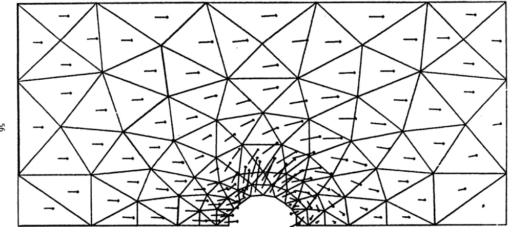
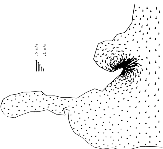
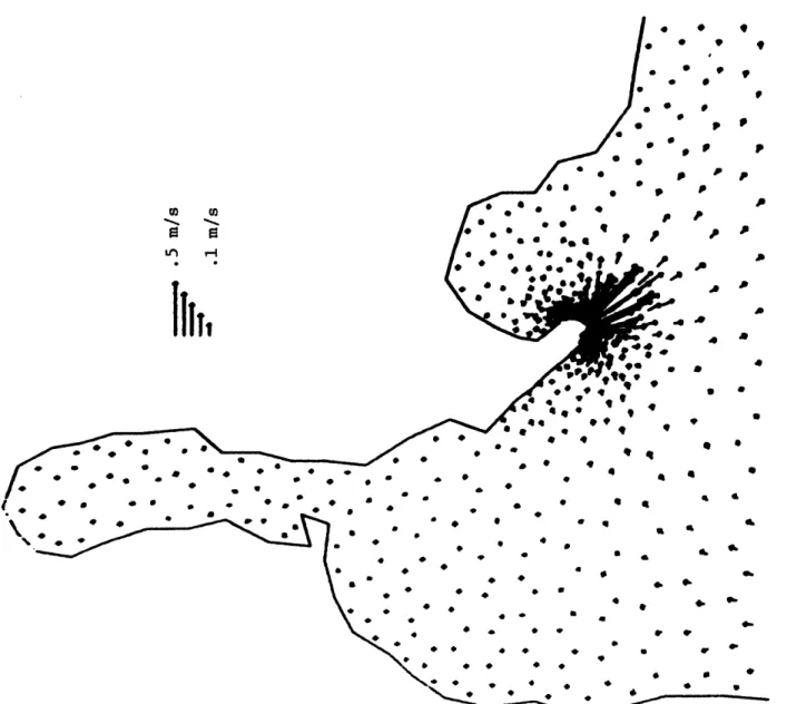
Subsequent to this CAFE runs were made with an intake and with a 0.2 m/s cross-current. Steady state circulation patterns corresponding to a 0.2 m/s cross-current with no intake and stagnant conditions with an intake are shown in Figures 4-2 and 4-3.

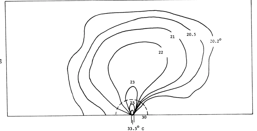
After experimenting with CAFE, the heat dispersion model DISPER was implemented. This involved specifying excess temperature boundary conditions of 3.00 C at the discharge nodes and using the circulation patterns created by CAFE. The excess temperature of 30 C corresponds to a power plant discharge temperature of 13.50 C and a dilution of

00

Figure 4-2: Results from CAFE Run at Practice Domain with Constant Cross-Current and No Intake.

Plant Intake Figure 4-3: _{Results from CAFE Run at Practice Domain with No Cross-Current and an Intake.}