A coupled kinetic Monte Carlo–finite element
mesoscale model for thermoelastic martensitic
phase transformations in shape memory alloys
The MIT Faculty has made this article openly available.
Please share
how this access benefits you. Your story matters.
Citation
Chen, Ying, and Christopher A. Schuh. “A Coupled Kinetic
Monte Carlo–finite Element Mesoscale Model for Thermoelastic
Martensitic Phase Transformations in Shape Memory Alloys.” Acta
Materialia 83 (January 2015): 431-447.
As Published
http://dx.doi.org/10.1016/j.actamat.2014.10.011
Publisher
Elsevier B.V.
Version
Author's final manuscript
Citable link
http://hdl.handle.net/1721.1/106611
Terms of Use
Creative Commons Attribution-NonCommercial-NoDerivs License
Detailed Terms
http://creativecommons.org/licenses/by-nc-nd/4.0/
1
Coupled kinetic Monte Carlo-finite element mesoscale model for thermoelastic martensitic phase transformations in shape memory alloys
Ying Chen1*, Christopher A. Schuh2
1 Department of Materials Science and Engineering, Rensselaer Polytechnic Institute, 110 8th Street,
Troy, NY 12180, USA
2 Department of Materials Science and Engineering, Massachusetts Institute of Technology, 77
Massachusetts Avenue, Cambridge, MA 02139, USA
A mesoscale modeling framework integrating thermodynamics, kinetic Monte Carlo (KMC), and finite element mechanics (FEM) is developed to simulate displacive thermoelastic transformations between austenite and martensite in Shape Memory Alloys (SMAs). The model is based on a transition state approximation for the energy landscape of the two phases under loading or cooling, which leads to the activation energy and rate for transformation domains incorporating local stress states. The evolved stress state after each domain transformation event is calculated by FEM, and is subsequently used in the stochastic KMC algorithm to determine the next domain to transform. The model captures transformation stochasticity, and predicts internal phase and stress distributions and evolution during the entire incubation, nucleation, and growth process. It also relates the critical transformation stresses or temperatures to internal activation energies. It therefore enables quantitative exploration of transformation dynamics and transformation-microstructure interactions. The model is used to simulate superelasticity (mechanically-induced transformation) under both load control and strain control in single crystal SMAs under uniaxial tension.
Keywords:
Martensitic phase transformation Kinetic Monte Carlo
Finite elements Shape memory alloys Superelasticity
2
1. Introduction
Thermoelastic Shape Memory Alloys (SMAs) have broad applications in sensing, actuation, energy conversion, and damping [1]. They can switch between their original shape and a notably different shape under thermal or mechanical cycling, and this process usually involves a temperature or stress hysteresis indicative of energy dissipation [2-4]. The shape memory and superelastic properties of SMAs are achieved by a reversible and diffusionless martensitic phase transformation that occurs mainly by a large, cooperative shear of atoms [5]. The transformation process (i.e., the nucleation and growth of thermoelastic martensite plates) involves extensive interactions with defects, including interfaces and surfaces. For example, martensite plates may preferentially nucleate at these defects [6, 7], and may also interact with them at the transformation front [8]. The crystallographic shear by which martensite develops can lead to mechanical interactions across both phase and grain boundaries [9], as well as strain relief at free surfaces.
Transformation-microstructure interactions, however, are not well understood, and their effects on transformation kinematics have not been established quantitatively. The need to gain a fundamental understanding of the roles of defects is further motivated by recent results showing size effects in small-scale SMAs. For example, grain size effects on transformation temperatures and stresses emerge below a critical size of about 100 μmin polycrystalline SMAs [10-13]. In single crystalline SMA pillars with diameters below 20 μm, pillar size clearly affects the transformation stresses [14-17]. In SMA microwires [18] and foams [19-21] with bamboo grain structures (i.e., with grain sizes equal to the wire diameter or strut thickness), the characteristics of transformation also depend on the sample size. These size effects have been attributed to the increasing relative density of grain boundaries or free surfaces at smaller scales, but their origins and microstructural mechanisms have just begun to be explored. Modeling martensitic transformation processes at the microstructural level can shed light onto the interplay between transformation processes and grain boundary or surface states, and perhaps eventually to microstructure design of SMAs.
The majority of existing models for SMAs are analytical and generally fall into the following categories. (1) Phenomenological theories of martensite crystallography, which examine the conversion pathways
between two crystal structures in terms of distortion (or shearing) and rotation [22-25].
(2) Dislocation-based models of martensite interfaces, which use dislocation arrays to model interface structure and mobility based on the known properties such as stress fields of dislocations [26-31]. (3) Thermodynamic models of martensitic nucleation [32-34] and transformation [35-38], which focus on
the contribution to the free energy change from interface energy, elastic energy, and dissipation mechanisms.
(4) Constitutive micromechanical models for martensitic transformation, which determine macroscopic behaviors based on an assumed local stress-strain constitutive law and advance transformation by
3
gradually changing a state variable such as martensite fraction [39-44].
These models provide profound understanding of martensitic transformation, mechanistically, thermodynamically and mechanically. But they in general neither involve a physical time scale nor address spatial phase distributions and evolution. Few of these models have been used to explore the effects of defects on transformation kinematics, and many are not suited to this purpose.
Computational models for reversible martensitic transformations in SMAs are relatively rare. There are relatively few atomistic studies such as molecular dynamics (MD) of SMAs [45, 46] and most deal with the binary NiTi system [47, 48], since they rely on the availability of accurate inter-atomic potentials for complex SMAs. The limited length (e.g., 10-30 nanometers) and time (e.g., nanoseconds) scales accessed by such MD studies are not directly comparable to those (e.g., hundreds of nanometers [49] to micrometers in size and milliseconds [17] to minutes in time) involved in existing experimental measurements of SMAs. There are also some finite element [50-55] and phase field [56-60] models for SMAs, which can incorporate much larger scales in the constitutive laws describing material energy during transformation. However, continuum models sometimes cannot predict reverse transformation, and more generally tend to lack connections between simulated scales and those intrinsic to martensitic transformation in SMAs, which are essential for understanding defect-transformation interactions.
All of the above points speak to the need for a physically-based mesoscale model for thermoelastic martensitic transformation, one that can include a physical timescale for transformation, and specifically address issues of transformation kinematics in the presence of microstructure. Our purpose in this paper is to develop such a mesoscale modeling framework for SMAs by coupling the kinetic Monte Carlo (KMC) algorithm with the finite element method (FEM). FEM allows us to determine the mechanical state everywhere in the material, and to allow the local state to affect the transformation sequence. The onset and progression of the transformations are controlled by KMC using a transition-state rate equation characteristic of thermally-activated phenomena, and the forward and reverse transformations are treated “symmetrically” in the model, i.e., they are both permitted at any time. In what follows we develop the framework for such a mesoscale model, and demonstrate its capabilities to simulate mechanically-induced transformations under conditions of constant loading rate and constant strain rate.
2. Thermodynamic Framework for Thermoelastic Reversible Martensitic Transformations
In this section, we examine the energetics governing austenite↔martensite transformations in SMAs. In Section 2.1, we determine the free energies of the two phases as functions of temperature and stress, as the difference between them is the driving force for transformation. In Section 2.2, we formulate the system energy evolution during transformations, which involves a variety of additional sources such as interface energy, strain energy, and dissipated energy. In Section 2.3, we propose an apparent equilibrium
4
temperature/stress, and determine the transformation hysteresis incorporating coupled temperature-stress effects. In Section 2.4, we use an energy landscape approach to describe the above thermodynamic driving forces and energy penalties for transformations. Lastly, in Section 2.5, we present a new type of energy landscape map describing conversions between an initial state and a transformed state, which will lay the foundation for our subsequent kinetic Monte Carlo-Finite Element mesoscale modeling in Section 3. In the following, we use “A” and “M” to denote properties of austenite and martensite, respectively.
2.1. Free Energy Difference between Austenite and Martensite
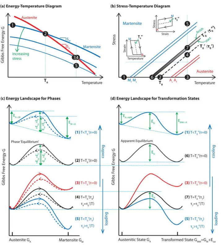
The Gibbs free energies and per unit volume as a function of temperature T are illustrated in Fig. 1(a). When there is no external stress, (red line) and (bold blue line), where and
are the chemical free energies. The slopes of these lines are the entropy SA and SM, respectively.
and (1)
Let T0 denote the equilibrium temperature at which , , and the transformation enthalpy ∆
, , , , ∆ , where ∆ 0 and ∆ 0. As , and
, , where is the density and is the specific heat capacity, the transformation enthalpy at T is
∆ ∆ ∆ (2)
with ∆ . Meanwhile, , / and , / , and therefore the
transformation entropy at T is
∆ ∆ ∆ / (3)
where and ∆ 0, and as a result decreases with T more slowly than as can be seen in Fig. 1(a). Eqs. (2) and (3) lead to the change in chemical free energy at T, ∆ ∆ ∆ .
∆ ∆ ∆ / (4)
If the change in heat capacity is assumed insignificant and ∆ 0, Eq. (4) is reduced to
∆ ∆ (5)
When , ∆ 0, and austenite is preferred; when , ∆ 0, and martensite is preferred. Upon application of an external stress that leads to a resolved shear stress on the habit plane (in the elastic regime before yielding), GA changes little while GM is strongly biased because the elastic strain is
insignificant compared to the transformation simple shear strain . We estimate and . Therefore, decreases with increasing stress, shown by the thinner blue lines in Fig. 1(a).
∆ ∆ (6)
A third term, , where P is the pressure, may be introduced into Eq. (6) for transformations involving a significant volumetric strain , which is not considered in this paper. Introducing Eq. (5) into Eq. (6), we obtain
5
∆ ∆ (7)
where is a stress-dependent equilibrium temperature below which martensite is preferred.
∆ (8)
Accordingly, there is a temperature-dependent equilibrium stress . ∆
(9)
increases with , and increases with T. This behavior is further depicted in the stress-temperature diagram in Fig. 1(b), where the black dashed line corresponds to or . It intercepts the temperature axis at T0, i.e., 0 , and its slope is / ∆ / . For example, using parameters for a Cu-Al-Ni SMA [18], 0.1154, atomic volume 0.013 nm , transformation enthalpy of -330 J/mol, and assuming 300 K, we obtain ∆ 4.2 10 J/m , ∆ 1.4 10 J/ K ∙ m , and / 1.2 MPa/K. This is consistent with a tensile stress-temperature slope of 2-3 MPa/K observed experimentally for the same alloy considering the Schmid factor [9, 61]. In the regime left to (or above) the line, martensite is preferred, but martensitic transformation is not guaranteed because the transformation process involves energy penalties as will be described below.
2.2. System Free Energy Evolution during Transformation
During transformation, the change in the Gibbs free energy density (i.e., per unit volume) of a sample involves many sources. In rate form,
↔ ∆ ∆ (10)
In Eq. (10), σ is the external stress ( 0 for thermal cycling). The rate of martensite volume fraction change 0 and the strain rate 0 during forward transformation, while during reverse transformation 0 and 0. is the austenite/martensite interface energy per unit area, and Ai i is the interfacial area
density. ∆ is the difference in surface energy per unit area, and multiplies the specific surface area Asf; this term pertains to the intersection of the phases with free surfaces, and would only be relevant for some geometries where such intersections are energetically significant. Eel is the average increment in elastic strain energy density.
The changes in chemical free energy, interfacial energy and surface energy, as well as the stored elastic strain energy due to forward transformation are recovered during reverse transformation when changes its sign. The frictional work is irreversible and is positive in both transformation directions [7, 36, 62]. We define the recoverable energy other than chemical energy as Eise, whose subscripts ‘ise’ stand for contributions from interfacial, surface, and elastic strain energies.
∆ (11)
6
∆ ↔ ∆ (12)
where 1 during forward and 1 during reverse transformations. Introducing Eqs. (7) and (8) into Eq. (12), we obtain
∆ ↔ ∆ (13)
and recall that ∆ 0.
Eqs. (12) and (13) can be used to distinguish between the driving forces and energy penalties for transformations; negative quantities drive the transformation while positive ones oppose it. During A→M forward transformation ( and 1), the 1st term is negative and is the driving force, while the 2nd and 3rd terms are positive and are penalties. During M→A reverse transformation ( and 1), both the 1st and 2nd terms are negative and are the driving forces, while the 3rd term is positive and is the penalty. The additional driving forces needed to overcome the energy penalties shift the transformation temperatures away from the equilibrium temperature .
Now consider martensite nucleation. While the driving force per unit volume for phase transformation is usually constant in classical thermodynamic treatments of nucleation, the 1st term in Eq. (13) depends on the local resolved shear stress (see Eq. (7)). not only depends on the applied stress but also on the transformed volume Ω, which affects the interactions between transformed and untransformed volumes. The 2nd and 3rd terms depend on Ω in an even more complicated manner, as the transformation generates and annihilates interfaces, interacts with other defects, etc. Nevertheless, because of their different dependencies on Ω, a critical volume Ω needs to be exceeded in order to bring ∆ → below zero. 2.3. Apparent Equilibrium Temperature/Stress and Transformation Hysteresis
Further examining Eq. (13), the term shifts transformation temperatures but does not affect hysteresis, because its sign reverses with the transformation direction. Hysteresis arises from the additional driving force required to compensate the non-recoverable component in both transformation directions. We rearrange Eq. (13) into only two terms, one dictating the net driving force and the other dictating the hysteresis.
∆ ↔ ∆ (14)
where is the apparent equilibrium temperature. While (or at finite stresses) is a material property, is a sample property. The midpoint method (e.g., adding half of the hysteresis to Ms or taking the
average of Ms and As) commonly used in experiments [61] to estimate the equilibrium temperature yield
rather than .
7
increases with stress due to the 2nd term in Eq. (15), consistent with observations in thermal cycling experiments under a constant external stress (i.e., stress-assisted two-way shape memory effects) [18]. The 3rd term in Eq. (15) renders dependent on sample geometry and size, as well as the transformed phase fraction. Because is generally positive and ∆ 0, at any stress level. Eq. (15) also leads to an apparent equilibrium stress for mechanical cycling at a constant temperature T.
∆
(16) where at any temperature. As illustrated in the insets in Fig. 1(b), and may vary during transformations, depending on how varies with martensite fraction fM (e.g., a constant slope would
indicate a linear relationship with fM).
The dependence of and on fM triggers variations in transformation temperatures or stresses, giving
rise to the slopes on the strain-temperature or stress-strain curves in the transformation portion. An otherwise single transformation temperature (stress) is spread over a range from “start” to “finish” temperatures (stresses); these are sketched as a pair of lines (blue for martensite and red for austenite) in Fig. 1(b). We show (and ) in Fig. 1(b) as a band, whose intercept with the temperature axis is approximately bounded between , /2 and , /2 during cooling. The A→M forward transformation occurs at ΔG → 0 and M→A reverse transformation occurs at ΔG → 0. Therefore, Eq. (14) leads to
→ → /∆
→ → /∆ (17)
Plugging Eq. (15) into Eq. (17) leads to the temperature-stress relationships during transformations.
→ ∆ →
→ →
→ ∆ →
→ → (18)
Eq. (18) directly yields transformation hysteresis. For thermal cycling, the temperature hysteresis is
∆ T → → ∆ → →
→ → → →
→ → → → (19)
For mechanical cycling, the stress hysteresis (expressed in resolved shear stress) is
∆ → → ∆ → → → → → → → → → → (20) Eqs. (19) and (20) explicitly incorporate the coupled temperature-stress effect in hysteresis. For example, the ∆ → → / term in Eq. (20) quantitatively explains the classical rate effect in bulk or large SMA specimens [63], which exhibit larger stress hysteresis due to temperature excursions (as a result of
8
relatively sluggish heat transfer at higher rates). Eqs. (19) and (20) may be reduced to a single term ( 2 /∆ or 2 / ) if → → and → → , which however may be oversimplified in some cases. We next incorporate the above thermodynamic understanding into the energy landscape map.
2.4. Energy Landscape for Phases
While the above analytical transformation thermodynamics is deterministic (i.e., ∆ ↔ 0 is required), the energy landscape description is a probabilistic approach. It depicts the energies of possible configurations, with the stable or metastable ones occupying local minima. A configuration can change to any another, with a probability depending on the energy barrier along the conversion pathway.
Fig. 1(c) shows the energy landscape for transformations between austenite and martensite, with an arbitrary reaction coordinate along the x-axis (which may somehow be viewed as strain since the transformation is displacive). The five curves correspond to the five conditions (① to ⑤ in the stress-temperature space in Fig. 1(b), and the energy of the preferred phase at each condition has also been marked in Fig. 1(a). The vertical positions of these curves reflect their relative energy magnitudes. Curve ③ can be viewed as an initial, high temperature, zero stress condition where and austenite is preferred. ③→②→① shows free energy changes during cooling at zero external stress, and ③→④→⑤ shows free energy changes due to loading at a temperature above Af. At ② and ④ when ,
, and the two phases have an equal probability of existence. At ① and ⑤, , and the preferred phase becomes martensite.
Let us first examine the equilibrium case of ② (or ④) when and . The free energy change during transformation in Eq. (13) or (14) becomes
Δ ↔ (21)
The energy penalty for forward transformation ( 1) is while that for reverse transformation is , which is lower, due to the recovery of (e.g., interfacial and elastic strain energies). We construct the energy landscapes by imposing kinetic barriers with heights equal to their respective energy penalty above the free energy of the phases. In Fig. 1(c), the energy landscapes for forward and reverse transformations are sketched as solid and dashed lines, respectively. The two will collapse into one only if
0, which is the requirement for an ideal phase equilibrium but is rarely the case.
At other temperatures and/or stresses when and , we impose the same energy barriers above the average of and , as demonstrated for curve #1 in Fig. 1(c). Accordingly, the energy barriers for forward and reverse transformations are
9
→ ∆
→ ∆
(22) With decreasing temperature or increasing load, , and → decreases and → increases. → does not have be decreased to zero in order to enable forward transformation; when it becomes sufficiently low, thermal activation may overcome the barrier. To simplify the energy landscape representation of the transformations, we next consider the transition between the initial and transformed states instead of the transition between austenite and martensite phases.
2.5. Energy Landscape for Transformation States
At the apparent equilibrium, , Eq. (14) reduces to
Δ ↔ (23)
Unlike Eq. (21), which yields different energy penalties (barriers) for forward and reverse transformations, Eq. (23) yields the same barrier for both transformation directions if → → . When , according to Eq. (13) and (14). We define as the Gibbs free energy of a transformed state, which involves not only the free energy of martensite but also the increase in interface and strain energies after transformation. We then have at . Therefore, if we consider the transition between the initial austenitic state and the transformed state, we will end up with symmetric energy wells at the apparent equilibrium, with a single energy barrier in-between that is applicable to both forward and reverse transformations. These are shown as black curves in Fig. 1(d), with curve #6 for
0 and curve #7 for 0 ; the stress and temperature conditions for curves #6 and #7 have also been highlighted in Fig. 1(b).
Comparing curve #6 in Fig. 1(d) to curve #2 in Fig. 1(c), the temperature is lower so # # and # # ; # # but # # # . Across the width of the band in Fig. 1(b), curve #6 will shift its vertical position slightly in Fig. 1(d); for example, for cooling, it will shift up but retain its symmetric wells because the increased difference in # and # is compensated by the increased . Next, we compare curve #7 in Fig. 1(d) to curve #4 in Fig. 1(c). The temperature is the same, and so # # . But #
# because . The contribution of brings the energy wells back to a symmetric configuration, i.e., # # # .
At other temperatures and/or stresses when and , we impose an energy barrier with the same height above the average of and . Because , the minima for on curves #1, #3, and #5 in Fig. 1(d) are shallower than those for on the corresponding curves in Fig. 1(c). In the limiting case of 0, these three curves will become identical in Fig. 1(c) and Fig. 1(d). With the energy
10
maxima corresponding to the activated state being /2 , the activation energy barriers for
transformations between the two states can be written as
→ ∆
→ ∆
(24)
where ∆ ∆ is the net driving
force for transformation. → decreases during cooling or loading, and becomes lower than when . Eq. (24) can also be expanded as
→ ∆
→ ∆
(25)
In the previous analytical thermodynamics description in Sections 2.2 and 2.3, Efr, similar to Eise, depends on sample features, as the analytical approach uses a single parameter to capture sample and microstructure effects on frictional dissipation during the entire transformation process. In the computational implementation of the energy landscape approach described here, however, Efr may be treated as an intrinsic frictional resistance to transformation, while the effects of sample features can be captured by local stress variations and their subsequent influence on transformation kinematics. While Eise is specific to a material state, i.e., its magnitude can be determined at any instant, Efr results from the transformation process and does not describe the state of the material. Treating the parameter Efr in Eqs. (24) and (25) as an intrinsic resistance allows → and → to be determined at a given time and used in our mesoscale computational dynamics model which captures sample effects on transformation process. Eqs. (24) and (25) apply to all of the following loading conditions: (1) Thermal cycling: T changes while 0; (2) Thermal cycling under static loads or mechanical constraints (stress-assisted two-way shape memory effect): T changes while is held constant; (3) Loading at a fixed temperature: T is constant while changes. In Eqs. (6) and (25), depends on the specific habit plane and shear direction, and can be different for different martensite variants. For th and th variants, Eq. (6) leads to , which is negative when , driving the th variant to convert to the th. The energy barrier for → conversion may be determined in a similar manner to Eq. (24):
→ (26)
where is the frictional work associated with inter-variant interfaces.
3. Coupled KMC-FEM Modeling Framework for SMAs
We next incorporate the above thermodynamic understanding into a kinetic treatment of martensitic transformations using KMC. KMC has been used to simulate deformation in amorphous solids treated as
11
a stochastic sequence of local inelastic distortions in a lattice model developed by Bulatov and Argon [64-66] and more recently in a model developed by Homer and Schuh [67, 68] that further incorporated FEM. Here we take a similar approach and treat martensitic transformations in SMAs as a sequence of stochastic unit processes that can be modeled by KMC. We also utilize FEM to apply the displacive transformations and to determine mechanical states in the sample. In the following we present the coupled KMC-FEM modeling framework for SMAs, and then describe computational implementation of the model.
3.1. Activation Rate
Let → and → denote the energy barriers for forward and reverse transformations between austenite and the th martensite variant state. The corresponding activation rates (in 1/second) are obtained by multiplying an attempt frequency with the activation probability. The volume Ω in the following equations can be considered a volume for unit processes, i.e., a fundamental domain volume for a “unit” of transformation.
→ 0exp →
Ω0
→ 0exp →
Ω0 (27)
where k is Boltzmann’s constant. If the equilibrium probabilities of being in states A and , respectively, are defined as exp Ω / and exp Ω / , then the detailed balance condition for reversibility is satisfied since:
→ →
/
(28)
The activation rate for → inter-variant state conversion can be calculated from the corresponding energy barrier → in Eq. (26).
→ exp
→
(29)
If there are NV martensite variants, each domain will have NV transformation options. While austenite can
transform to any of the variants, a martensite variant can either revert to austenite or convert to any of the other 1 variants. The cumulative activation rate ω is the summation of individual activation rates of the NA austenite domains and NM martensite domains in the model system containing domains.
∑ ∑ → ∑ → ∑ → (30)
Eq. (30) can be simplified if inter-variant conversion is not considered:
∑ ∑ → ∑ → (31)
In Eqs. (30) and (31), forward and reverse transformations are treated “equally”, i.e., they both are allowed to occur at any time. That is, reverse transformation is allowed even during loading or cooling, and forward transformation is allowed even during unloading or heating. The specific transformation event to carry out is determined from the rate distribution in the kinetic Monte Carlo procedure as will be described below.
12 3.2. Kinetic Monte Carlo (KMC)
Based on the activation rates determined above in Section 3.1, we can calculate the time increment for each simulation step and also determine whether an event will be executed in the present step, and if yes, which one. A uniform random number ξ1 ∈ (0 1] is used to determine the internal or residence time for the current configuration.
∆ (32)
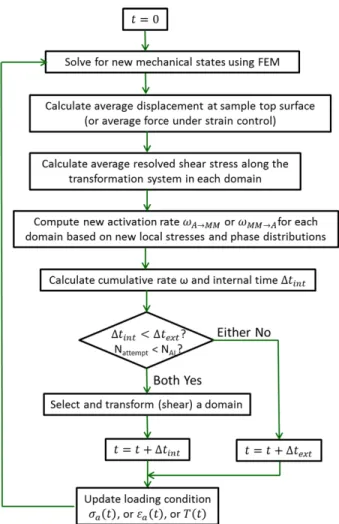
In a standard rejection-free KMC algorithm, an event occurs in every simulation step and the system time t is advanced by Δ . Δ can vary significantly in different steps depending on the phase configuration and activation rates. A very large Δ implies that the system favors the current configuration which does not change until after a long period. Enforcing an event in this case may overextend the system time to beyond the normal duration of experiments or applications, or exclude any possible change in external boundary conditions during this long time interval. To overcome this limitation, we introduce a second time scale referred to as the external time scale Δ . In each simulation step, instead of guaranteeing execution of an event, we determine whether an event will occur by comparing Δ calculated from Eq. (32) to Δ . The simulation procedure flow chart is provided in Fig. 2.
if Δ Δ : Δ and no event occurs
if Δ Δ : Δ and an event occurs (33)
When Δ Δ , no transformation event occurs in this simulation step and the present phase configuration are kept, while the time scale is advanced by Δ . This allows us to update the boundary conditions in a more continuous manner and also capture the critical stresses or temperatures for transformations. Then we move on to the next simulation step when the new stress distributions, activation rates, and ∆ will be calculated, and further compared to Δ .
When Δ Δ , an event occurs and the one to be carried out is selected using the activation rate array as is normally done in KMC. The activation rates for all possible events are strung together to a total length
ω, with each event occupying a distance on the string equal to their individual activation rate, i.e., the
magnitude of → → , or → in Eq. (27) or (29). A second uniform random number ξ2 ∈ (0 1] is generated, and the vector from the origin to a distance along the string points at the event to be executed. Events occupying a large distance along the string (i.e., those with the highest activation rates) thus have a high probability of being chosen. After the transformation event, time is increased by Δ and boundary conditions are updated accordingly. Stress distributions and activation rates of the new phase configuration are then calculated in the next simulation step.
13
Our model setup is illustrated in Fig. 3(a). For ease of implementation in this first incarnation of the model, we limit our attention to a simple two-dimensional specimen under a plane strain assumption; the extension of the approach to three dimensions and more complex geometries is straightforward, if computationally more expensive. Our rectangular simulation cell is subjected to uniaxial tension. Its side surfaces are free without any constraint. Its bottom surface is constrained in the loading direction, while the boundary condition at its top surface is updated in each simulation step using the KMC time t determined in Eq. (33). Under load control with a constant stress ramping rate , the applied uniaxial stress is
| | 0 2 / (34)
We can also run the simulation under a constant strain rate by requiring the uniaxial strain to be
| | 0 2 / (35)
where and are the maximum uniaxial stress and strain, respectively, on the triangular loading curves common in experiments. Therefore transformation behaviors during the entire mechanical cycle including both loading and unloading segments can be simulated by making use of the KMC time. Under thermal cycling, the temperature T first decreases at a constant ramping rate from an initial high temperature to a low temperature , and then returns to . T is assumed to be uniform everywhere in the material, and is varied in each simulation step according to
∆ 0 2 ⁄ (36)
Temperature variation affects the energy barriers → and → in Eq. (25) and also the thermal energy term kT in the rate equations Eqs. (27) and (29). The applied stress can be either kept at zero, in which case thermally-induced transformations are studied, or held at a constant value, which can lead to stress-assisted two-way shape memory effect during thermal cycling.
As shown in the algorithm flow chart in Fig. 2, each simulation step ends with an updated boundary condition. In the next step, finite element analysis determines the new stress states, which are then used to calculate new activation rates and the time increment in KMC. When there is a transformation event, the transformation is a mandatory (stress-free) shear, and the system subsequently relaxes by partitioning and balancing stresses with the surrounding region (which closely resembles an Eshelby inclusion problem). The coupled KMC-FEM algorithm is written as a script, run in the commercial finite element package ABAQUS used as a linear elastic solver.
3.4. Model System and Material Properties
We model a two-dimensional SMA on the mesoscale by hexagonal tessellation. Each hexagonal domain is a phase transformation unit, and only a single domain is involved in each transformation event. The domains are mutually exclusive, because each of them has a phase identity at all times. The simulation
14
cell consists of 1208 domains, and has a width of 33 and a height of about 90 in hexagon edge length. Our code is fairly efficient and for this system size, each simulation step (i.e., an iteration shown in Fig. 2), which includes all the post-processing to extract and analyze stress distributions in the system, takes about twenty seconds on a single quad-core workstation.
The model material is a single-crystalline elastic solid with cubic symmetry. As shown in Fig. 3(a), its [010] direction is oriented 15˚ with respect to the loading axis. We use material properties that are mostly estimated from or reported in the literature for Cu-Al-Ni SMAs, which have extreme elastic anisotropy.
Transformation Crystallography: The transformation shear occurs on {110} planes (habit planes) and along <110> directions [9], sketched as dashed lines in Fig. 3(a). The crystal was intentionally tilted so that the shear directions lie along the lines of symmetry in hexagons.
Shear Strain: The transformations involve little volume change, and in the model they occur by shearwith a simple shear strain 0.1154, which is implemented as pure shear strain 0.5 in the transformation system.
Elastic Constants: The austenite (with cubic symmetry) stiffnesses are = 143.1 GPa, C12 = 124.3 GPa, and C44 = 94.1 GPa [69], which lead to Young’s modulus E ≈ 27.5 GPa, Poisson’s ratio ν = 0.4648, and shear modulus = 94.1 GPa. Note that the modulus for shear in the transformation system is 0.5 , which is only about 9.4 GPa. We assume E and for martensite are the same as those for austenite.
Domain Parameters: By estimation, the material on average has an atomic volume 0.013 nm3 and a vibration frequency 10 /s. Assuming a domain transformation event involves 500 atoms, we assign the transformation characteristic volume Ω 6.5 nm and the attempt frequency 2 1010/s. 3.5. Implementation Strategies(1) Domain Stress Extraction: Each hexagonal domain is meshed with 24 triangular plane strain, 6-node
quadratic elements. From the solved stresses at the three integration points (shown as crosses in Fig. 3(a)) inside each element, we can derive the average resolved shear stress in a domain. However, the non-circular domain geometry gives rise to stress concentrations near edges and corners. For example, Fig. 3(b) shows the shear stress distribution after a domain transforms to martensite when the far-field resolved shear stress 268 MPa, and the shear stresses immediately outside this domain near four of its edges are extremely high (shown in red). In order to exclude such (unphysical) stress concentration spots, we only use the six elements in the center of each domain (highlighted in green in Fig. 3(a)) in the average stress calculations. With this approach, mechanical interactions across phase boundaries can be captured by using a sufficiently small domain size; in principle the domain size should be much smaller than the sample and characteristic scale of the evolving microstructure. (Here we also notice in passing that although 0, the shear stress in martensite is negative (in blue), thereby decreasing the activation
15
energy barrier → for reverse transformation. In the next step there will be competition between reverse transformation of this martensite domain and forward transformation in the remaining austenite domains.)
(2) Boundary Conditions: The boundary conditions applied at the top and bottom surfaces significantly affect
martensite nucleation behavior. Nucleation tends to start in domains near or at the corners of the specimen as these domains are less constrained and experience more elastic relaxation. The specific nucleation site depends on whether the top surface is required to remain flat. When there is no such restriction, the top-right corner would be the most unconstrained spot to transform for transformation shear along [110]. But when the top surface is constrained as a plane, domains near top-left and bottom-right corners are preferential locations because they allow a short band to shear through. Both cases can cause severe local distortion, which may lead to highly irregular and even absurd spatial stress distributions. In order to capture physical responses, a control or buffer layer can be introduced at top and bottom surfaces. The control layers do not undergo transformations, and provide both elastic accommodation and constraint for the transforming material in between. We prohibit the top four rows and bottom four rows of domains from transforming. These domains are set up as austenite initially (i.e., the initial system is a uniform material), but their transformation rates ( → ) are assigned as zero regardless of their local stress state. They never transform as a result, and are effective in promoting side surfaces as nucleation sites and preventing localized severe distortion (which is a direct consequence of boundary conditions). Domains located at the top and bottom of the transformation region no longer experience free surface effects, and this scenario is similar to the response of a sample between grips during uniaxial tension.
(3) Incorporation of Eise: The recoverable energy ∆ as defined in Eq. (11) needs to
be evaluated in each simulation cycle because it appears in the energy barrier expressions in Eq. (25). (i) The surface energy term ∆ is very small and is usually negligible [18].
(ii) The stored elastic energy in the sample, , is incorporated in our simulations implicitly. For example, consider a potential forward transformation in a domain that would result in high stresses in its surroundings and therefore a very high . Instead of raising the energy barrier → to hinder the transformation, our model may allow the domain to transform. But it will likely revert to austenite immediately due to the high driving force for reverse transformation. Therefore, is implicitly incorporated through the effect of the local shear stress
. This approach is computationally much more efficient than determining for each domain, which requires carrying out every possible transformation and calculating the resulting change in the strain energy of the sample.(iii) Therefore, for the present domain-based or unit process approach, for each domain is reduced to , the change in austenite/martensite interface energy, which is incorporated explicitly in each step in the model as it can be determined from the current phase configuration. For an austenite domain surrounded by and austenite and martensite nearest neighbors, respectively,
16
, where is the area (or length in two dimensions) density of each domain boundary. depends on the local phase configuration, which differs from domain to domain and also changes with increasing martensite fraction fM. For an austenite domain with < (this scenario
can emerge at high fM), 0 and it becomes the driving force for martensitic transformation of
this domain, which can lead to a reduction in interfacial area.
(4) Free Surface Effect: Free surfaces can serve as heterogeneous nucleation sites for transformations.
One way to implement surface effect is to introduce into the activation energy barriers in Eq. (24) an energy bias , where As is the domain free surface area density, is the surface defect density,
and is the localized strain energy associated with each surface defect. The term arises from the decreased phase boundary area for transformation at the surface. The term accounts for surface defects, which are often stress concentrators, and increases with increasing surface roughness or defect content. We however choose an alternative approach and directly make use of the local stress bias as described by Eq. (6). This approach deals with surface effect including roughness effect by directly solving for the local stress distributions. Simulation results reported later in Section 4 are obtained from initially smooth (i.e., flat) surfaces, which become serrated during transformation.
(5) Phase Flipping: The algorithm shown in Fig. 2 is efficient because in each simulation step the boundary
condition is updated and/or there is a transformation event. One issue that may cost many simulation steps is the possible occurrence of phase flipping or fluctuation, which can occur during the transformation process in either direction. When there is some sort of metastable phase configuration, the number of martensite domains in the material may switch between N-1 and N and back again in consecutive simulation steps, provided Δ for both the attempted transformation and the backward transformation. As a result, the simulation can spend hundreds and even thousands of steps on such transformation attempts, and Δ in each of these steps can be extremely small. Such frequent attempts within an extremely short period of time seem physical, but do not evolve the phase configuration or the loading condition. To accelerate the simulation, we impose a limit NAL on the number of attempts (e.g., attempt from N-1 to N martensite domains) allowed at each stress level. A transformation event occurs only if Δ Δ and ; otherwise t will be increased by Δ to accelerate the loading condition so that there will be a larger driving force for transformation in subsequent steps.
4. Model Output
In Sections 2 and 3, we laid out the coupled KMC-FEM modeling framework for reversible thermoelastic martensitic transformations in SMAs. The model can be used to simulate a variety of material behavior under various boundary conditions in SMAs. Next, we demonstrate the capability of this model and use it
17
to simulate superelasticity (mechanically-induced transformations) under both load controlled and strain rate controlled loading conditions in single crystal SMAs. Only a limited number of martensite variants are involved because stresses bias towards the favorably-oriented variants over others. As the data to be presented in the following are the first sets of results from this model, we limit our focus here to single-variant behavior in order to clearly illustrate how the model works and what it predicts. Multi-single-variant behavior and inter-variant conversions will be incorporated and addressed in our future work. The simulation results to be presented below therefore only involve transformations between austenite and the martensite variant corresponding to a positive shear on (110)[110] (the 30˚ dashed line in Fig. 3(a)). The following parameter values are used. The temperature T = 300 K. ∆ 3.69 10 J/ , 1.23 10 J/ , and the austenite/martensite interface energy 5 10 J per hexagon edge. The external time scale ∆ 10 s. The loading rate 10 MPa/s when the test is under load control, and the strain rate 5 /s when the test is under strain control. We use an attempt limit NAL = 100 for the present system size (1024 transforming domains).
4.1. Superelasticity at a Constant Loading Rate
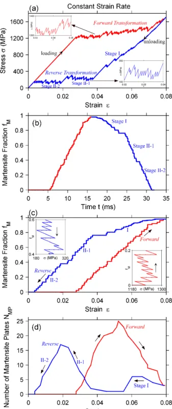
Our model yields superelastic stress-strain curves closely resembling those measured in uniaxial testing experiments. Fig. 4(a) shows a stress-strain curve obtained from simulations performed at a constant loading rate. Upon loading, after a period of elastic deformation, forward martensitic transformation commences; its progression leads to a series of stress plateaus at increasing stresses on the loading curve. During unloading, the stress first decreases rapidly as martensite elastically unloads, although this portion of the unloading curve exhibits subtle serrations caused by some early reverse transformation from martensite back to austenite (Stage I). Succeeding reverse transformation takes place at an almost constant stress (Stage II), but close examination reveals several stress plateaus at decreasing stresses. Complete strain recovery is achieved after unloading.
It is important to note that the present model predicts (rather than enforces) forward and reverse transformations during loading and unloading, respectively. The critical stresses for forward and reverse transformations are model outputs (not input or prescribed), and their magnitudes are dependent on fundamental materials properties (such as the chemical free energy difference ∆ , the frictional work Efr, and the interface energy γi). This model therefore predicts the mechanical response of SMAs based on
their fundamental thermodynamic properties. The hysteresis seen in Fig. 4(a) is large as the present modeling system is a defect-free sample, and it is also related to Efr.
The superelastic curve in Fig. 4(a) exhibits the jerky behavior characteristic of martensitic transformation. The transformations proceed as a series of burst events occurring at different, discrete stress levels. This
18
behavior can also be seen clearly in Fig. 4(b), where martensite fraction fM is plotted as a function of time
t; the slope of this curve yields the transformation rate. The insets in Fig. 4(b) show the temporal evolution
in fM during forward and reverse transformation, respectively, and they both reveal successive episodes of
an abrupt increase (decrease) in fM followed by a period of constant fM. The reverse transformation during
unloading takes place in two stages. A small fraction of austenite gradually reverts to martensite at high stresses (Stage I), and the rest abruptly transforms back to martensite at much lower stresses (Stage II). Fig. 4(c) plots the martensite fraction fM as a function of strain ε. Other than Stage-I reverse transformation,
fM largely increases (decreases) linearly with ε. When transformation occurs at a nearly constant stress,
the elastic strain εe remains unchanged, and the increase in the overall strain ε mainly originates from the
transformation strain εt. For single-variant transformations, , where M is the
Schmid factor and γ0 is the stress-free strain. Using √3/4 and 0.1154 for the present transformation shear system, / 20 . Linear fitting to the data during forward transformation and Stage-II reverse transformation indeed yields 18.844 0.0264 and 20.136 0.0023 , respectively. The small deviations of the fitted slopes, 18.844 and 20.136, from the expected value of 20 results from the minor variations in εe during transformations due to stress changes.
Fig. 4(d) shows how the number of martensite plates, NMP, evolve in a mechanical cycle, and can be compared with the series of snapshots of phase configurations and shear stress distributions in Fig. 5. During forward transformation, NMP first increases from zero to about 24, and this corresponds to the nucleation and formation of new plates. Subsequent transformation proceeds by coalescing existing plates, gradually reducing NMP to 4, driven by a decrease in the total interface energy. During reverse transformation, NMP incurs a small fluctuation before increasing to about 15 and then decreasing to zero, indicating that most of the austenite also forms by developing new plates within martensite and merging these plates. Interface energy contributes to the energy barrier during new plate formation in both forward and reverse transformations, possibly affecting the hysteresis as well.
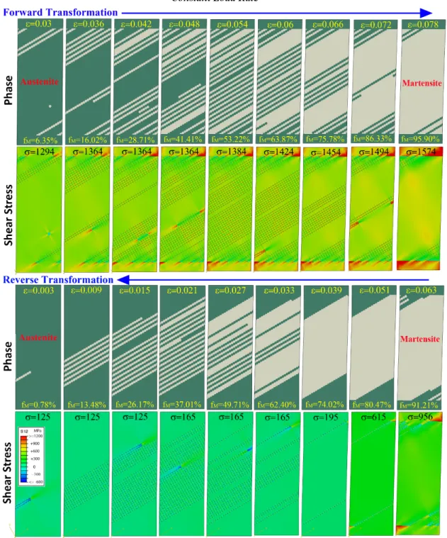
Turning to a closer examination of Fig. 5, the mapped shear stresses are those resolved along the transformation system corresponding to the martensite variant permitted in this simulation. We first examine the austenite-to-martensite forward transformation (top two rows of figures in Fig. 5).
Transformation first started in the upper-left and lower-right corners. As mentioned earlier in Section 3.5, these regions are preferential nucleation sites when the top and bottom surfaces (in the absence of buffer layers) are constrained as a plane. As the buffer layers provide both constraint and elastic accommodation, transformation still initiated in these regions. The partially-transformed metastable band structures in these regions persisted until the highest loads, because the potential reduction in interface energy resulting from further transformation does not outweigh the potential increase in strain energy. The prescribed interface energy γi is relatively low, and these bands are short. The shear
19
stresses in these partially-transformed corner regions are lower than other transformed regions even at high applied loads as can be seen in the stress map corresponding to σ = 1574 MPa.
The regions spanning from the upper-right and lower-left corners completed transformation before the center of the sample did. The strain energy penalty for transformation in these regions might be lower due to the accommodation effect of the buffer layers, which can deform severely (as reflected by the high stresses) near these two corners as the side surfaces are not constrained.
The main mechanism controlling forward transformation is nucleation, leading to a band structure with a few different band widths, which is commonly seen in experiments. Although nucleation tends to occur at surfaces, it occasionally takes place inside the sample as can be seen at ε = 0.042 and 0.048. These interior martensite bands then grow outwards in both directions and reach the surface. This behavior might be explained by the low interface energy γi as well as the small size of the present
system in which interior domains also experience some surface relief. The presence of a neighboring martensite band could also facilitate this behavior, since an alternating band structure is a low strain energy configuration. The transformation might also involve some interface propagation, such as the mode by which the austenite band in the sample center at ε = 0.072 shrinks.
We next analyze phase changes and stress evolution during martensite-to-austenite reverse transformation (bottom two rows of figures in Fig. 5).
The upper-left and bottom-right corner regions, which retained some austenite, completed reverse transformation first (corresponding to Stage-I reverse transformation on the stress-strain curve in Fig. 4(a)). As the applied stress decreases, martensite in these regions becomes less and less favorable because of even lower local stresses. Reverse transformation in these regions is further motivated by the elimination of existing interfaces between martensite and retained austenite. As shown in the figures corresponding to ε = 0.063, 0.051, 0.039, and 0.033, austenite in these regions clearly grows by interface propagation and reaches a relatively stable elongated-wedge phase geometry at ε = 0.051 and σ = 615 MPa. The rest of these corner regions did not transform until the uniaxial stress was lowered to below 200 MPa.
After reverse transformation in the corner regions completed, the sample center started reverting to austenite, mainly by nucleation of austenite and formation of a band structure, at σ = 165 MPa. Later on, interface propagation is also observed (e.g., when eliminating the wider martensite band at ε = 0.021).
For both forward and reverse transformations, once a plate is nucleated, it grows rapidly because very high positive/negative stresses develop at the martensite/austenite transformation front. Further transformation after a band structure with alternating phases is achieved (i.e., after reaching a maximum NMP in Fig. 4(d)) requires a much higher driving force, i.e., much higher/lower stresses during forward/reverse transformation.
20 4.2. Superelasticity at a Constant Strain Rate
In Section 4.1, we presented simulation results from a constant load rate test, during which most of the time was spent on elastic loading and unloading and only a short period on phase transformations. Under a constant strain rate, the transformation should occur more gradually over a longer period of time because transformation strain increases linearly with martensite fraction. This boundary condition is used frequently in experimental studies that explore rate effects in SMAs [9, 63, 70, 71], and also allows us to capture possible stress relaxation behavior.
A superelastic stress-strain curve obtained from strain-controlled simulations is presented in Fig. 6(a), along with snapshots of the phase evolution in Fig. 7. The input parameters used are the same as those used in the load-controlled simulation results shown in Figs. 4 and 5. As a result, the predicted critical transformation stresses in the two cases are similar, and so is the average stress hysteresis. What is different is how the stress evolves. Frequent stress fluctuations are seen during both forward and reverse transformations in Fig. 6(a). The insets in Fig. 6(a) are close-up views of the stress-strain curve, showing sudden stress drops (rises) during forward (reverse) transformation, each followed by a period of elastic loading (unloading) with a slope parallel to that of the initial elastic loading curve.
Numerous small serrations are seen in both Fig. 6(b) and (c), where martensite fraction fM is plotted as a
function of time t (in milliseconds) and strain ε, respectively. fM actually increases or decreases by a small
percentage at a constant ε, and then pauses over a range of ε before increasing or decreasing at another constant ε. The insets in Fig. 6(c) show how the overall external stress σ changes with fM. During forward
transformation, the increase in fM always results in a decrease in σ, which subsequently increases at a
constant fM. Therefore with increasing applied strain, strain increment is first achieved by elastic
deformation of the sample, leading to an increase in σ and a reduction in the free energy of martensite, GM.
Subsequently, martensitic transformation occurs in some regions of the sample and the resulting transformation strain fulfills the strain increment requirement, leading to relaxation of the elastic stress developed prior to transformation. Stress relaxation has indeed been observed in tensile testing of small SMA microwires under a constant slow strain rate [70]. During reverse transformation, the decrease in fM
always leads to an increase in σ, which subsequently decreases at a constant fM. Strain reduction is first
realized by elastic unloading, which in turn raises the driving force for reverse transformation. Eventually reverse transformation takes place, meeting the strain reduction requirement by the recovered transformation strain. The stress rises rapidly and then the next iteration begins.
In general, forward transformation is similar to that in load-controlled simulations. Its progression drives the overall stress up, and causes the number of martensite plates, NMP, to increase to a maximum of 25 and then decrease to 3 (Fig. 6(d)). Overall, martensite fraction fM still seems linearly related to strain ε (for
21
example, linear fitting of the forward transformation data in Fig. 6(c) yields 20.61 0.0268 ), but a linear relationship is no longer accurate because fM increases in a discontinuous manner. Reverse
transformation still takes place in two stages, Stage-I occurring at high stresses and Stage-II at much lower stresses. However, Stage-II transformation now further separates into two distinct overall stress levels, Stage II-1 and Stage II-2, separated by a relatively long period of elastic unloading (see Fig. 6(a)). The transition point corresponds to a large reduction in ε near ε = 0.2 at a constant fM in Fig. 6(c)), and to the
maximum NMP during reverse transformation in Fig. 6(d). New austenite plates form at stresses fluctuating around 250 MPa, but coalesce at stresses below 150 MPa.
Maps in Fig. 7 have the same martensite fraction fM as those in Fig. 5. In contrast to the load-controlled
simulation results in Fig. 5, martensitic transformation now starts in the center (rather than the ends or corner regions) of the sample. Under a constant strain rate, formation of long plates that span across the sample leads to a higher overall transformation strain and more stress relaxation compared to shorter plates at corner regions that are constrained by the buffer layers. The corner regions partially transformed at higher strains (e.g., ε = 0.04-0.052), and retained some austenite until very high applied strains. The transformation behavior near the corner regions resembles that in oligocrystalline SMA wires with a bamboo grain structure [72]; the buffer layers in the present simulations may play a similar role as unfavorably oriented grains that do not transform within the range of applied load. In other regions, new martensite plates formed at relatively low strains and grew and impinged at higher strains. Phase development during this process is similar to those seen in Fig. 5, but the stress evolution is no longer monotonic. Formation of a martensite plate usually leads to extensive stress relaxation. During unloading, the corner regions reverted to austenite first, but exhibited slightly less propagation behavior compared to the load-controlled case shown in Fig. 5. Again the phase evolution during reverse transformation is similar to that in Fig. 5, but formation of austenite plates results in stress spikes.
In summary, the present model yields superelastic stress-strain curves with complete strain recovery under both load-controlled and strain-controlled boundary conditions. It also captures the salient features of the incubation, nucleation, and growth processes of martensite and austenite. Although the computational examples shown in this section use simple two-dimensional single crystal samples that involve a single martensite variant, the model can incorporate multi-variant behavior as well as more complex sample geometries and microstructures. When multiple variants are involved, the local resolved shear stress on the transformation system of each variant needs to be calculated, and the cumulative rate needs to be determined from Eq. (30) that incorporates inter-variant conversions. Extension to polycrystalline systems requires identification of transformation shear planes and directions in each grain. When the problem is extended to three dimensions, domain geometry will be more complicated and there will be a larger number of variants. In this section we have demonstrated that this model can be used to simulate superelasticity, but it can also be utilized to study one-way and two-way shape memory effects. During cooling or heating,
22
the free energy difference between the two phases, ∆ , changes as described in Eq. (5). The resulting changes in activation energy barriers for transformations ( → and → in Eqs. (24) and (25)) provide driving force for thermally-induced transformation that gives rise to shape memory effects. There are many possible future applications of this new mesoscale modeling tool.
5. Conclusions
We have developed a coupled kinetic Monte Carlo-Finite Element (KMC-FEM) mesoscale dynamics model for thermoelastic and reversible martensitic transformations in shape memory alloys. Martensitic transformation occurs by a mandatory displacement which is mainly a shear, and is modeled as a unit process that takes place in one domain at a time. After each domain transformation event, the boundary conditions are updated according to the new time scale and the new stress states in the sample are calculated by FEM. The new phase configuration and stress distributions are used to determine the activation rate for each domain based on a transition state approximation for the energy landscape of the transformation states. We then use the KMC algorithm to select the next domain to transform and determine the time increment. This iterative KMC-FEM simulation method therefore performs virtual in-situ testing, and predicts simultaneous phase and stress evolution in the sample using physical time and length scales comparable to those involved in experiments. It in particular captures transformation stochasticity. This paper lays out the theoretical and computational framework for this new KMC-FEM mesoscale model. The thermodynamic energetics governing austenite↔martensite transformations induced by both temperature changes and applied stresses are examined, and the energy landscapes for phases and for transformation states are developed. Thermodynamics is connected to kinetics through a rate equation that is commonly used to describe thermally-activated phenomena. KMC provides FEM a new phase distribution as well as a new time scale (and thus new boundary conditions). The results from FEM in turn lead to changes in the energy landscape for the transformation states. Computational implementation of the model is realized and presented.
We have demonstrated the capability of the model by using it to simulate superelasticity (mechanically-induced reversible transformation) under both constant loading rate and constant strain rate conditions, for single-variant transformation conditions in plane strain two-dimensional specimens. The model predicts phase and stress evolution during the entire incubation, nucleation, and growth process of the new phase. It also predicts (rather than enforces) both forward and reverse transformations, and the predicted critical transformation stresses are related to fundamental thermodynamic properties of materials. For the set of simulation parameters used, both boundary conditions yield stress-strain loops and complete strain recovery characteristic of superelasticity; the number of martensite plates first increases and then
23
decreases during transformations in both directions. Stress relaxation and spikes are observed during transformations under a constant applied strain rate.
This modeling tool could significantly augment mesoscale computational materials/mechanics capabilities that connect microstructures to macroscopic thermomechanical properties. While the sample used in the examples illustrated in this paper is a defect-free single crystal, the model is capable of capturing transformation-microstructure interactions and addressing issues of transformation kinematics in the presence of defects. Although the model is currently developed for reversible martensitic transformations in shape memory alloys, it can also be adapted to study the broad class of materials that are susceptible to microstructure changes under thermal, mechanical, or combined stimuli, such as other phase change materials, far-from-equilibrium materials, and materials used in extreme environment applications.
Acknowledgments
Y. Chen acknowledges the support from the US National Science Foundation with award number DMR-1352524 as well as the RPI start-up support. Y. Chen is grateful to Dr. E.R. Homer (formerly with MIT and currently with BYU) who provided helpful discussions. C.A. Schuh acknowledges the support of the US Army Research Office through the Institute for Soldier Nanotechnologies (ISN) at MIT.
24
References
[1] Lagoudas DC. Shape Memory Alloys: Modeling and Engineering Applications: Springer, 2008. [2] Tadaki T, Otsuka K, Shimizu K. Annu Rev Mater Sci 1988;18:25.
[3] Karaca HE, Karaman I, Basaran B, Lagoudas DC, Chumlyakov YI, Maier HJ. Acta Materialia 2007;55:4253. [4] Otsuka K, Wayman CM. Shape Memory Materials: Cambridge University Press, 1998.
[5] Otsuka K, Sakamoto H, Shimizu K. Acta Metall 1979;27:585.
[6] Ibarra A, Caillard D, Juan JS, No ML. Appl Phys Lett 2007;90:101907. [7] Wollants P, Roos JR, Delaey L. Progr Mater Sci 1993;37:227.
[8] Koeda N, Omori T, Sutou Y, Suzuki H, Wakita M, Kainuma R, Ishida K. Mater Trans 2005;46:118. [9] Otsuka K, Wayman CM, Nakai K, Sakamoto H, Shimizu K. Acta Metall 1976;24:207.
[10] López del Castillo C, Mellor BG, Blázquez ML, Gómez C. Scripta Metall 1987;21:1711. [11] Seki K, Kura H, Sato T, Taniyama T. J Appl Phys 2008;103.
[12] Araya R, Marivil M, Mir C, Moroni O, Sepúlveda A. Mater Sci Eng A 2008;496:209. [13] Sutou Y, Omori T, Koeda N, Kainuma R, Ishida K. Mater Sci Eng A 2006;438:743. [14] Frick CP, Orso S, Arzt E. Acta Mater 2007;55:3845.
[15] Juan JMS, No ML, Schuh CA. Adv Mater 2008;20:272.
[16] Norfleet DM, Sarosi PM, Manchiraju S, Wagner MFX, Uchic MD, Anderson PM, Mills MJ. Acta Mater 2009;57:3549.
[17] Juan JS, No ML, Schuh CA. Nat Nanotech 2009;4:415. [18] Chen Y, Schuh CA. Acta Mater 2011;59:537.
[19] Boonyongmaneerat Y, Chmielus M, Dunand DC, Müllner P. Physical Review Letters 2007;99:247201. [20] Chmielus M, Zhang XX, Witherspoon C, Dunand DC, Mullner P. Nature Materials 2009:DOI:10.1038/nmat2527.
[21] Ueland SM, Schuh CA. Acta Mater 2012;60:282. [22] Zhu JJ, Liew KM. Acta Mater 2003;51:2443.
[23] Bowles JS, Barrett CS. Crystallography of Transformations: Pergamon Press, 1952. [24] Mackenzie JK, Bowles JS. Acta Metall 1954;2:138.
[25] Chakravorty S, Wayman CM. Metall Trans A 1976;7:555. [26] Gupta SK, Raghavan V. Scripta Metall 1974;8:901.
[27] Grujicic M, Olson GB, Owen WS. Metall Trans A 1985;16:1713. [28] Grujicic M, Olson GB, Owen WS. Metall Trans A 1985;16:1735. [29] Pond RC, Hirth JP. Philosophical Magazine 2010;90:805. [30] Pond RC, Celotto S, Hirth JP. Acta Mater 2003;51:5385.
[31] Yang JB, Yang ZG, Nagai Y, Hasegawa M. Acta Mater 2010;58:1599. [32] Olson GB, Cohen M. Scripta Metall 1975;9:1247.
[33] Fisher JC, Turnbull D. Acta Metall 1953;1:310.
[34] Klein W, Lookman T, Saxena A, Hatch DM. Physical Review Letters 2002;88:085701. [35] Ortín J, Planes A. Acta Metall 1989;37:1433.
[36] Ortín J, Planes A. Acta Metall 1988;36:1873.
[37] Huo Y, Müller I. Continuum Mech. Thermodyn 1993;5:163. [38] Falk F. Acta Metall 1980;28:1773.
[39] Auricchio F, Sacco E. International Journal of Solids and Structures 2001;38:6123.
[40] Tadashige I, Florin Andrei N, Hisashi N, Yuji M. Smart Materials and Structures 2004;13:916. [41] Sun QP, He YJ. International Journal of Solids and Structures 2008;45:3868.
[42] Planes A, Ortín J. J Appl Phys 1992;71:950.
[43] Zhu JJ, Liang NG, Cai M, Liew KM, Huang WM. Smart Materials and Structures 2008;17:015041. [44] Lu ZK, Weng GJ. Journal of the Mechanics and Physics of Solids 1997;45:1905.
[45] Tatar C, Kazanc S. Current Applied Physics 2012;12:98.
[46] Kastner O, Eggeler G, Weiss W, Ackland GJ. Journal of the Mechanics and Physics of Solids 2011;59:1888. [47] Zhong Y, Gall K, Zhu T. Acta Mater 2012;60:6301.
[48] Guda Vishnu K, Strachan A. Phys Rev B 2012;85:014114.
[49] Ozdemir N, Karaman I, Mara NA, Chumlyakov YI, Karaca HE. Acta Mater 2012;60:5670.
[50] Gall K, Lim TJ, McDowell DL, Sehitoglu H, Chumlyakov YI. International Journal of Plasticity 2000;16:1189. [51] Wood AJM, Clyne TW. Acta Mater 2006;54:5607.
[52] Gall K, Sehitoglu H. International Journal of Plasticity 1999;15:69.
[53] Patoor E, El Amrani M, Eberhardt A, Berveiller M. J. Phys. IV France 1995;05:C2. [54] Manchiraju S, Anderson PM. International Journal of Plasticity 2010;26:1508.
[55] Manchiraju S, Gaydosh D, Benafan O, Noebe R, Vaidyanathan R, Anderson PM. Acta Mater 2011;59:5238. [56] Jin YM, Artemev A, Khachaturyan AG. Acta Mater 2001;49:2309.
[57] Mamivand M, Asle Zaeem M, El Kadiri H, Chen L-Q. Acta Mater 2013;61:5223. [58] Mamivand M, Asle Zaeem M, El Kadiri H. Acta Mater 2014;64:208.