Correlations in Firm Default Behavior
by
Sreeram Thirukkonda
S.M., Massachusetts Institute of Technology (1997)
Submitted to the System Design and Management Program
in Partial Fulfillment of the Requirements for the degree of
Master of Science in Engineering and Management
at the
MASSACHUSETTS INSTITUTE OF TECHNOLOGY
June 2009
@ Massachusetts Institute of Technology 2009
All rights reserved.
Author ...
ARCHVES
MASSACHUSETTS INSTITUTE OF TECHNOLOGYSEP 2 3 2009
LIBRARIES
/
.., - ...
Sreeram Thirukkonda
System Design and Management Program
May 2009
Certified by ...
Accepted by ...
Scott Joslin
Assistant Professor of Finance
MIT Sl n School of Management
(k'arick Hale
Director
System Design and Management Program
Correlations in Firm Default Behavior
by
Sreeram Thirukkonda
Submitted to the System Design and Management Program on May 2009, in Partial Fulfillment of the
Requirements for the Degree of
Master of Science in Engineering and Management
Abstract
Modeling credit risk using Structural and Reduced Form models has been a popular and apropos topic of research. This work makes an attempt to better understand correlations in firm default. A review of contemporary research reveals several models with varying degrees of assumptions around firm default and how they relate to macro-economic variables. More recent literature also makes use of a doubly stochastic assumption which in essence holds that given a certain path of covariates the default probabilities of two similar firms is independent. We explore empirical evidence which points to correlated defaults conditional on various explanatory covariates. Given the strong similarities in underlying firm structure and relationship to macro-economic environment, it can be hypothesized that there exist correlations in default behavior among similar firms.
Thesis Supervisor: Scott Joslin Title: Assistant Professor of Finance
Acknowledgments
It is my pleasure to take this opportunity to convey my gratitude to all the people who have contributed to this thesis in many different ways.
This work would not have been possible without the knowledge and guidance of my advisor, Dr. Scott Joslin. In addition to providing insightful comments, invaluable computing resources and beneficial data pointers, his immediate responses even on weekends, helped me make steady progress. I also greatly appreciate his flexibility with schedules and willingness to work with my part-time schedule.
I express sincere appreciation and thanks to Mr.Thomas Linkas, CIO Battery-march,for his periodic reviews. Through his finance acumen and experience, he was able to provide insights which accelerated research efforts and helped anticipate prag-matic limitations in financial data.
I am deeply indebted to Dr.Yoonjung Lee, Faculty of the School of Statistics, Harvard University. Her stimulating discussions, ideas and comments helped bring together the alternate model structures.
I am pleased to acknowledge the flexibility provided by Dr. Patrick Hale and the SDM program without which I could have not gathered enough background for this work.
Finally, I express my special thanks and appreciation to my wife for her endless patience, encouragement and support that enabled me to complete this work.
Contents
1 Introduction
1.1 Literature Review . ... 1.1.1 Structural Models . ...
1.1.2 Performance of Structural Models . 1.1.3 Reduced Form Models ... 1.1.4 Hybrid Models ...
2 Model Framework
2.1 Base Model Definitions . ... 2.1.1 Doubly Stochastic Hybrid Model 2.1.2 Correlations in Corporate Default .
3 Analysis of Correlation in Corporate Default 3.1 Basic Definitions ...
3.2 Data Description ... 3.3 Proposed Tests and Results ...
4 Technical Architecture and Data Overview
4.1 COMPUSTAT Data Feed ...
4.1.1 The COMPUSTAT/CRSP Merged format 4.1.2 Alternate Data Sources ...
4.2 Technical Architecture ...
4.2.1 System components . ...
7
4.2.2 Database tables: Data from Finance Sources ... . . . 38
4.2.3 Database tables: Generated Data ... ... . 39
4.2.4 Generating Estimation Inputs ... ... 41
5 Model Extensions and Results 45 5.1 Introduction ... ... 45
5.2 Model Calibration. . ... ... 46
5.2.1 Econometric Background for Model Calibration ... . 46
5.2.2 Constrained Minimization to Optimize the Likelihood .... . 47
5.3 Results and Interpretations ... ... ... ... 48
5.3.1 Reduced Form model for Default Intensities . ... 48
5.3.2 Applying Models to Recent Periods ... . ... .... 57
5.4 Study of Correlation Metrics . ... . . ... 58
5.4.1 Comparison with Other Contemporary Models ... . . 59
6 Summary 63 6.1 Model Extensions and Results ... ... .. ... 63
6.2 Future Extensions . .. ... ... .... 64
A Tables 69
List of Figures
2-1 Comparison of Distance to Default vs. Altman Z-score ... ... 23
3-1 Log Change in Industrial Production ... . ... 31
3-2 Smoothed Log Change in Industrial Production ... . ... . 31
4-1 Distribution of Days between End of Price and Default Date . .... 43
4-2 Actual observed defaults in various sectors between 1980 to 2004 . . . 44
5-1 Optional caption for list of figures ... ... . . ... 49
5-2 Actual Counts vs. Predicted Aggregate Intensities . ... 51
5-3 Optional caption for list of figures ... .. . . ... ... 53
5-4 Actual Counts vs. Predicted Aggregate Intensities . ... 54
5-5 Comparison of Default Intensity Prediction . ... ... 55
5-6 Comparison of Aggregate Counts vs. Predicted Intensities ... 55
5-7 Actual Counts vs. Predicted Aggregate Intensities . ... 57
5-8 Comparison of Default Intensity Prediction . ... .. 57
5-9 Comparison of Aggregate Counts vs. Predicted Intensities . .... . . 58
5-10 Optional caption for list of figures ... ... ... 60
B-1 Moodys KMV Annual Report on Default Intensities 1920-2008 . . . . 72
B-2 Model Parameters from Duffie et al ... .. .... . ... 73
List of Tables
2.1 Altman Z-Score . . ... ... . 23
3.1 Time-based Bins: Summary Statistics for Bin Size=8 ... . . 32
3.2 GIP-based Bins: Summary Statistics for Bin Size=8 ... . 32
5.1 Increase in Exit Types 2006-2008 ... ... ... 58
5.2 Correlation Metrics from the Models, Time Binning, Size=8 .... . 59
5.3 Correlation Metrics from the Models, GIP Binning, Size=8 ... 59
5.4 Correlation Metrics, Bin Size=8, Model 3, 1980-1993 . ... 60
5.5 Correlation Metrics, Bin Size=8, Model 3, 1994-2004 . ... .. 61
5.6 Parameters for the two time period models ... .... ... . .. 61
Chapter 1
Introduction
Credit risk is a significant concern to most financial institutions. Given recent events, this is probably as applicable to regulators as it is to institutions. Institutions spend considerable resources to manage and develop various measures of credit risk in their portfolios. Risk measures can be computed on a per portfolio basis or computed to measure the total risk to which a financial institution is exposed in the market. Credit risk constitutes an important category of risk which institutions seek to mitigate. By definition, it arises from the fact that borrowers or lenders on either side of a financial transaction can default. Credit risk modeling has been and continues to be an active area of research. The two broad class of models dealing with credit risk are Structural Models and Reduced Form models.
This introduction deals with these two broad classes of models and examines the inherent tradeoffs associated with each type. Subsequently, significant milestone models of each category are examined leading up to hybrid models which try to incorporate the best of both worlds.
Chapter Two attempts to provide a high level holistic view of the various sig-nificant subsystems and mechanisms which depend upon credit risk modeling. A broad-based systems dynamics framework has been used to illustrate the various
un-derlying relationships.
Chapter Three describes the modeling framework used in the current work for these hybrid class of models. Key model assumptions as well as earlier work are also
examined.
Chapter Four discusses the data used within the current work including sources, formats and additional constraints. This chapter also includes an overview of the tools and platforms used in data analysis as well as a description of the real and simulated data inputs.
Chapter Five outlines the Key Learnings & Outputs from the models developed in Chapter Three. In addition, interpretations are offered for key model findings in the context of data from financial statements.
1.1
Literature Review
1.1.1
Structural Models
Merton's Model
Black and Scholes (1973) [9] and Merton (1974) [22] revolutionized credit risk mod-eling by introducing models of Corporate Liabilities. The class of models referred to as structural models were launched through these seminal efforts. One of the key assumptions of structural models is that of a complete information set very similar to that known to corporate finance managers. This information is also assumed to be perfect and to incorporate market perception of the firm.
Merton proposed that a firm's equity could be considered as a option on the underlying assets of the firm. The total underlying assets equals the sum of the total debt and total equity of the firm. Hence the debt level could be treated analogous to the strike price of the equity option. Within this framework, a company whose assets fall below the debt level would be considered to be in default. A default event would wipe out the equity holders while protecting the debt holders to the extent to which assets can be liquidated and recovered. Under this framework, the following results are well known and have been extended in numerous ways:
Eo = VoN(dl) - De-'TN(d2) (1.2)
di
= ln(Vo/D) + (r + u2/2)T d2 d - vVT (1.3)
cy T , d2 = Cd - uv (1.3)
Also, from Hull [12] applying Ito's lemma to the above,
dE
E Eo = av Vo (1.4)
OV
EEo = N(dl)acvVo (1.5)
Extensions of the Merton's Model
Barrier Levels Merton's model assumes that the zero equity level triggers the firm to go into bankruptcy. However, in reality, firms are subject to various bond safety covenants which specify debt to equity ratios that need to be maintained above a predetermined level in order for the firm to exist. Hence, firms are forced into default through such covenants which translate effectively to a non-zero default boundary applied to the Merton's model. Black and Cox (1976) [8] extended the Merton's model to incorporate such boundaries. They define a time dependent boundary as follows:
L(t) = Ce- (T- t ) (1.6)
Noting that the above form allows for the boundary level to be analogous to the definition of asset level in the classic Merton model, an analytical solution can be obtained. With a non-zero boundary, in the Black-Cox model any residual positive assets below the boundary are transferred to the bond holders.
Vasicek-Kealhofer model Vasicek and Kealhofer, in a collection of works [17], [23], [24] and [15], extended the basic Merton model and included items from the
firm's balance sheet in order to incorporate better information from the firm's financial accounting statements. This model was further enhanced into the Expect Default FrequencyTMor EDF credit measure TM .This approach built upon an earlier Moodys
KMV notion of distance to default which was defined as
In(VT/D) + - /2)T(1.7)
where the default point D was defined as (0.5 x (long term debt) + short term debt) while the rate of return on the firm is defined as the expected value of the rate of asset growth or
S= E(1n(Vt/Vt_i)) (1.8)
Other variants of Merton's model Longstaff and Schwartz (1995) [10] intro-duce stochastic interest rates to augment the basic Merton model into a two factor specification. The essence of this model is as follows:
dV(t) = r(t)V(t)dt + rvV(t)(p * dW(t) + 1 - p2dW2(t)) (1.9)
dr(t) = K(O - r(t))dt + r,dW2(t) (1.10)
where W1 (t) and W2(t) are two independent Brownian Motions
However, in practice it has been observed that interest rates have to be very volatile in order to have an impact on credit spreads. This insensitivity is used by researchers to support arguments ignoring the effect of stochastic interest rates on the credit spreads. The correlations between interest rates and asset values appear to play a stronger role. As asset values fall when the rate of economic activity slows down, typically so do the interest rates. This strengthens the drift of the underlying assets pushing them closer to bankruptcy. Lyden and Saraniti (2000) [25] also confirmed this finding.
Collin-Dufresne and Goldstein (2001) [16] extend the Longstaff model by intro-ducing a stationary leverage ratio allowing firms to deviate from their target leverage ratio.
1.1.2
Performance of Structural Models
Several of these model extensions of the underlying Merton model are still being tested. It has been observed by Eom et al. (2000) [6] that structural models tend to over-predict the spreads for risky firms with high leverage. On the other hand Ogden (1987) [18] concluded that, for safer firms, they tend to under-predict the spreads. In either case, the computed spreads are conditional on the firm having survived. Structural models are also found to be insensitive to interest rate variations. Structural Models are founded on the assumption of a perfect information set typically known to corporate finance managers. In more recent times with several accounting mishaps, this appears to be questionable at best. In addition, the availability of alternate attractive market pricing mechanisms such as credit default swaps have prompted researchers to migrate towards a flexible and mathematically tractable framework.
1.1.3
Reduced Form Models
Reduced Form models assume an imperfect information set and that market variables can be used to predict default events. For reasons discussed in the last section, this family of models has been gaining traction since the late 90s. Reduced Form models assume that a firm's default time is inaccessible and driven by a default intensity which is determined by latent state variables.
Jarrow, Lando and Turnbull (1995) [21], Duffie and Singleton (1999) [3], Hull and White (2000) [13] and Jarrow and Protter (2004) [20] present different Reduced Form models and argue within an information theoretic context that one is unlikely to have complete information about the firms default intensity or the recovery rate. Assuming that the financial modeler only has as much information as the market appears to be more realistic.
In addition, Structural Models appear to be simplified representation of the eco-nomic nuances of a firm's operation. This has been observed in numerous occasions in more recent times in which a firm's financial statements are loaded with Off Balance
Sheet assets and liabilities which are hard to observe, quantify and incorporate into the Merton model.
The following definitions are common to most works dealing with Reduced Form Models. The default intensity At is defined such that the probability of default in interval dt is Atdt. Hence, the conditional probability of survival through time t + dt given that the firm has survived through time t is as follows:
Vt+dt = Vt(1 - Atdt) (1.11)
Extending this notion, the conditional probability of default under the risk-neutral measure can be derived as follows:
Q(T > T) = EQ[efoT (X(s))ds] (1.12)
where the default intensity can be expanded as below where each of the X, cor-respond to latent explanatory state variables.
A(X(s)) = elO+mX° + ...+X - " (1.13)
Only statistical significance limits the choice of latent variables which can be used to explain the default intensity. Both firm-specific and global variables are typically used. The flexibility of these models is a double-edged sword. Although these models are clearly mathematically tractable, the lack of economic interpretation can be a drawback. Duffie and Singleton [11] also show that bond prices used as latent variables in such models can reduce the usefulness of these models if they are restricted to indicative bond data. Hence, when Reduced Form models are used to predict defaults, it is important to consider incorporating prices which are close to transaction prices i.e. as real time as can possibly be obtained. However, such data sources are relatively new and can be hard to obtain.
Jarrow and Protter [20] also point out that with Reduced Form models, model portability and separating model quality from data issues can be a problem. Closely related is the issue of model performance in out of sample data sets.
1.1.4
Hybrid Models
More recently, modelers have also attempted to incorporate the Information Content of Structural Models into the tractable framework of Reduced Form models. Hence this class of models tries to bring together the best of both worlds by devising latent variables from outputs of the Structural Models. Duffie, Saita and Wang [5] present one such model which draws upon the Merton's Structural Model enhanced with Balance Sheet items to compute the Distance to Default. This variable is then used as a covariate in the default intensity computation.
The distance to default can be defined as follows:
log V/Lt + (IPA - 0.5 * o~)T
Dt = (1.14)
JAT
In this expression, the PA and OA measure the firm's mean rate of asset growth and asset volatility. Vassalou and Xing (2004) [26] and [19] establish the default point
Lt from balance sheet items such as short-term debt and long-term debt.
Similarly, the modeler is free to choose other variables as suitable covariates in the expression for the default intensity. Duffie, Saita and Wang [5] use the Security returns, the 3 month treasury bill rate and the Standard and Poor's 500 Index return as covariates.
Chapter 2
Model Framework
2.1
Base Model Definitions
2.1.1
Doubly Stochastic Hybrid Model
One of the base models studied in this work was originally proposed by Duffie et al. [5]. As discussed in Chapter 1, this model is a hybrid model which incorporates elements from both Structural and Reduced Form models.
Also as previously discussed, Structural Models provide useful economic interpre-tations and valuable insights into the capital structure of firms and how it can change with significant equity-raising or debt reducing actions. Reduced Form Models, on the other hand, are mathematically tractable and allow for several different latent variables to be incorporated into the model to allow the capture of any incremental information. Hybrid Models borrow latent variables from structural models and use them as part of a Reduced Form expression. This allows the use of extended Struc-tural Variables such as Distance to Default and Expected Default Frequency into a Reduced Form expression. In addition, modelers are free to choose other variables which can lend additional insights.
The base model consists of the covariates defined by Duffie et al. [5]. This model has a hybrid form which incorporates both firm specific and global covariates. The underlying structure is that of a Reduced Form model which consists of the Distance
to Default and the Security Returns as the firm specific covariates. In addition, the model also consists of the three month treasury bill rates and the S&P 500 returns as global covariates.
Distance to Default
There is ample research on computing Distance to Default in various ways. The original definition of distance to default, as developed by Merton is as follows:
D n(VA/D) + (r - - t)))(T
DDMerton (2.1)
erton A -t
This amounts to roughly the number of standard deviations by which the firm's value is from the default point. The higher the distance to default, the more likely the firm is to default. This distance to default can also be mapped naturally to a probability of default. An alternate simpler method to compute the distance to default was introduced by Bystorm [2]. In this work, the author argues that, with some simplifying assumptions, the Merton model can be used to yield a simpler expression for distance to default. The author defines this measure as follows:
In(1/L)
DDsimplified Merton =_E( L) (2.2)
UE (1 - L)
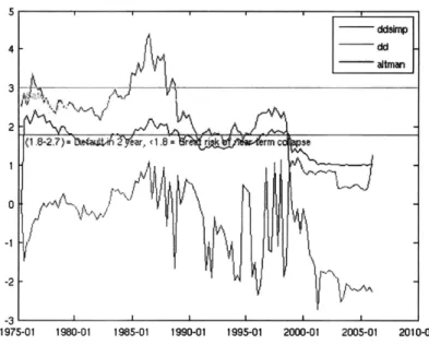
In the expression above, L = D/(D + VE) is the leverage ratio in which D is the total debt and VE stands for the market value of the total equity of the firm. Also to be noted in the above expression is that aE is the volatility of the equity which can be computed in numerous ways ranging from simple equity based measures to GARCH or stochastic volatility. In order to measure the effectiveness of the simplified distance to default, this research studied the effectiveness of this measure against that of the traditional measure for a few real-life default scenarios. It appears that, although this model reflects the trend of the DD,,t,,, it tends to underestimate the magnitude of the underlying distance to default. A few summary plots of this measurement are shown below.
3 ---- --
---.1-2.7)8-=2. bW 4 2 , <1.8 r S r rn mo
-2
-3
1975-01 1980-01 1985-01 1990-01 1995-01 2000-01 2005-01 2010-01
Figure 2-1: Comparison of Distance to Default vs. Altman Z-score
Table 2.1: Altman Z-Score
Term Ratio Constant
A EBIT/Total Assets 3.33
B Net Sales/Total Assets 0.99
C Mkt Val of Equity/Total Liabilities 0.60 D Working Capital/Total Assets 1.20 E Retained Earnings/Total Assets 1.40 Z-Score = 3.33xA+0.99xB+0.6xC+1.2xD+1.4xE
a popular measure which is typically used as a proxy for the firm's financial health by researchers, analysts and modelers. The expression for the Z-score and additional background can be found at http://en. wikipedia. org/wiki/Z-Score_Financial Analysis_Tool. The structure of the Z-Score is shown in Table 2.1.
The plot shows the comparative performance of the three measures for a sample firm in default.
The base model used by Duffie et al. circumvents the need to calculate aE by using a modified expression for the distance to default. This uses an approach which appears to combine those introduced by Vassalou et al. [26] and Vasicek-Kealhofer
[23]. Vassalou et al. use an iterative method to simultaneously calculate the market value of a firm's assets and the underlying volatility of the assets. In addition, the mean rate of return of the firm is computed as the rate of growth of the firm's assets
and the volatility of the assets is assumed to be the Standard Deviation of the rate of growth of the firm's assets. The following expression, drives JA:
UA = Standard Deviation(ln(Vt/V t_)) (2.3)
In this manner, the base model obviates the need to use or compute aE by consid-ering the rate of growth of assets of the underlying firm. In the base model, default intensities are found to decline with the distance to default. This can be expected as the larger the value of the distance to default (or) more positive the value of the distance to default, the less likely is the firm to default.
Security Returns
The one year trailing returns of the security is the second firm specific covariate considered in the base model. In the base model, the one year trailing returns are computed from the underlying dividend and split adjusted stock price assuming a geometric return function. Details on mapping to relevant COMPUSTAT data items can be found in Chapter 4. It must be noted, however, that one of the global co-variates, the trailing one year return on the S&P 500 tends to be correlated with the underlying security return. This manifests itself in the base model in the form of the unexpected sign of the coefficient for this covariate. Default Intensities in the base model were found to vary in the same direction as the trailing one year return of the S&P 500.
Global Covariates
Three month T-Bill Rates The short rate or the three month treasury bill rate is
considered as a global covariate. The value is expressed in percent. The base model finds that the default intensities decline with increase in short-term interest rates.
Duffie et al. [5] note that the sign of the coefficient can be explained by the fact that the Federal Reserve increases interest rates to slow down business expansion. Equally applicable is the inverse scenario in which the Federal Reserve decreases short rates to spur business growth. However, this would imply that periods of increasing interest rates are typically followed by slowing economies in which higher default intensities can be expected. Hence, this interpretation does not fully explain the underlying dynamics behind the covariates.
Trailing one year return of the S&P 500 The covariate can be computed using
the dividend adjusted price of the underlying index over a one year time frame. Details on mapping to relevant data items can be found in Chapter 4. Default Intensities were found to be increasing with increase in the one year trailing returns of the S&P 500. This, as noted earlier, can also be thought of as counter to expectations as periods of increasing return typically indicate expanding economies which can be expected to correspond to periods of decreasing default intensities.
Key Learnings from the Doubly Stochastic Model
The Doubly Stochastic Corporate Default model demonstrates that Intensities can be estimated by the type of the default event. In addition, it also provides a good approach to compare model predictions against real world observed default counts and creates a framework in which predictive models of firm default can be evolved from both historical and forward-looking components. One of the key findings from this work is that of the calibrated model parameters from a doubly stochastic model for various default codes. This table is captured at B-2. This work seeks to extend this model using other covariates which potentially improve model performance when used against real world datasets from COMPUSTAT, elaborated in Chapter 4.
2.1.2
Correlations in Corporate Default
In practice, it has been observed that corporate defaults occur in clusters. The term Default Correlation is used to describe the tendency for companies to default in
conjunction. Duffie, Das, Kapadia and Saita [4] examine in detail what they also term clustering of corporate default. Firms in the same sector or industry may be subject to similar risks in terms of the macro-economic environment or sectoral factors. Times of slower economic growth may result in harder lending conditions for firms. This may tend to imply more defaults in sectors which are more leveraged than others. A default in one company may increase the default probabilities of other firms in the same geographical context or same sector. This leads to a ripple effect, as described in Hull [12], which can lead to a credit contagion.
The difference between Real-World and Risk-Neutral probabilities is another ob-servation symptomatic of markets incorporating conditions like credit contagion. In particular, Hull observes the difference in seven year average default intensities be-tween Observed Intensities and the Implied Intensities from Bond prices. This also indicates that bond traders may account for periods of high defaults which increase the implied intensities. Moodys KMV also produces a similar annual metric which also shows the difference between Observed and Implied Intensities. Please see B-1 for an extract of this table from the latest report available at http://www.moodys. comrn/
moodys/cust/content/loadcontent.aspx?source=staticcontent/FreePages/.
Contemporary research includes several references to work which tries to deter-mine if cross-firm default correlation contributes to the excess in default intensity above that which can be explained with a doubly stochastic model with explanatory factors. In particular, this is the main focus of the work by Duffie, Das et al. [4]. Under the standard doubly stochastic assumption, conditional on the paths of risk factors that determine all firm intensities, firm defaults are independent Poisson ar-rivals with these conditional paths. In this work, Duffie et al. developed tests to study the validity of this assumption. Other related research includes that of Barro and Basso [1] who developed a credit contagion model for a bank load portfolio. In this work they captured the impact of contagion effects or default clustering to specific firm default intensities through correlations in firm borrowing and lending behavior. However, this work does not appear to be calibrated against real world data and does not include the more traditional rating class referenced in contemporary literature.
Significance of Default Correlation
Banks, Brokerages and other financial institutions determine capital requirements using models for various default behavior. If these models under-predict the default behavior, the capital carried by these institutions may not be sufficient to withstand a market shock to their portfolios. Varied notions appear to exist in studying cross-firm default correlations and the impact on associated default intensities. As previously discussed, the real world implied default probabilities are typically found to be much higher than observed historical probabilities. Hence one approach, although conserva-tive, is to use these real world intensities or probabilities for scenario analysis or risk management of portfolios of corporate debt. However, the capital required to offset risks in loan portfolios with such high default probabilities may be restrictive. On the other hand there are Structural and Reduced Form models in which additional terms can be added to capture clustering behavior.
Key Learnings from tests of the Doubly Stochastic Model
Duffie, Das et al. [4] devised tests of the doubly stochastic model in which they find evidence of default clustering which exceeds that implied by the doubly stochas-tic model. This work takes the approach of devising four different tests to confirm the nature of defaults in successive intervals of time. The results of these tests are presented in B-3. Chapter 5 expands on the results of these tests and extends the analysis to models in which other variables are included as covariates to improve the predictions in the presence of clustered defaults.
Chapter 3
Analysis of Correlation in
Corporate Default Behavior
3.1
Basic Definitions
The Doubly Stochastic assumption studied in the previous chapter concludes that, conditional on the path of the underlying state process determining default and other exit intensities, exit times are the first event times of independent Poisson processes. In particular, this means that, given the path of the state-vector process, the merger and default times of different firms are conditionally independent.
However, it has been observed, in reality that defaults tends to be lumpy or clustered in nature. Moreover, defaults clearly tend to be observed more during times of recession or slow economic growth rather than those of economic expansion. It could be argued that the increase in default can be explained through the use of state vectors, which in this case, would be the macro-economic variables. In order to examine in greater detail the behavior of default correlation in economic contraction versus economic expansion, it is necessary to identify a range of periods of varying economic activity. These periods can then be used to count the number of default events as well as statistics around the number of defaults.
This approach is similar to that followed by others such as Duffie, Das et al. [4]. In this work, a model previously calibrated by Duffie et al. [5] is used to devise bins
in which the default intensities are allowed to accumulate over time. Once binned, the actual defaults in the bins are measured. This is repeated over the entire time frame in order to compute statistics on the actual counts.
This approach was tested in the current context. However, in order to elucidate the impact of economic activity on defaults, an alternate binning strategy was studied. This alternate strategy relies on a popular measure of economic activity, the growth in industrial production, sampled at a monthly frequency.
3.2
Data Description
The Growth in Industrial Production (GIP) can be downloaded from the Federal
Re-serve Data Download Program at http://www. federalreRe-serve .gov/datadownload/
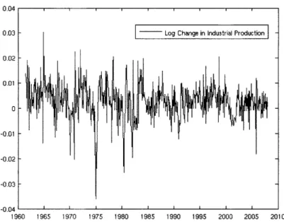
default .htm. An overall plot of the GIP over time is shown in Figure 3-1. The plot displays the log of the change in GIP over time sampled monthly. It can be seen that the volatility in the underlying data is extreme over time. In order to smooth some of these variations, an exponential moving average has been used with smoothing coefficient of p = 0.8221. The smoothed plot is also shown in Figure 3-2. In turn, the predicted one period ahead value of an ARMA(1,1) model is an exponentially-weighted moving average of past monthly values, with a decay coefficient equal to the moving average parameter. Further details on the smoothing were developed by Joslin et al. [14].
3.3
Proposed Tests and Results
The proposed tests deal with an alternate binning strategy to that used by Duffie et al. [4]. Figure 3-2 shows the smoothed GIP over time. The alternate binning strategy or GIP-based binning relies on creating bins based on sorting the exponentially smoothed log change in Industrial Production. This order then drives the order in which time intervals are considered for the binning strategy. This sort order would then allow one to measure statistics of default counts over varying levels of economic activity.
0.03 0.02 0.01 0.01 0.02 0.03 --0.04 I 1960 1965 1970 1975 1980 1985 1990 1995 2000 2005 2010
Figure 3-1: Log Change in Industrial Production
0.01
0.005
-0 005
-0.01
Smoothed Log Change in Industrial Production
-0,015
1960 1965 1970 1975 1980 1985 1990 1995 2000 2005 2010
Figure 3-2: Smoothed Log Change in Industrial Production
I-Table 3.1: Time-based Bins: Summary Statistics for Bin Size=8
Bin=8, Summary Statistics
Time Period Mean Std. Deviation Skewness Kurtosis 1985-1989 12.7778 5.2387 0.6865 2.5318 1989-1993 15.6667 9.8234 0.5658 2.2150
1993-1997 8.3333 4.1231 0.4174 2.6412
1997-2001 6.8889 5.7975 0.9584 3.0277
2001-2005 6.2222 5.6519 0.5857 2.4126
Table 3.2: GIP-based Bins: Summary Statistics for Bin Size=8
Bin=8, Summary Statistics
AGIP Quintile Mean Std. Deviation Skewness Kurtosis Quintile 1 10.4444 5.6372 0.8750 2.4866 Quintile 2 12.6667 8.2462 1.1835 3.7952 Quintile 3 9.5556 7.1783 0.2496 1.4846 Quintile 4 8.5556 6.6353 0.2035 1.9640 Quintile 5 8.3333 5.4544 0.2636 1.9635
This section details the results from tests devised by Duffie et al. using traditional time-based binning. Using data from 1985 through 2005 at three month intervals, time based binning yields results documented in Table 3.1 and Table 3.2.
As can be seen from Table 3.1, accumulated mean defaults are higher in the periods prior to 1994. This is in line with the relatively better fit for predictions seen in later periods. Although the number of defaults are higher, the extent of fit drives the accumulated mean defaults closer to the bin size of 8.
On the other hand, the Table 3.2 shows similar results from accumulated mean defaults when a GIP based strategy is used to measure defaults. This table shows that the standard deviations are higher during periods of lower economic activity and lower during periods of higher economic activity. In addition, the means are higher during periods of lower economic activity.
Chapter 4
Technical Architecture and Data
Overview
This chapter provides an in-depth view of the system and sub-system components as well as key elements of data analysis used to assemble firm default information. Several alternate sources of firm default information are available. The current work uses the COMPUSTAT Inactive firm database available through Wharton Research Data Services (WRDS). The choice of this data source was driven more by availability to a wide range of data in a time series format than any other factor. Other premium sources of this information include Moodys KMV and Bloomberg. Moodys KMV appears to be the premium source of default information. Data from Bloomberg was found to be available in a Point in Time snapshot as opposed to a Time Series. In addition, more data was available for recent dates than earlier dates.
4.1
COMPUSTAT Data Feed
This section presents an overview of the process used to obtain data from COMPU-STAT. This includes the queries along with the parameters and key data elements from the data sets.
4.1.1
The COMPUSTAT/CRSP Merged format
COMPUSTAT has a wide listing of inactive firms which include bankrupt and default firms. Although the current work is based on earlier work by Duffie, Saita and Wang [5], the data source used by that earlier work is being assimilated into the newer COMPUSTAT/CRSP merged database. The new merged format offers the same data elements organized in different sets of feeds. In addition, the earlier work used the
INDUSTRIAL format of the data on COMPUSTAT which, although available, is no
longer updated as of July 2007 (http: //wrds. wharton.upenn. edu/ds/comp/indq/). So the current work relies on the newer COMPUSTAT/CRSP Merged Fundamental Quarterly and Security Monthly databases.
The Fundamental Quarterly Feed
The Fundamental Quarterly feed provides both the firm meta information including security identifiers and Point in time firm data as well as the time series fundamental data required to compute the Distance to Default or other metrics required for the Reduced Form model. Both the Point in time information as well as the time series data rely on a common query specification which is described in the following section. The Fundamental Annual Query is identical to the Fundamental Quarterly table from a query perspective. Hence the following section is equally applicable to both feeds.
Basic Query Configuration The following parameters are used as part of the
Basic Query Configuration:
* The Date Variable is typically set to datadate.
* The Beginning and Ending dates are set to the minimum and maximum of the available range respectively
* Entire Database is chosen for the search method
* Consolidation Level set to default value of C
* Data Format set to STD. Add to Output can be unchecked.
* Population Source set to D for domestic. Add to Output can be unchecked.
* Quarter type set to both Fiscal View and Calendar View. This helps handle differences in end of quarter for firms which may not be aligned with calendar
date.
* Currency set to USD. Add to Output can be unchecked.
* Company Status set to both A and I for active and inactive firms
Security Meta Information and Point in Time data The Point in Time data
is derived from the Identifying Information and the Company Descriptor sections of the feed. Ticker Symbol, CUSIP and CIK Number are used in addition to all fields from the list beginning with the address lines. This list includes the DLRSN i.e. the delete reason and the DLDTE or the deletion date fields in addition to the GIC and S&P sector codes. These are critical to classifying the default events. Other useful descriptors include the AJEXQ or the Quarterly Adjustment Factor and the
APDEDATEQ or the actual period end date. The various delete reason codes are
interpreted as follows:
Reason code Reason for Deletion 01 Acquisition or merger 02 Bankruptcy
03 Liquidation
04 Reverse acquisition (1983 forward)
05 No longer fits original format (1978 forward) 06 Leveraged buy-out (1982 forward)
07 Other (no longer files with SEC among other possible reasons), but pricing continues
09 Now a private company
Security Time Series Data The Security Time Series information is largely
de-rived from the Quarterly Data Items and the Supplemental Data Items sections of the feed. Noteworthy fields in this section include the ATQ or Total Assets, LTQ or To-tal Liabilities, CSHOQ or Common Shares Outstanding, the ADJEX or Cumulative adjustment factor applicable to security returns.
Security Monthly Feed
Security Prices used in the model are derived from two possible alternate locations. Quarterly security prices are derived from the PRCCQ field in the Fundamental Quarterly table. However, Monthly security prices are derived from the Security Monthly Feed. All the Basic Query Configuration are applicable to the Security Monthly Feed. In addition, the Data Items are selected from the Variables section. Key variables from this section are AJEXM which is the Cumulative Adjustment Factor and PRCCM or the monthly Security Closing price. The Security Monthly feed provides data for both active and inactive firms.
4.1.2
Alternate Data Sources
Other core data items for the model were derived from two sources -Yahoo! Finance and Bloomberg. Yahoo! Finance provided the historical data required for 1 Year treasury bills, 3 Month treasury bills and historical closing prices for the Standard and Poors 500 Index. The GIC Sector definitions for the sectors, industries, groups and sub-industries were obtained from Bloomberg. The 1 year treasury bill rates are used to compute distance to default for all the firms in the underlying data set. On the other hand, short rates or the 3 month treasury bill rates are used as part of the core estimation set. The following definitions are applicable to the GIC entities:
* GIC Sector: Two digit code used to define high level Economic Sectors. Some examples include 10 for Energy and 25 for Consumer Discretionary
* GIC Group: Four digit code used to define sub groups within the sectors. Some
* GIC Industry: Six digit code used to define industries. Examples are 251020 for Automobiles, 252010 for Household Durables
* GIC Sub-industry: Eight digit code which represents the most granular classifi-cation of firms in this scheme. Examples include 15104030 for Gold or 15104050 for Steel.
4.2
Technical Architecture
This section provides an overview of the system components used in processing the data from COMPUSTAT and other sources to generate the state variables useful in the estimation process. In most cases, data from the COMPUSTAT and CRSP feeds are used without further modifications to create data model without any trans-formation. The estimation process, however, relies on data transformation from a security-time series format to a normalized security format described in more detail in subsequent sections.
4.2.1
System components
The sheer volume of data organized in a security-time series format prompts one to use a relational database format to store, use and update the data on a periodic basis. For example the current dataset, going as far back as 1960, consists of 26066 unique firms and 1,197.443 firm-quarters of data. This includes default as well as active firms. Each of the underlying firm-quarter entries consists of approximately 791 items which are various firm metrics and other items from the firm's quarterly balance sheet. Hence a relational database format lends itself well to the current model.
MATLAB is used as the platform for simulation and estimation needs. The data interfaces between MATLAB and the database are handled using the database toolbox in MATLAB. Beginning with an overview of the data architecture, this section also describes the key functions in MATLAB which can be used to perform various
sub-tasks in the modeling and estimation phase.
4.2.2
Database tables: Data from Finance Sources
Firm Quarterly Data The firm quarterly feed described earlier maps directly to the crspalLqdata table. In addition to the quarterly data items, this table also contains some basic security classification data, if such data flags were to be selected during the export phase, as described earlier. The composite primary key in this data table consists of the security identifier (or the gvkey in COMPUSTAT parlance) and the datadate which is the as-of date for the quarterly record. Additionally, indices have been created on the gvkey, datadate, tic and CUSIP fields for ease of use.
Firm Meta Information The firm meta feed maps directly to the crsp_all_qmeta table. This table contains all the firm specific data and identifiers provided at a quarterly frequency. Although there is significant redundancy in this data, it is not optimized as it provides a quick metric for how many data points exist per firm in the feed. Although the crsp_allqdata table could also provide this metric, the sheer size of the table makes it less efficient for such needs. This table provides the key delete reason code dlrsn which forms the basis of all further computation. Since this table also handles both inactive and active firms, a reason code of 0 is used for active firms. This table is also the source of the deletion date of dldte which is also the date the firm was recognized as deleted in COMPUSTAT. Often this is anywhere between 5-800 days after the security pricing is no longer obtainable. Hence the significance of this date in estimation or modeling use appears to be questionable.
Security Prices Security prices for both Active and Inactive firms are available at
different tables. For monthly prices, the PRCCM field in the crspsecprice table and for quarterly prices, the PRCCQ field in the crspalLqdata table is used. The feed for this table is directly sourced from the Security Monthly feed described earlier.
GIC Definitions Each of the underlying GIC definitions are stored in the four underlying tables: gic_ggroup, gic_gind, gicgsector, gic_gsubind. The definitions from each of these tables is used as a source for descriptive data for charts and plot legends.
Long and short treasury bill rates Historical data for long and short treasury
bill rates are stored in the yhoo_1yeartbill and the yhoo_3monthtbill tables respectively. The rates are quoted in percent and these two tables use the date of the record as the primary key. The treasury rates are available at a daily frequency but sampled at a monthly or a quarterly frequency depending on choice of time frame.
S&P 500 rates Historical closing prices of the S&P 500 Index, adjusted for
divi-dends and splits are present in the yhoo_sp500 table, indexed by date. The AdjClose field is used from this table to compute security returns which are used in further computation and also as one of the covariates in the estimation process. Although, this data is also available at a daily frequency, it is sampled quarterly or monthly depending on choice of time frame.
4.2.3
Database tables: Generated Data
The main difference between this section and the previous section is that data in these tables are derived from other tables or from other processes such as distance to default computation.
Input for estimation The input for estimation is organized into the est_input and
the est_input_stat tables and the est_input_maxdte view. The derived fields in each of the tables is covered below:
TABLE: est_input
* gvkey: The security identifier commonly used throughout COMPUSTAT
. dlrsn: Delete reason for firms which are inactive
* dldte: Deletion date of record for an inactive firm
* gsubind: GIC Sub-industry code which includes the Group, Sector, Industry and Sub-Industry codes. This is derived from the crsp_alLqmeta table
* dd: Distance to Default computed in MATLAB derived at a monthly or quar-terly frequency of choice.
* secret: Geometric Security Return derived from the security prices
* tbill3m: Three month treasury bill rate interpolated to be available at monthly frequency or directly derived at quarterly frequency.
* spret: S&P Geometric returns from the yhoosp500 table
* datadate: Date representation of the date of record
* defaultOccured: 0 for N periods before default occurs and 1 afterwards. This field is computed and set in MATLAB depending on choice of N in days.
* defaultCount: Number of firms which have defaulted in the last M months. This is computed and set via MATLAB. The last two fields are described in more detail in the following section dealing with the MATLAB modules.
TABLE: est_input_stat Unlike the estinput table, this table is normalized to one
entry per security. It is primarily used for normalized, grouped security data such as maximum market capitalization or other aggregate metrics. This table consists of the following fields:
* gvkey: COMPUSTAT security identifier
* maxcap: Maximum market capitalization for the security. This field is coin-puted and set via SQL
* maxtrd: Maximum trading volume per quarter for the security. This field is computed and set via SQL
* totcount: Total firm-quarter data points available for the firm. This field is computed and set via SQL. It is used to filter out firms which have less than N firm-quarters of data.
* selected: Flag which determines whether or not a firm is included in a given estimation input set.
* dlrsn: Delete reason
* dldte: Deletion date
* diffdtes: Difference in days between the deletion date and the actual date when security prices become unavailable
* gsubind: GIC sub-industry code
* maxdd: Maximum distance to default computed for the firm. This field is derived from the est_input table
* mindd: Minimum distance to default computed for the firm
TABLE: est_maxdte This database view contains the maximum date for which
security prices are available for the firm. As previously discussed, there is considerable difference between the deletion (late and this maximum date. For all further analyses and plots, this date is used as the maximum date in place of the deletion date. Since price availability drives the computation of metrics such as distance to default or security returns, lack of prices curtails the usefulness of other metrics.
4.2.4
Generating Estimation Inputs
The various steps involved in generating estimation inputs are listed below. These include discrete operations performed either in SQL or MATLAB to create a suitable input for estimation.
* Populate the tables listed under the Data from Finance Sources section. This table is populated one-time and does not need to be revisited unless there is a need to refresh the table.
* Run the process to estimate distance to default. The driver script assembleall.m drives this process. This process does not need to be executed more than once unless some of the core formulae or definitions for the fundamental covariates discussed in Chapter 3 change.
* Import the output of the estimation process into the est_input table. All fields except defaultOccurred and defaultCount are populated by the output from the estimation process.
* Populate the estinput_stat from the estinput table via SQL. The selected flag in this table is initially set to 0 for all firms.
* Execute the apply_selection function for firms with delete reason 0. Repeat the function for firms with delete reasons 2 and 3. Execute the update_default_occurred with a parameter in days for number of days prior to default event. Most of the examples in the current context use 180 for number of days prior to default. This script accounts for applying various filter criteria to the data such as max-imum market cap, average quarterly trading volume, days between maxmax-imum price availability and default date, minimum data availability, default reason codes, minimum and maximum distance to default.
Typical values applied to non-default firms are 0 (no market cap filters), 0 (no average trading volume filters), le10 (maximum difference between last price availability and default date. Since non-default firms have no defined default date, this value is typically large), 8 ( minimum quarters for which data is available), 0 (delete codes), -100 (minimum distance to default), 100 (distance to default), 0/1 (for insert / update mode).
Comparable values applicable to default firms are 0 (no maximum market cap-italization filters), 0 (no average trading volume filters) and 800 (maximum
difference between last price availability date and default date). Note on the default dates in COMPUSTAT
As previously noted, the default dates in COMPUSTAT are often late in indicating probable default. In many cases, these dates lag behind the end of price availability. The histogram below shows the variation in the lag with a mean lag of around 452 days with a variance of around 288 days. All offsets between 0 and 800 are used for this analysis. However, this is configurable, as previously discussed, and can be set by the apply_selection script.
700 600 [Mean= 452.45 Std = 288.38 500 400 8300 200 -100 -2000 -1500 -1000 -500 0 500 1000 1500 2000 2500
Days between Deletion Date and Max data avail
Figure 4-1: Distribution of Days between End of Price and Default Date
Also shown below is a summary view of the defaults across four different sectors which has been extracted from the COMPUSTAT data source. In this plot, the Economic Sector definitions are derived from the standard GIC sector definitions. As can be observed from the plot, defaults are higher across the Consumer Discretionary and the Information Technology sectors. On the other end of the spectrum, Energy and Utilities, by definition being more stable than other sectors have lower levels of default. This also leads one to the observation that the inherent default intensities in these underlying sectors can be expected to be different. Chapter 5 discusses sector
40 . 30 10 0 1975 1980
Economic Sector: Utilities Economic Sector: Energy
Economic Sector: Information Technology
Economic Sector: Consumer Discretionary
Figure 4-2: Actual observed defaults in various sectors between 1980 to 2004
specific estimation of default intensities in line with these sector definitions.
44
I I ;
25 4 20)05 1 23
Chapter 5
Model Extensions and Results
5.1
Introduction
As previously discussed in Chapter 3 and Chapter 4, the base model presented by Duffie et al. discussed a doubly stochastic model of firm default intensities across various default types, consisting of both a historical and a predictive component. The data overview in Chapter 4 reviews the default events in COMPUSTAT which are studied in the current context. In addition, it can be postulated that the model parameters are different for the various sectors not only due to inherent differences in how the firms are managed but also because of how sensitive the firms are to changing macro-economic conditions. Although the dataset used in the current exercise is derived from COMPUSTAT, it differs from that used by Duffie et al. as the default events have not been augmented using Moodys or other sources. Hence, the model parameters can also be expected to be different.
Using the doubly stochastic assumption, this chapter describes the derivation of model parameters and explores alternative model covariates which could potentially improve the overall model fit and predictive ability. Calibration of this model is performed using search based on Constrained Minimization. This is discussed in the next section followed by key results, plots and interpretations.
5.2
Model Calibration
Chapter 4 describes the source of the default data and various types of failure events such as Bankruptcies, Defaults, Liquidation etc. In order to calibrate the model, the following structure, also derived from the Duffie et al. work [5] has been used for the default intensities:
A(X) = eP =1 x (5.1)
This results in a double exponent expression for the default probability which is defined as
Default Probability (p) = 1 - e- A*t (5.2)
The advantage of this structure for the default intensity is that it ensures a positive value for all values of the covariates. However, there is some additional potential for the expression to be more sensitive to changes in underlying variables compared with a more traditional CIR form of the expression. With the above definitions, the probabilities of the default events can be maximized using a log likelihood function. Clearly, this constitutes a non-linear problem which can be maximized using most commercial solvers.
5.2.1
Econometric Background for Model Calibration
The default intensity of a borrower is the conditional mean arrival rate of default, measured in events per unit time. Duffie et al. [5] showed that, if (M,N) is a doubly-stochastic two-dimensional counting process driven by X, then intensities can be defined as:
a = {at = A(Xt) : t E [0, oo)} for M (5.3)
A = {At = A(Xt) : t >= 0} for N (5.4)
This also implies that, conditional on the path of X, the counting processes M and N are independent Poisson processes with intensities a and A. In this framework, it is important to recognize that a given firm exits and ceases to exist when the earlier
of the two events, M or N occur. Also the state vector Xt ceases to be observable when the firm exits due to one of the two events. Duffie et al. also show the following
two results:
P(T > t + s Ft)= p(Xt, s)= E(eft" -(A(u)+a(u))du Xt) (5.5)
P(T < t + sIF) = q(X, s) = f E( + e-(()+(u))dui(z)dz|X,) t (5.6)
Likewise, it has also been shown that a maximum likelihood function which max-imizes the probability of the exit events given by the above expressions can be cast into the form below for events of type p.
sup,,
fle
fi° A(X';")dU(lHirT + A(X(T); p)1H=Tr) (5.7)i=1
Similarly, the likelihood function for another type of exit event v is
sup, f3 e-
£I
A(Xu;v)du(lHi T + A(Xi(T); V)1Hi=Ti) (5.8)i=1
Duffie et al. also show that the likelihood functions expressed above can be de-composed into a pair of problems. Solutions to the problems above form a solution to a parameter vector 03 taken in a decoupled form with parameters ,P and v.
In the current context, A is defined as the default intensity of the process which drives the firm into default in the next six months. This is done in order to avoid any boundary effects from improper security returns when the firm is close to default or when the security prices for the firm become unavailable due to delisting or other market events.
5.2.2
Constrained Minimization to Optimize the Likelihood
Constrained minimization can be used to optimize the negative of the log likelihood defined by 5.7 and 5.8. This technique relies on a gradient search of the optimization
space in order to minimize the objective function. The first order optimality in this context is derived from work developed by Karush, Kuhn and Tucker (KKT). This approach is analogous to that used in regular gradient search modified to incorporate constraints.
The KKT technique implemented in a solver such as MATLAB also allows for various thresholds to optimize the overall solution time. Thresholds can be specified on size of the search step, delta of the objective function, maximum tolerance on the number of constraints violated as well as heuristic limits such as maximum number of function evaluations. In addition specific variables can be fixed while letting others vary for greater flexibility.
5.3
Results and Interpretations
5.3.1
Reduced Form model for Default Intensities
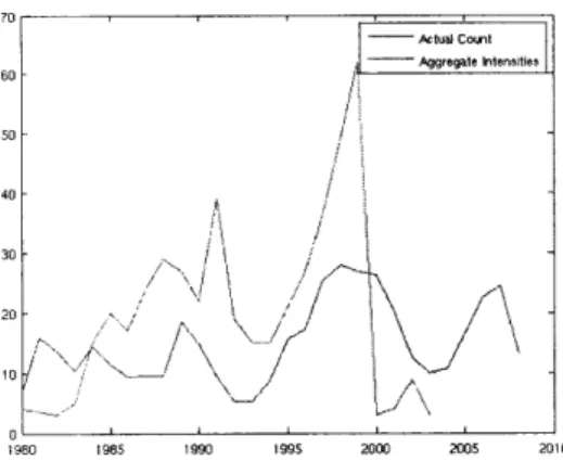
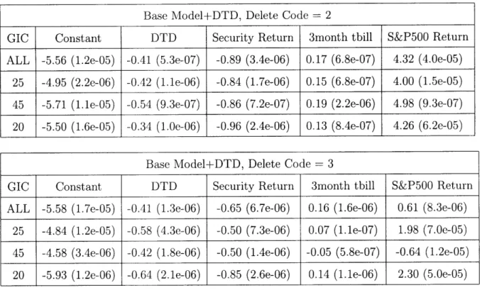
Several alternate model structures are examined below with varying degrees of fit to observed default counts. In addition, tests prescribed by Duffie, Das et al. [4] have also been carried out to test the doubly stochastic assumption. In order to examine the impact of Structural Parameters such as Distance to Default, the base model is defined to be one with only three basic covariates - one firm-specific covariate, the one year trailing Security Return and two global covariates, the Three Month T-Bill and the one year trailing S&P500 Return. In addition, plots of key parameters such as Firm Default Intensities or Aggregate Market Default Intensities are also shown in order to assess model fit.
Sample Plot: Firm-Specific Default Intensities
The plots in this section show the firm specific default intensities as a function of time for a handful of firms which exited through default code 2 or default code 3 in COMPUSTAT. The model structure discussed by Duffie, Saita, Wang [5] was used in producing these plots. In most of these cases, it can be seen that the default