HAL Id: hal-00687277
https://hal.archives-ouvertes.fr/hal-00687277
Submitted on 13 Apr 2012HAL is a multi-disciplinary open access archive for the deposit and dissemination of sci-entific research documents, whether they are pub-lished or not. The documents may come from teaching and research institutions in France or abroad, or from public or private research centers.
L’archive ouverte pluridisciplinaire HAL, est destinée au dépôt et à la diffusion de documents scientifiques de niveau recherche, publiés ou non, émanant des établissements d’enseignement et de recherche français ou étrangers, des laboratoires publics ou privés.
Intra-Household Inequality in Transitional Russia
Ekaterina Kalugina, Natalia Radtchenko, Catherine Sofer
To cite this version:
Ekaterina Kalugina, Natalia Radtchenko, Catherine Sofer. Intra-Household Inequality in Transitional Russia. Review of Economics of the Household, Springer Verlag, 2009, 7 (4), pp.447-471. �hal-00687277�
Intra-Household Inequality in Transitional Russia
Ekaterina Kalugina Natalia Radtchenko
Catherine Sofer
June, 2009
The paper proposes an original strategy to analyze household sharing of income and satisfaction. Using two different subjective questions of the Russian data RLMS (Russia Longitudinal Monitoring Survey), we assume a correspondence between, first, the perception of income that household members report and their true income sharing, and, second, between their answer to a satisfaction question and their utility. We show that the answers given by different members of the household bring pertinent information on income sharing and utility in the household. In particular, we find a significant effect of the female-male wage ratio in reported income perception and satisfaction differentials between household members. Given that the available data covers the transition period (1994-2003) characterized by massive economic and social changes in Russia, we investigate the dynamics of household behavior.
Keywords: subjective data, intra-household inequalities, transitional Russia JEL Classification: D13, I31, C3, P36.
1. INTRODUCTION
The objective of this paper is to show that subjective data can be used to test directly some of the assumptions made in non-unitary models of the household. Non-unitary models share a common view of decision-making within the household, where final allocations, i.e. consumption and labor supply of household members, depend on their “bargaining power”. This is true whether the decision-making process can be represented by a cooperative game (Manser and Brown, 1980; McElroy and Horney, 1981; Lundberg and Pollak, 1996), by a non cooperative game (Bergström, 1997; Chen and Woolley, 2001; Konrad and Lommerud, 1995 and 2000; Lundberg et al., 1997; Udry, 1996; Ulph, 2006), or is only assumed to be Pareto-optimal, as in collective models (Bourguignon and Chiappori, 1992; Browning and Chiappori, 1998; Chiappori, 1988 and 1992; Moreau and Donni, 2002).
Starting with non–unitary approach, we introduce two concepts defining intra-household equality. Our strategy consists in using subjective data to infer intra-household sharing of income and satisfaction and applying probit-type model accounting for discrete unobserved heterogeneity. The empirical findings refute the unitary model hypothesis regarding income pooling at the household level and support the assumptions made by bargaining models. In particular, we show that relative wages and age difference of spouses impact the sharing of income and utility1.
The intra household welfare distribution is analyzed in its dynamics during the transitional period in Russia. The economic transition from a centrally planned system to a market economy introduced since 1992 led to dramatic changes in the Russian economy and was accompanied by a considerable fall in individual and household incomes (Mikhalev, 1998). According to official data (Goskomstat, 2000), during the period 1991 -1999, the GDP decreased by 37% and industrial output fell by 54%. The country suffered from high and continuing inflation. By mid 1998, the Russian economy was showing signs of recovery, but in August 1998 the country faced a severe financial crisis accompanied by a devaluation of the ruble, default on both domestic and foreign debts, and a collapse of the stock market (Lokshin and Ravallion, 2000). For many Russians this crisis was reflected in a considerable real wage decline: -13.3% in 1998 and -22% in 1999 (Goskomstat, 2004). Since 1999, macroeconomic indicators look better: continuous GDP growth starting in 1999 and growth in real wages and employment (Goskomstat, 2008).
1 Our findings are also consistent with Becker’s theory of marriage (1981) according to which a woman’s
The economic crisis seriously impacted the labor market: according to RLMS data, the wage gap between men and women increased significantly during and after the crisis (Gerry et al., 20042; Glinskaya and Mroz, 2000; Lacroix and Radtchenko, 2008). Men often moonlighted while women increased their domestic labor supply. These behavioral changes can not only have distributive impacts within households but they can also induce changes in social norms, more specifically a movement away from the emphasis on equal employment of men and women during the communist period3. In recent years, a significant proportion of women have withdrawn from the working force to become housewives while at the same time young women have become more active, more inclined to embrace professional careers and more mobile in labor markets.
All these trends inevitably influence intra-household relations and consequently the decision process.
The next section presents the data and discusses some Russian labor market adjustments. Section 3 presents the descriptive statistics of subjective questions and validates the assumptions regarding subjective data. Section 4 introduces two concepts defining intra-household equality and consequent econometric applications. Section 5 discusses the main empirical results. Section 6 concludes
2. LABOR MARKET ADJUSTMENTS IN RUSSIA: DATA AND
SOME STYLIZED FACTS
The data come from the Russian Longitudinal Monitoring Survey (RLMS), a database jointly collected by UNC Chapel Hill (USA), the Russian Academy of Sciences, and the Russian Institute of Nutrition. The RLMS is a household–based representative survey designed to measure the effects of the reforms implemented through the 1990s on the economic well-being of households and individuals. The survey has two phases: during the first phase of the project (1992-1994), the RLMS collected four rounds (I – IV) of data on 5900 households on average; since 1994 the RLMS has collected eleven further rounds (V -
2
Gerry et al., (2004) provide evidence that the wage gap is unevenly distributed, with women at the lower end of the distribution suffering most. Their results show that managers very likely used wage arrears and in-kind payments to attenuate the wage gap at the bottom end of the wage distribution
3 However, society remained predominantly patriarchal and gender relations within the household continued to
XV) of data in the second phase of the project. The second phase data were drawn anew from the population and contains approximately 4000 households4.
We use first eight rounds of phase II (rounds 5 – 12). Our analysis covers the period from 1994 to 2003, a period characterized by massive economic and social changes in Russia.We follow Lacroix and Radtchenko (2008) in considering two major sub–periods of the phase II corresponding to the pre and post financial crisis periods characterized by different economic trends.
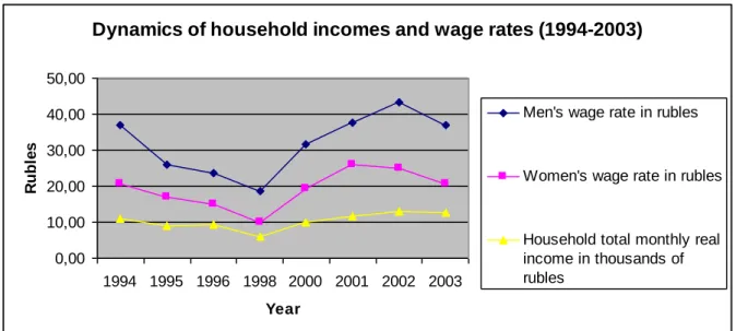
Figure 1 shows mean values for real wage rates (in 2003 rubles separately for men and women) and household income for working couples (in thousands of rubles). When measuring the wages5, we account for such phenomena as moonlighting and the development of informal activities (Foley, 1997; Schneider and Enste, 2000) using the information provided by RLMS about the individual’s job (primary, secondary or informal activities). Moreover, we account for public / private type of working place for primary and secondary jobs: the corresponding question is the following: « Is the government the owner or co-owner of your enterprise or organization? ». According to our data, starting with 68% of working individuals working in firms where the government is the owner or co-owner in 1994, this share diminished to 52% in 2003. The distinction between the private and public sectors is important as the public sector offers low wages (Gimpelson and Lukyanova, 2006), but, in return, provides greater job security and numerous benefits which are generally not offered by the private sector (Yemtsov et al., 2006).
Trends in household total monthly income and wages globally correspond to the Russian economic situation of the period. Household total monthly real income declined between 1994 and 1995, slightly increased in 1996, then considerably decreased in 1998. The trend is positive between 2000 and 2003, with a slight decrease in 2003. We observe thus the impact of the financial crisis of 1998 and the subsequent recovery starting 2000.
4 All necessary information on the RLMS data could be found on the data web site:
http://www.cpc.unc.edu/projects/rlms. Only first 13 rounds are available free of charge
5 Russia’s transformation into a market economy has given rise to the emergence of specific labor market
phenomena such as wage arrears, payment in-kind, compulsory unpaid leave, reduced working hours etc. (Gerry et al, 2004). Such non-standard labor market institutions as well as an underreporting or non responding of monetary indicators in the data are likely to affect the wage measurement. However, these difficulties were especially acute at the beginning of the transition period and, after 2000, the situation has been improving considerably. By considering the pre and post financial crisis sub-periods, we account for such phenomena in our empirical strategy.
Figure 1. Dynamics of household incomes and wage rates (1994 – 2003)
Dynamics of household incomes and wage rates (1994-2003)
0,00 10,00 20,00 30,00 40,00 50,00 1994 1995 1996 1998 2000 2001 2002 2003 Year R ub le s
Men's wage rate in rubles
Women's wage rate in rubles
Household total monthly real income in thousands of rubles
Source: RLMS (round 5-12), working couples.
Radtchenko (2006) and Lacroix and Radtchenko (2008) investigated the evolving Russian labor market adjustments for the same period. They show that wives’ wage rates have decreased significantly relative to husbands’, starting with the financial crisis of 1998. Nevertheless, their participation rates and their workweek have remained relatively stable, leading to a decrease in wives’ share of household income over that period. The adaptation to the major economic downturn of 1994-1998 and to the eventual recovery of 2000-2004 have brought spouses to a new economic equilibrium and consequently have impacted the intra-household distribution of welfare within Russian intra-households.
3. USING SUBJECTIVE DATA
3.1 Subjective well-being: some descriptive statistics
Following the work on poverty initiated by the « Leyden School » in the seventies, subjective data are more and more extensively used in the economic literature, especially in studies about poverty, well-being, satisfaction, or happiness (Ferrer-i-Carbonell and Frijters, 2004). Many national surveys, such as the British Household Panel Survey (BHPS), the
German Socio-Economic Panel (GSOEP) or the RLMS, ask questions about satisfaction in
these questions most often take discrete values ranging which are generally used as proxies for individual well-being (Senik, 2005).
Reliability and validity of peoples' answers have been extensively studied in the recent literature. Easterlin (2001) has pointed out that "the general conclusion of such assessments is
that subjective indicators,…, though not perfect, do reflect respondents' substantive feelings of well-being" (also see Diener, 1984; Diener et al., 1999; Veenhoven, 1993). For example,
subjective information is used to study individual non monetary costs of unemployment (Clark and Oswald, 1994; Winkelmann and Winkelmann, 1998) or to better understand individual attitudes towards inequalities (Ng, 1996; Ravallion and Lokshin, 2000). This kind of analysis generally provides plausible and reliable empirical results.
Each year the RLMS investigates the distribution of welfare in a qualitative manner. Spouses are asked to answer the Income Perception Question (1) and General Satisfaction Question (2):
1) “Please imagine a 9-step ladder where on the bottom, the first step, stand the
poorest people, and on the highest step, the ninth, stand the rich. On which step are you today?"
2) “To what extent are you satisfied with your life in general at the present time?” The possible answers are: “fully satisfied”, “rather satisfied”, “both yes and no”, “less than
satisfied”, “not at all satisfied”.
Our sample is composed of couples in which individuals gave answers to the above questions and provided wage information. To present self-rated income, we collapse the highest ranks (6, 7, 8, and 9) of the ladder into one category: few respondents considered themselves as amongst the richest.
Table 1 summarizes the distribution of self-rated economic welfare. We can observe the dynamics of the number of individuals feeling poor during the analyzed period: if we take the lowest two rungs to be the subjectively poor, the subjective poverty rate rose from 20.16% in 1994 to 24.69% in 1998 and then fell to 12.08% in 2003.
PLACE TABLE 1 HERE
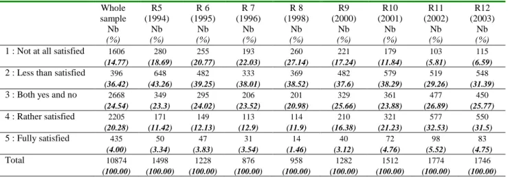
Descriptive statistics on general satisfaction are presented in Table 2. It is striking to see the level of non-satisfaction during the years 1994-1998, when Russia experienced a deep economic crisis. The situation is more positive during the four years after the crisis. 2002 is the best year in terms of satisfaction in our data. However, in 2003, we still have
approximately 40% of the sample unsatisfied and only 5% of respondents report that they are fully satisfied. These answers are very different from those obtained to the same question in Western Europe, where a large majority of people report being satisfied (Blanchflower 2001; Blanchflower and Rauner, 2006; Clark and Maurel, 2001).
PLACE TABLE 2 HERE
Table 3 presents differentials in the income perception responses of men and women. We consider answers of household heads, and compare their answers to those of their spouses6. In more than half of the households, men and women give different answers to the subjective question. Approximately 18% of men felt one step poorer than their wives and 8-10% of them differed by more than 2 steps. On average, women reported lower self-reported incomes than men in the same households, with the exception of the first year of observation (1994). For example, in 1998, the wives reported lower self-reported income in over 35% of households, while husbands reported being poorer than their wives in only 28% of households. However, in 2003, this difference was only 2% (32.02% versus 29.94%). This is not surprising if income sharing is the result of a bargaining process. Therefore, income is not necessarily shared equally by husbands and wives.
PLACE TABLE 3 HERE
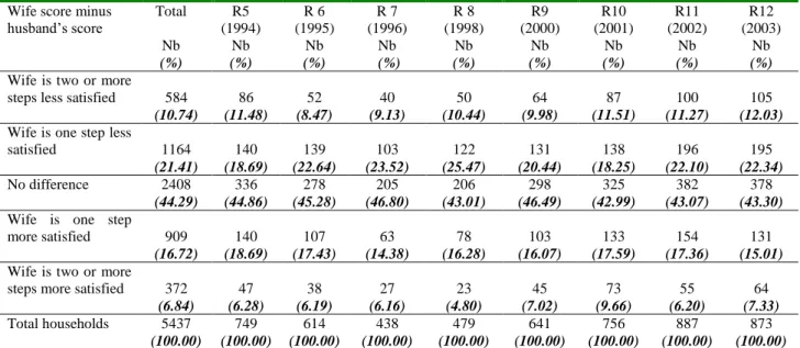
The descriptive statistics of within-household differentials in the responses to the satisfaction question are presented in Table 4. In more than 50% of households the answers are different. The number of husbands declaring higher satisfaction than their wives is higher than vice-versa. This difference is clearer than in case of self-rated income. The most “equal” year is 2001 (29.76% of households where wives are less satisfied versus 27.25% of the households where the opposite is the case). In 2003 there are 34.37% of the households where wives are less satisfied than their husbands while there are only 22.34% of the households where men are less satisfied.
PLACE TABLE 4 HERE
6 We consider all couples in the sample, married or not. The household head is defined as a male between 18 and
60. If no males in household, then the household head is a female between 18 and 55. If no middle-ages in household, then youngest elderly male (or female if male doesn’t exist) is considered to be the household head. Finally if none exist, then the oldest young person is the household head.
The answers of husbands and wives to both the questions relative to income perception and to utility show a similar pattern. Overall, the descriptive statistics suggests that their differentials can be associated with intra-household inequality, thus providing information on true welfare sharing in the households.
It also suggests that spouses have had to adapt their behavior to a changing economic environment. The behavioral adjustments may reflect not only gender-biased crisis effects, but also a new equilibrium bargaining power within households. Thus, we consider two different periods of time when using the data. To do this, we introduce a dummy variable D which takes a value of 1 for the observations of the post-crisis period (2000-2003) and a value of 0 for the pre-crisis period (1994-1998). In order to allow the parameters to vary with time, we complete the list of explanatory variables by their products with the dummy D. Thus we introduce two sets of explanatory variables for the empirical analysis throughout the paper: the coefficients corresponding to one set (D = 0) report the effects in the pre-crisis period; the coefficients corresponding to their products with the dummy provide the markup or markdown with time (D = 1).
3.2 Interpreting Answers to the Subjective Questions
We assume throughout the paper that differentials in the answers reflect differentials in the “objective” situation of household members.
First, we assume a direct relationship between the partners’ subjective answers and the income they objectively receive within the family on one hand and with their satisfaction level, on the other hand. We interpret a similar answer of the partners as indicating an equal sharing of income in the first case, and of utility in the second case.
Second, our interpretation of the available subjective information implies that the answer to the income perception question refers to household income sharing rather than to individual earned income.
Finally, our approach implies the comparability of the answers of different people: people live in different social environments, thus their answers about welfare or about income would merely reflect their individual position relative to their own social environment. An individual’s reference group for earnings, could be his/her work colleagues, or the group of people of the same age and educational level. If husband and wife did not have the same reference group, comparing their answers would not be meaningful. However, it makes sense
to assume that two individuals living together and sharing the same social environment have similar scales when answering subjective questions regarding economic well-being.
Two empirical tests given in the next subsections support our understanding of the nature of the information provided by the subjective questions presented above.
Income or Utility?
We estimate an ordered probit in order to test for a positive relationship between individual indirect utility, as measured by the answers to the satisfaction question (AS, the five steps satisfaction scale), and full income, as measured by the answers to the income question (AI, the nine steps income scale). While a positive relationship does not give a formal proof of the interpretation of AI as representing the shares of full income, it supports such an assumption and gives a direct test of the consistency of the answers to the two subjective questions.
PLACE TABLE 5 HERE
Table 5 shows a strong positive relationship between the answers to the income perception and satisfaction questions. Such a result is consistent with the theoretical interpretation (see below section 4): indirect utility function being increasing in income as well as in full income, a positive correlation between the two questions is expected when controlling for demographic variables. Note that the satisfaction scale is also increasing in wages. What can also be noted is the negative sign of children on their parents’ satisfaction. This is true for older children (7-18 years) upon their father’s satisfaction, and for children of any age upon their mother’s satisfaction. These latter strong negative effects are possibly related to the burden of total work (domestic work plus market work), which is very high and shared in a very unequal way (in Russia the total amount of work performed by women is much higher than amount of work performed by their partners, cf. Kalugina, Radtchenko and Sofer, 2008). As young children add much more work to their mother than to their father, it is not surprising that woman’s satisfaction decreases more with the presence of a young child.
Individual or Household Income?
The income question is asked on an individual basis within the individual questionnaire and does not explicitly refer to household income-sharing. However it is placed
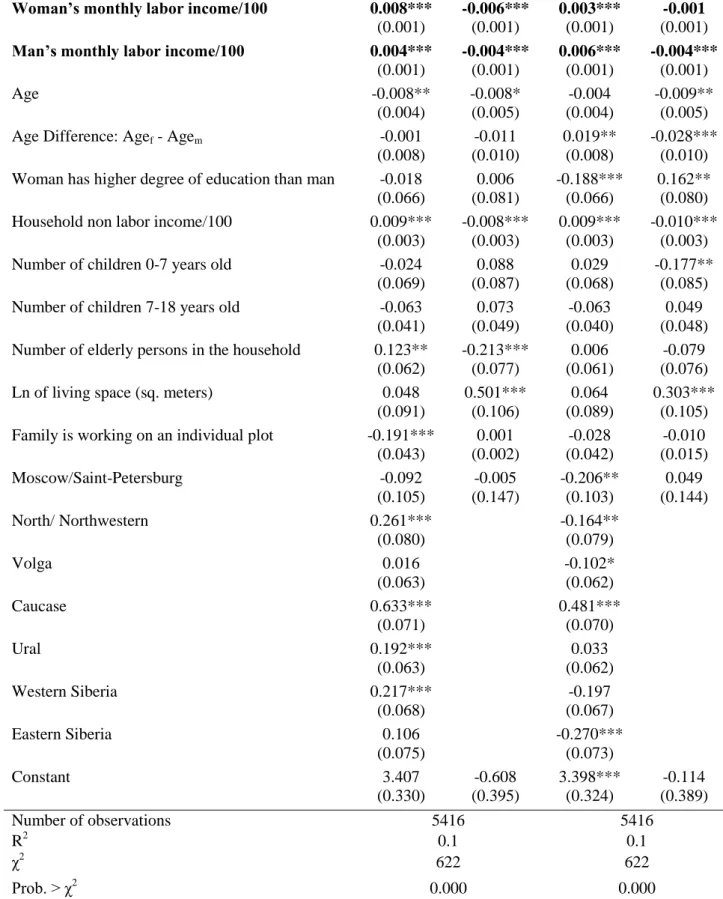
in the family well-being context. We assume thus that when answering this question, individuals refer to their share of household full income rather than to their individual labor earnings. To validate this assumption we carry out an empirical test which consists in regressing simultaneously the spouses’ values of income index AI on their labor incomes along with some individual and household characteristics. The results of the test are obtained using 3SLS and shown in Table 6. For each spouse, 0 gives the parameter estimate for the before-crisis period, 1 shows how it changes with time; the parameter corresponding to the post-crisis period is thus sum of 0 and 1.
PLACE TABLE 6 HERE
The data support our assumption. Indeed, if one’s reply referred to purely individual labor income, the partner’s labor income would not be significant. Both responses are strongly influenced not only by one’s own income, but also by one’s partner labor income. In general, for both spouses, the impact of one’s own income is greater than that of his/her partner income. These findings are consistent with non-unitary approach (see, for example, Bourguignon and Chiappori, 1992) and support our interpretation in terms of income sharing. Indeed, while one’s income increase can be benefic to both partners, the one’s increasing bargaining power due to increasing of his or her wage benefits stronger one’s own income share.
In addition, the test provides a first piece of evidence on the parameter changes between two periods. Indeed, the parameters corresponding to the income effects are in general varying with time: in difference with the pre crisis period, the income effects of both spouses become the same regarding the man’s response and the husband’s income does not seem to affect the wife’s response. This finding is very similar to that found by Lacroix and Radtchenko (2008): using a collective model of labor supply, they find that in this period, an increase in male wage translates in a smaller transfer to their spouse while an increase in female wage translates in a greater transfer to the husband. These changes are observed when controlling for differences in age and education of the spouses as well as in household composition and region of living.
4. MODELLING INTRA-HOUSEHOLD INEQUALITIES
The distribution of welfare within households is not egalitarian. The results of Sections 2 and 3 lead to the one of the basic hypothesis of the non-unitary models: each household member is doted by his or her own utility function. The indirect utility function depends on wage and individual full income, i.e. the sum of monetary and non monetary income. The allocations of the individual shares result from some negotiation process within the households.
Based on this hypothesis we define intra-household equality in two ways:
1/ as an equal distribution of the full income, i.e. of the sum of monetary and non monetary income:
m f
where f and mrepresent the wife’s and the husband’s full income amount, respectively. These amounts are a function of variables such as prices (here wages) or individual characteristics.
2/ as an equal distribution of well-being measured by his/her utility level V:
f f
f w
V , =Vmwm,m
where wf and wm are the wife’s and the husband’s wage respectively.
Given the available subjective information we construct two indexes of within household equality in order to analyze empirically intra-household inequalities.
Let IR and IS be indexes taking values 0, 1, or 2, depending on whether the difference observed between female and male income or satisfaction levels is negative, zero, or positive.
Intra household equality is formalized as follows:
0, if f m IR= 1, if f m
(1)
2, if f m 0, if Vf
wf,f
Vm
wm,m
IS= 1, if Vf
wf,f
Vm
wm,m
(2)
2, if Vf
wf,f
Vm
wm,m
Models (1) and (2) are estimated using an ordered probit model.
Let t indicate the year and D index the parameters before (D 0) and after the 1998 crisis (D 1). Let0, 1and Dreflect changes in the parameters so thatD 0 1D. Let
it
Z be the vector of individual characteristics of household i that proxies household preferences that may affect intra household welfare distribution. Furthermore, letit and i represent unobserved heterogeneity variables that are time-dependent and time-independent respectively. The latent variable g* associated with models (1) or (2) then represents differences in income shares (f m), in the case of IR, or in utility levels (Vf Vm), in the case of IS:
j it it D it g* γ Z
The contemporaneous error term it is supposed to follow a standard normal distribution and assumed to be independent of the random effectj
. Following Hoynes (1996), we assume that the individual random effect follows a discrete distribution with a finite number of realizations7. We thus assume, that the term j
occurs with probability j
P ,
J
j 1,..., , where J denotes number of possible types of households.
The model is estimated with only two types of households, as the data do not support further parametrization. The corresponding likelihood function is given by:
0 : 2 1 1 I i j j it D j P k F L γ Z
1 : 2 1 1 2 I i j j it D j j it D j P k F P k F γ Z γ Z
2 : 2 1 2 1 I i j j it D j P k F γ Z , 7Such a method allows not to constraint the random effect to follow a particular distribution law. The method is adopted in recent literature on household well being: Michaud and Vermeulen (2006) have recently estimated a discrete-choice collective household labour supply model in which unobserved heterogeneity is modelled in a similar fashion. Lacroix and Radtchenko (2008) have estimated in the same spirit a collective model with corner solutions using the RLMS data.
with F standing for the cumulative standard normal distribution function and two types of auxiliary parameters defining the latent variable bounds for each type of households:
1 1 1 k k k21 k2 1 2 1 k k k22
k25. RESULTS
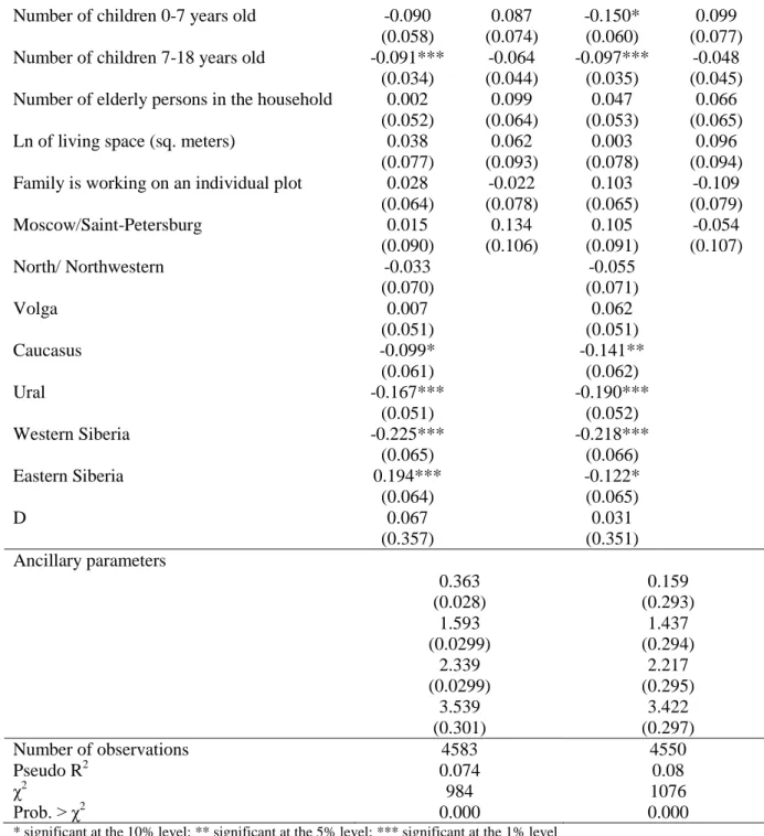
The parameter estimates of models (1) and (2) are presented in Table 7. For each index, the parameter estimates are divided into two columns, depending on whether D 0 or
1
D : 0 gives the parameter estimate for the pre-crisis period and 1 shows how it changes
with time; the parameter corresponding to the post-crisis period is thus the sum of 0 and 1.
PLACE TABLE 7 HERE
Table 7 shows that, for both indexes, wage difference is highly significant. First, this finding supports our hypothesis of a comparability of the answers discussed previously: indeed, if the appreciation scales of two partners were unrelated, the differentials in answers would not be dependent on wages or on the wage ratio.
Second, the coefficients corresponding to the wage difference has the expected sign: the higher the woman's wage compared to her husband’s, the greater is the probability that the woman's response to the income perception question is higher than her husband’s. Wage differences affect satisfaction differentials in the same way. However, the effect is less important for satisfaction than in the case of income. This is not surprising for it can be expected that wages have a stronger impact on income perception than on life satisfaction which also depends on many other variables, such as health, or family relationships. The two different indexes (IS against IR) are of a different nature. Indeed, these findings along with the positive correlation found between individual reported levels in income perception and satisfaction (Table 7) support the hypothesis of a relationship, but not of equivalence, of the two questions. For example, differences in expectations or in “needs” between the two partners will be reflected in the answers to the satisfaction question, more than in the answers to the income perception question. Conversely, the impact of the market determinants is expected to be much lower in the answers to the former than in the answers to the latter.
The monetary nature of the subjective income information is confirmed further by time flexibility of the differentials between the pre and the post 1998 periods. According to Table 7, the effect of the wage ratio decreased in the post 1998 period while its effect on satisfaction remained relatively stable. The effect of the wage ratio on income perception differentials remains nevertheless significant. The latter result could indicate that given a wage gap, the sharing of monetary resources is probably more equal in after crisis period.
As discussed previously, labor income during transition varied not only with the wage rate but also with the social security system accessible according to state or private status of an enterprise. Then, not only differences in wages but also differences in the job status could affect their satisfaction levels. The dummy variable “Working State Enterprise” indicates whether both spouses work in a state enterprise or not8. The negative coefficient of the post-1998 period in the IS estimation shows that women are less satisfied than men when work in a state enterprise in the post-1998 period. This could indicate the lower level of the social security system provided by state enterprises in the post-1998 period9, which is likely not to compensate any more for the low wages they offer. Indeed, the supply of public goods by state firms tended to decline after 1998, including facilities for children10.
Another variable which influences the distribution of full income and utility among household members is the age difference, i.e. the wife's age minus her husband's age: the older the woman relative to her husband, when the man’s age is controlled for, the lower her relative income and satisfaction perception. The effect of the age difference can thus be interpreted as showing the greater bargaining power of women who are relatively younger compared to their husband, all other things being equal.
Labor market liberalization was expected to lead to an increase in the returns to schooling over the transition period. Several studies (for the review cf. Flabbi et al, 2007) suggest that the largest increase in returns to education took place during the early transition (around the early 1990s) with returns to schooling higher for women than for men (Fleisher et al., 2004). Our results show that women having a higher degree of education than men11 used
8 In our estimation sample we have 47% of households where two spouses work in the firm owned or co-owned
by the government. This share has been decreasing during the analyzed period from 54% of such households in 1994 to 39% in 2003.
9 The detailed analysis of monetary and non monetary benefits proposed by the private and public sectors is
given in Radtchenko (2006).
10 According to our data the sharp decline of some social benefits within firms (free treatment in a department
medical institute, free or partial payment of sanatoria, free childcare in a departmental preschool) was observed between 2002 and 2003. The trend is true for both public and private enterprises.
11 Newell, Reilly (1997) and Gerry et al. (2004) show the advantages of using a set of educational qualification
in place of years of education in transitional economies. We follow the same approach when introducing education differences.
to gain in intra-household income distribution in the pre 1998 period. This positive effect cancels after the crisis. On the other hand, conversely, the after crisis period shows a positive effect of women’s higher educational level on satisfaction differential. As a whole, the results seem to indicate that an increase in the educational level relative to one’s partner increases one’s negotiation power. The same result is obtained in Kalugina, Radtchenko, Sofer (2009). A significant effect of age and education differences was also found in Bonke and Browning, 2003. (see also Grossbard-Shechtman, 1993 and 2003 on the effect of relative income and youth regarding woman’s access to household income).
Young children under seven exert a strong negative impact on differential in satisfaction in the pre 1998 period. In the post 1998 period the effect is positive on income distribution but remains negative on utility distribution. The positive change can be due to the relative economic growth observed after 1998. On the other hand, the negative effect on satisfaction differential is likely to indicate an unequal sharing of total labor between the partners (including household work) related to the presence of very young children. Indeed, Kalugina et al. (2009) find a negative effect of pre-scholars on women’s share of the household income when the former includes her leisure time evaluated at the market opportunity cost.
It should be noted that families with small children (under 18) are the most vulnerable population in terms of poverty in Russia (Ovcharova, 2005)12. However, the result of this negative influence of the number of children on life satisfaction could also be found for other countries. For example, Clark and Maurel (2001) using the RLMS for Russia and BHPS for Great Britain found that in both countries life satisfaction is significantly lower for households with more children. Alesina et al. (2004) also find a negative effect of children for 13 countries (12 European countries and the USA) interpreting this as “children seem to bring
about preoccupations, stress and hard work”. Let us stress here that what we find is that
(young) children affect differently their mother’s and their father’s satisfaction.
The presence of elderly persons decreases the woman’s share of household income in the post 1998 period. Though, a positive impact was found in a pre crisis period. This result has no easy interpretation. It could mean that women are likely in charge of financing (on their “budget”) the consumption of the elderly persons when their incomes considerably fell13
.
12
Ovcharova (2005) notes that the birth of a second child even in a nuclear family could lead the household to the poverty.
13 The amount of average monthly pension in Russia is equal to that of subsistence level which is used to
calculate Russian official poverty line (Goskomstat, 2008). According to official data in 2007 the subsistence level amounts to 3847 rubles which correspond roughly to 130 – 150 American dollars by month.
However, families with retired persons are not the most vulnerable in terms of poverty comparing to those with children or single retired persons (Ovcharova, 2005).
The differences in the partners’ income levels vary across regions. In North, Ural and Western Siberia women are more likely to report higher income level than men. This may be due to the interregional differentials in real income, wage and unemployment rates. Indeed, Russia being a huge country, the cost of living varies strongly from one region to another and these differentials are not decreasing over time (Andrienko and Guriev, 2003)14. Industrial areas in central Russia and in North Caucasus have been especially hit by the crisis since the beginning of transition. By contrast, regions with abundant natural resources, such as North, have suffered less.
Finally, the second panel of the table reports the parameters of unobserved heterogeneity. As shown previously, heterogeneity is taken into account in the model by allowing the bounds to vary with the type of household in a nonparametric way. The types of households would then correspond to psychological characteristics of individuals, assumed to be invariant over time, which would drive their answers to subjective questions. Their answers would then correspond rather to their innate optimism, or conversely, pessimism, rather than to an “objective” situation as controlled by measurable variables. Differences between the household members’ answers, in this interpretation, could be due to differences in their psychological characteristics rather than to an objective difference in their satisfaction or in their income resulting from differences in observable variables.
The first two lines present auxiliary parameters for two types of households. The dummy variable Post-1998 (D), introduced among the explanatory variables Z, indicates the changes of both auxiliary parameters with time. The next line reports the corresponding distributions.
According to the IR parameter estimates, unobserved heterogeneity does not appear to be a very important factor in determining intra-household distribution of income: by far, the second type with superior bounds k1 and k2 presents a probability of 87%. It means that, there
is possibly a small group of households (with a probability of only 13%) where women are somehow more optimistic or the men are more pessimistic as compared to the other group. One can thus conclude that the control variables, in particular wage rates, capture a sizable amount of individual heterogeneity.
14 Andrienko and Guriev (2003) report the following data concerning regional inequalities in Russia.
Unemployment rate (ILO definition) in 1994 varied from 4.6 to 18% and from 5.6% to 51.8% in 1999. The same trend is observed for real income per capita as number of 25-product baskets that the regional monthly income can buy: from 1.7 to 7.6 in 1994 and from 1.5 to 14.3 in 1999.
Contrarily to the IR estimation, IS estimation shows a more important division of the population. One can conjecture that due to some unobserved effects, there are households (with a 44% probability) where women give systematically inferior answers relative to men as compared to the rest of population. While the auxiliary parameters for two groups are not statistically significant, the null assumption of joint nullity of the parameters is rejected by a likelihood ratio test (2 16.43).
These results show once again that the differentials in the answers to the income perception question are more linked to measurable monetary variables while those to the satisfaction question contain more psychological or cultural elements. Allowing the bounds to vary with unobserved characteristics we thus take into account possible bias in the scales of two spouses.
The dummy variable Post-1998 (D) indicates that with time the bounds corresponding to the IR estimation derive towards the inferior values. This finding could suggest that in general, given the same observables, the income distribution became more profitable for men than for women in the post-1998 period. The coefficient is not statistically significant, though. On the other hand, a positive (significant) effect of the dummy in IS estimation can suggest that better economic conditions bring more satisfaction to women than to men in the post-1998 period.
6. CONCLUDING REMARKS.
The paper proposes an original strategy to infer household sharing of income and satisfaction. Starting with the collective model of labor supply we exploit a unique dataset drawn from the Russia Longitudinal Monitoring Survey to tract empirically two concepts of intrahousehold inequality defined either as equal sharing of the total household income or equal utility distribution.
Using two different subjective questions of the Russian data RLMS (Russia Longitudinal Monitoring Survey), we assume a correspondence between, first, the perception of income that household members report and their true income sharing, and, second, between their answer to a satisfaction question and their utility. We find a positive correlation between the scales of two questions when controlling for demographic variables. Both scales are found to be increasing in wages. The results support thus the basic assumptions and provide
empirical evidence to the consistency of the interpretation of the two answers given to the subjective questions.
The main findings of the empirical analysis are in accordance with the predictions of the collective model or more generally a non-unitary model defining household members’ allocations as the result of a bargaining process. Indeed, we find that wage and age differentials at the household level do affect individual income shares. The higher the husband to wife wage ratio, the more likely her share of the total revenue or utility welfare is elevated. In the case of the unitary model of household behavior, the total individual income is unaffected by the relative wage rates or age difference and self-reported levels would be random.
The intra household welfare distribution is analyzed in its dynamics during the transitional period in Russia. The changes in intra-household decision process induced by massive economic and social changes, in particular by labor market adjustments, are recovered from the observed individual characteristics and behavioral changes. We exploit the episode of the financial crisis of 1998 to distinguish two periods, that is pre and post crisis. We find that in the 2000-2003 period, as the economy got better, the sharing of monetary resources is more equal than previously and that better economic conditions bring more satisfaction to women then to men.
Table 1. Income perception question
Economic Ladder Question
1- the poorest; 6 and more – the richest
Whole sample Nb (%) R5 (1994) Nb (%) R 6 (1995) Nb (%) R 7 (1996) Nb (%) R 8 (1998) Nb(%) R9 (2000) Nb (%) R10 (2001) Nb (%) R11 (2002) Nb (%) R12 (2003) Nb (%) 1 561 (5.17) 98 (6.46) 106 (8.76) 56 (6.47) 85 (8.93) 72 (5.56) 43 (2.84) 57 (3.23) 44 (2.54) 2 1242 (11.45) 208 (13.7) 150 (12.4) 124 (14.32) 150 (15.76) 150 (11.59) 148 (9.78) 147 (8.32) 165 (9.54) 3 2649 (24.41) 418 (27.54) 272 (22.48) 207 (23.9) 250 (26.26) 307 (23.72) 331 (21.86) 432 (24.46) 432 (24.97) 4 2984 (27.5) 369 (24.31) 320 (26.45) 219 (25.29) 241 (25.32) 317 (24.5) 436 (28.8) 530 (30.01) 552 (31.91) 5 2510 (23.13) 332 (21.87) 272 (22.48) 206 (23.79) 186 (19.54) 303 (23.42) 392 (25.89) 435 (24.63) 384 (22.2) 6 and more 904 (8.33) 93 (6.13) 90 (7.44) 54 (6.24) 40 (4.2) 145 (11.21) 164 (10.83) 165 (9.34) 153 (8.84) Total (individuals) 10850 (100.00) 1518 (100.00) 1210 (100.00) 866 (100.00) 952 (100.00) 1294 (100.00) 1514 (100.00) 1766 (100.00) 1730 (100.00) Source: RLMS (rounds 5-12).
Sample : individuals responding to the subjective question, living in couples with two salaries
Table 2. Life satisfaction (General Satisfaction Question)
Whole sample Nb (%) R5 (1994) Nb (%) R 6 (1995) Nb (%) R 7 (1996) Nb (%) R 8 (1998) Nb (%) R9 (2000) Nb (%) R10 (2001) Nb (%) R11 (2002) Nb (%) R12 (2003) Nb (%)
1 : Not at all satisfied 1606 280 255 193 260 221 179 103 115 (14.77) (18.69) (20.77) (22.03) (27.14) (17.24) (11.84) (5.81) (6.59) 2 : Less than satisfied 396 648 482 333 369 482 579 519 548
(36.42) (43.26) (39.25) (38.01) (38.52) (37.6) (38.29) (29.26) (31.39) 3 : Both yes and no 2668 349 295 206 201 329 361 477 450
(24.54) (23.3) (24.02) (23.52) (20.98) (25.66) (23.88) (26.89) (25.77) 4 : Rather satisfied 2205 171 149 113 114 210 321 577 550 (20.28) (11.42) (12.13) (12.9) (11.9) (16.38) (21.23) (32.53) (31.5) 5 : Fully satisfied 435 50 47 31 14 40 72 98 83 (4.00) (3.34) (3.83) (3.54) (1.46) (3.12) (4.76) (5.52) (4.75) Total 10874 1498 1228 876 958 1282 1512 1774 1746 (100.00) (100.00) (100.00) (100.00) (100.00) (100.00) (100.00) (100.00) (100.00) Source: RLMS (rounds 5-12).
Sample: individuals responding to the subjective question. living in couples with two salaries
Table 3. Within-household differentials in income perception (Income Perception
Question)
Wife score minus husband’s score Total Nb (%) R5 (1994) Nb (%) R 6 (1995) Nb (%) R 7 (1996) Nb (%) R 8 (1998) Nb (%) R9 (2000) Nb (%) R10 (2001) Nb (%) R11 (2002) Nb (%) R12 (2003) Nb (%) -2 643 86 55 51 58 92 109 97 95 (11.85) (11.33) (9.09) (11.78) (12.18) (14.22) (14.40) (10.99) (10.98) -1 1168 140 124 95 110 138 178 201 182 (21.53) (18.45) (20.50) (21.94) (23.11) (21.33) (23.51) (22.76) (21.04) 0 2093 308 260 175 177 234 264 346 329 (38.58) (40.58) (42.98) (40.42) (37.18) (36.17) (34.87) (39.18) (38.03) 1 1005 133 116 72 90 121 141 141 191 (18.53) (17.52) (19.17) (16.63) (18.91) (18.70) (18.63) (15.97) (22.08) 2 516 92 50 40 41 62 65 98 68
(9.51) (12.12) (8.26) (9.24) (8.61) (9.58) (8.59) (11.10) (7.86)
Total 5425 759 605 433 476 647 757 883 865
(100.00) (100.00) (100.00) (100.00) (100.00) (100.00) (100.00) (100.00) (100.00)
Source: RLMS (rounds 5-12).
Sample: couples where two members answered the subjective question and their salaries are known
0- there is no difference between husband’s and wife’s responses. -1 – the wife is situated one step lower than her spouse. -2 –the wife is situated 2 or more steps lower than her spouse. 1- the wife is situated one step higher than her spouse. 2 – the wife is situated 2 or more steps higher than her spouse.
Table 4. Within-household differentials in self-reported life satisfaction (General Satisfaction Question).
Wife score minus husband’s score Total Nb (%) R5 (1994) Nb (%) R 6 (1995) Nb (%) R 7 (1996) Nb (%) R 8 (1998) Nb (%) R9 (2000) Nb (%) R10 (2001) Nb (%) R11 (2002) Nb (%) R12 (2003) Nb (%)
Wife is two or more
steps less satisfied 584 86 52 40 50 64 87 100 105
(10.74) (11.48) (8.47) (9.13) (10.44) (9.98) (11.51) (11.27) (12.03)
Wife is one step less
satisfied 1164 140 139 103 122 131 138 196 195
(21.41) (18.69) (22.64) (23.52) (25.47) (20.44) (18.25) (22.10) (22.34)
No difference 2408 336 278 205 206 298 325 382 378
(44.29) (44.86) (45.28) (46.80) (43.01) (46.49) (42.99) (43.07) (43.30)
Wife is one step
more satisfied 909 140 107 63 78 103 133 154 131
(16.72) (18.69) (17.43) (14.38) (16.28) (16.07) (17.59) (17.36) (15.01)
Wife is two or more
steps more satisfied 372 47 38 27 23 45 73 55 64
(6.84) (6.28) (6.19) (6.16) (4.80) (7.02) (9.66) (6.20) (7.33)
Total households 5437 749 614 438 479 641 756 887 873
(100.00) (100.00) (100.00) (100.00) (100.00) (100.00) (100.00) (100.00) (100.00)
Source: data base RLMS (rounds5-12).
Sample: couples where two members answered the subjective question and their salaries are known.
Table 5. Ordered probit estimation of individual satisfaction AS.
(0 gives the parameter estimate for the before-crisis period. 1 shows how it changes with time; the parameter corresponding to the post-crisis period is thus sum of 0 and 1)
Satisfaction scale AS Men Women
0 D = 0 1994-1998 1 D = 1 Δ between post and pre 1998 periods 0 D = 0 1994-1998 1 D = 1 Δ between post and pre 1998 periods Income scale AI 0.286*** (0.020) -0.019 (0.025) 0.292*** (0.020) -0.048* (0.025) Wage 0.136*** (0.028) 0.084** (0.035) 0.180*** (0.018) 0.151*** (0.022)
Working State Enterprise -0.044
(0.062) 0.119 (0.075) -0.044 (0.063) 0.011 (0.076) Age -0.0003 (0.003) -0.005 (0.004) -0.009** (0.003) -0.007* (0.004) Woman has higher degree of education than
man 0.002 (0.056) -0.045 (0.068) -0.119** (0.056) 0.102 (0.069) Household non labor income/100 0.004
(0.002) -0.002 (0.002) 0.006** (0.002) -0.005* (0.003)
Number of children 0-7 years old -0.090 (0.058) 0.087 (0.074) -0.150* (0.060) 0.099 (0.077) Number of children 7-18 years old -0.091***
(0.034) -0.064 (0.044) -0.097*** (0.035) -0.048 (0.045) Number of elderly persons in the household 0.002
(0.052) 0.099 (0.064) 0.047 (0.053) 0.066 (0.065) Ln of living space (sq. meters) 0.038
(0.077) 0.062 (0.093) 0.003 (0.078) 0.096 (0.094) Family is working on an individual plot 0.028
(0.064) -0.022 (0.078) 0.103 (0.065) -0.109 (0.079) Moscow/Saint-Petersburg 0.015 (0.090) 0.134 (0.106) 0.105 (0.091) -0.054 (0.107) North/ Northwestern -0.033 (0.070) -0.055 (0.071) Volga 0.007 (0.051) 0.062 (0.051) Caucasus -0.099* (0.061) -0.141** (0.062) Ural -0.167*** (0.051) -0.190*** (0.052) Western Siberia -0.225*** (0.065) -0.218*** (0.066) Eastern Siberia 0.194*** (0.064) -0.122* (0.065) D 0.067 (0.357) 0.031 (0.351) Ancillary parameters 0.363 (0.028) 0.159 (0.293) 1.593 (0.0299) 1.437 (0.294) 2.339 (0.0299) 2.217 (0.295) 3.539 (0.301) 3.422 (0.297) Number of observations 4583 4550 Pseudo R2 0.074 0.08 χ2 984 1076 Prob. > χ2 0.000 0.000
* significant at the 10% level; ** significant at the 5% level; *** significant at the 1% level Source: RLMS (rounds 5-12)
Table 6. Simultaneous estimation of the two partners’ answers to the ”Income Perception Question”
Woman's response Man's response
0 (D = 0) 1994-1998 1 (D = 1) Δ between post and pre 1998 periods 0 (D = 0) 1994-1998 1 (D = 1) Δ between post and pre 1998 periods
Woman’s monthly labor income/100 0.008*** (0.001) -0.006*** (0.001) 0.003*** (0.001) -0.001 (0.001)
Man’s monthly labor income/100 0.004***
(0.001) -0.004*** (0.001) 0.006*** (0.001) -0.004*** (0.001) Age -0.008** (0.004) -0.008* (0.005) -0.004 (0.004) -0.009** (0.005)
Age Difference: Agef - Agem -0.001
(0.008) -0.011 (0.010) 0.019** (0.008) -0.028*** (0.010) Woman has higher degree of education than man -0.018
(0.066) 0.006 (0.081) -0.188*** (0.066) 0.162** (0.080)
Household non labor income/100 0.009***
(0.003) -0.008*** (0.003) 0.009*** (0.003) -0.010*** (0.003) Number of children 0-7 years old -0.024
(0.069) 0.088 (0.087) 0.029 (0.068) -0.177** (0.085) Number of children 7-18 years old -0.063
(0.041) 0.073 (0.049) -0.063 (0.040) 0.049 (0.048) Number of elderly persons in the household 0.123**
(0.062) -0.213*** (0.077) 0.006 (0.061) -0.079 (0.076) Ln of living space (sq. meters) 0.048
(0.091) 0.501*** (0.106) 0.064 (0.089) 0.303*** (0.105) Family is working on an individual plot -0.191***
(0.043) 0.001 (0.002) -0.028 (0.042) -0.010 (0.015) Moscow/Saint-Petersburg -0.092 (0.105) -0.005 (0.147) -0.206** (0.103) 0.049 (0.144) North/ Northwestern 0.261*** (0.080) -0.164** (0.079) Volga 0.016 (0.063) -0.102* (0.062) Caucase 0.633*** (0.071) 0.481*** (0.070) Ural 0.192*** (0.063) 0.033 (0.062) Western Siberia 0.217*** (0.068) -0.197 (0.067) Eastern Siberia 0.106 (0.075) -0.270*** (0.073) Constant 3.407 (0.330) -0.608 (0.395) 3.398*** (0.324) -0.114 (0.389) Number of observations 5416 5416 R2 0.1 0.1 χ2 622 622 Prob. > χ2 0.000 0.000
* significant at the 10% level; ** significant at the 5% level; *** significant at the 1% level Source: RLMS (rounds 5-13)
Table 7. Ordered Probit Estimation of Income and Satisfaction Indexes of
(0 gives the parameter estimate for the before-crisis period. 1 shows how it changes with time; the parameter corresponding to the post-crisis period is thus sum of 0 and 1)
IR Income index IS Satisfaction index 0 1994-1998 1 Δ between post and pre 1998 periods 0 1994-1998 1
Δ between post and pre 1998 periods
Ln of man's wage rate 0.063
(0.040) -0.072 (0.049) 0.147** (0.060) -0.090 (0.073) Wage difference (ln[wf/wm]) 0.164*** (0.164) -0.077* (0.047) 0.117** (0.054) -0.008 (0.065) Working State Entreprise -0.014
(0.065) -0.002 (0.081) -0.047 (0.098) -0.231** (0.123) Man's age -0.003 (0.004) 0.004 (0.005) -0.021*** (0.006) 0.015** (0.007) Agef - agem - 0.017** (0.008) 0.001 (0.010) -0.023* (0.012) -0.022 (0.015) Woman has higher degree of
education than man
0.171*** (0.066) -0.154* (0.081) -0.112 (0.099) 0.227* (0.118) Household non labor income/100 0.001
(0.003) -0.0002 (0.003) 0.005 (0.005) -0.005 (0.005) Number of children 0-7 years old -0.103
(0.071) 0.158* (0.090) -0.197** (0.102) 0.143 (0.129) Number of children 7-18 years old -0.002
(0.042) -0.037 (0.053) -0.054 (0.061) 0.053 (0.075) Number of elderly persons in the
household 0.113** (0.063) -0.162** (0.077) 0.113 (0.089) -0.169 (0.107) Ln of living space (sq. meters) -0.044
(0.093) 0.193* (0.109) 0.026 (0.131) -0.008 (0.156) Moscow/Saint-Petersburg -0.027 (0.107) 0.028 (0.126) -0.009 (0.150) -0.027 (0.176) North/ North-western 0.179** (0.087) -0.041 (0.119) Volga 0.105* (0.063) 0.004 (0.087) Caucase 0.110 (0.073) -0.062 (0.100) Ural 0.166** (0.066) -0.069 (0.086) Western Siberia 0.143* (0.081) 0.004 (0.113) Eastern Siberia 0.099 (0.079) -0.024 (0.114) Family is working on an individual
plot -0.064 (0.046) -0.022 (0.015) 0.023 (0.062) -0.109 (0.090) Auxiliary Parameters 1 2 D 1 2 D k1 -5.85 (44) -4.89 (44) -0.7 (0.421) -6.3 (9.11) -0.2 (0.523) 0.15** (0.039) k2 -0.38 (0.359) 0.88** (0.413) -0.7 (0.421) 0.22 (0.547) 6.27 (9.11) 0.15** (0.039)
Discrete Probability Distribution P 0.13* (0.151) 0.87*** (0.151) 0.56*** (0.065) 0.44*** (0.065) Number of observations 5248 5248 Log likelihood -5679 -5678 χ2 75 76 Prob. > χ2 0.000 0.000
*significant at the 10% level; ** significant at the 5% level; *** significant at the 1% level
The first column gives the estimates for the before crisis period (1994-1998)- The second column shows how it changes after the crisis (2000-2003). The parameters corresponding to the post crisis period are the sum of the two columns Source: RLMS (rounds 5-12)
References
Alesina. A.. Di Tella. R. and MacCulloch. R. (2001). “Inequality and happiness: are Europeans and Americans different?”. NBER Working Paper Series n° 8198.
Andrienko. Y. and Guriev. S. (2003). “Determinants of interregional mobility in Russia: evidence from panel data”. CEPR Discussion Paper n°3835. March 2003.
Gary S. Becker (1981. 1991. Enlarged ed.). A Treatise on the Family. Cambridge. MA. Harvard University Press.
Bergström. Theodore C. (1997) A Survey of Theories of the Family. Handbook of
Population and Family Economics / ed. par Mark K. ROSENZWEIG. Oded STARK.
Amsterdam: Elsevier.
Blanchflower. D.G. (2001) “Unemployment. well-being and wage curves in Eastern and Central Europe”. Journal of Japanese and International Economies. vol.15. n° 4. December. pp. 364-402
Blanchflower. D.G. and Rauner. B.V. (2006) “Happiness and well-being across nations”. Presentation for DTI’s 4th
Labour Market Research Conference “New Perspectives on Job Satisfaction and Well-Being”. London. December.
Bonke J. and Browning M. (2003) "The distribution of well-being and income within the household". Centre for Applied Microeconometrics. Institute of Economics. University of Copenhagen.
Bourguignon F. and Chiappori P.A. (1992). “Collective models of household behavior: An introduction”. European Economic Review. 36. p.355-364.
Browning M. and Chiappori P.A. (1998). « Efficient intra-household allocations : a general characterization and empirical tests ». Econometrica. 66. p.1241-1278.
Chen. Z. and F. Woolley (2001). “A Cournot-Nash Model of Family Decision Making”.
Economic Journal. 111 : 722-748.
Chiappori P.A. (1992). “Collective Labor Supply and Welfare”. Journal of Political
Economy. 100. p.437-467.
Clark. A. and Maurel. M. (2001) "Well-Being and Wage Arrears in Russian Panel Data".
Economic Journal of Higher School of Economics. 5(2). pp.179-194.
Clark A. and Oswald A. (1994). "Unhappiness and unemployment" Economic Journal. vol. 104. pp. 648-659.
Diener. E. (1984) "Subjective Wellbeing". Psychological Bulletin. 93. pp. 542-575.
Diener. E.. Suh. E.M.. Lucas. R.E. and Smith. H.L. (1999) "Subjective Wellbeing: Three decades of progress". Psychological Bulletin. 125. pp. 276-302.
Easterlin. R.A. (2001) "Income and Happiness: Towards a Unified Theory". The Economic
Journal. 111 (July). pp.465-484.
Ferrer-i-Carbonell A. and Frijters P. (2004). "How important is methodology for the estimates of the determinants of happiness?". Economic Journal. July. pp. 641-659.
Flabbi L.. Paternostro S. and Tiongson E. (2007). “Returns to Education in the Economic Transition: A Systematic Assessment Using Comparable Data”. World Bank Policy Research Working Paper n° 4225. May 2007.
Fleisher B.M.. Sabirianova K. and Wang X. (2004). “Returns to Skills and the Speed of Reforms: Evidence from Central and Eastern Europe. China and Russia”. IZA DP n°1182. June 2004.
Foley M. (1997). "Multiple Job Holding in Russia during Economic Transition" Economic Growth Center. Yale University. Center Discussion Paper. n°781.
Gerry Christopher J.. Carmen A Li. Byung –Yeon Kim (2004). “The Gender Wage Gap and Wage Arrears in Russia: Evidence from the RLMS”. Journal of Population
Economics. 17 (2). pp. 267-288.
Gimpelson V. and Lukyanova A. (2006). “Public Sector Wages: “Bonus” or “Fine”?. in
Beyond Transition. Volume 17. n°3. July-September. 2006.
Glinskaya E. and Mroz T.A. (2000). “The gender gap in wages in Russia from 1992 to 1995”. Journal of Population Economics. 2000. 13.
Goskomstat (2000 and 2004). Russian Statistical Yearbook. Moscow.
Goskomstat (2008). Russia in figures. Moscow
Grossbard-Shechtman S. (1993). On the Economics of Marriage – A Theory of Marriage.
Grossbard-Shechtman S. (2003). Marriage and the Economy : Theory and Evidence from
Advanced Industrial Societies. New York and Cambridge: Cambridge U Press.
Hoynes H. (1996). “Welfare transfers in two-partners families: Labor Supply and welfare participation under AFDC-UP”. Econometrica. 64. 295-332.
Kalugina E.. Radtchenko N. and Sofer C (2009): "How Do Spouses Share their Full Income? Identification of the Sharing Rule Using Self-Reported Income". Review of
Income and Wealth. Series 55. Number 2. June 2009.
Kalugina E.. Radtchenko N. and Sofer C (2008). "Une analyse du partage intrafamilial du revenu à partir de données subjectives". Economie et Prévision. n° 186
Konrad. K. A. and K. E. Lommerud (1995). “Family Policy with Non-cooperative Families”. Scandinavian Journal of Economics. 97 : 581-601.
Konrad. K. A. and K. E. Lommerud (2000). “The Bargaining Family Revisited”.
Canadian Journal of Economics. 33 : 471-487.
Lacroix G and Radtchenko N. (2008). “The Changing Intra-Household Resource Allocation in Russia”. IZA Discussion Paper No. 3733.
Lokshin M. and Ravallion M. (2000) "Welfare impacts of the 1998 financial crisis in Russia and the response of the public safety net". Economics of Transition. Volume 8(2). pp. 269-295.
Lundberg. S. and R. A. Pollak ( 1994). “Non-cooperative Bargaining Models of Marriage”. American Economic Review. Papers Proceedings. 84 : 132-137.
Lundberg S.J.. Pollak R. and Wales T. (1997). “Do husbands and wives pool their resources ? Evidence from the United Kingdom Child Benefit”. Journal of Human
Resources. 32(3). p.463-480
Manser M. and Brown M. (1980). “Marriage and Household Decision Theory-A Bargaining Analysis”. International Economic Review. 21. 21-34.
McElroy M.. Horney M. (1981). “Nash-Bargained Decisions : Toward a Generalization of the Theory of Demand”. International Economic Review. 22. 333-349.
Michaud. P.-C. and Frederic Vermeulen (2006). “A Collective Labor Supply Model: Identification and Estimation in the Presence of Externalities by Means of Panel Data”. RAND Labor and Population Program WR-406 June.
Mikhalev V. (1998). “The expansion of poverty as a social cost of transition: A challenge for Russia”. in. Andress H.-J. (ed). Aldershot : Ashgate.
Moreau N. and Donni O. (2002). “Une estimation d’un modèle collectif d’offre de travail avec taxation”. Annales d’Economie et Statistiques. 65. 55-83.
Newell A. Reilly B (1996). “The Gender Gap in Russia: Some Empirical Evidence”. Labor