Review and classification of vision-based localisation techniques in unknown environments

HAL Id: hal-00996022

https://hal-enac.archives-ouvertes.fr/hal-00996022

Submitted on 1 Jul 2014

HAL is a multi-disciplinary open access

archive for the deposit and dissemination of

sci-entific research documents, whether they are

pub-lished or not. The documents may come from

teaching and research institutions in France or

abroad, or from public or private research centers.

L’archive ouverte pluridisciplinaire HAL, est

destinée au dépôt et à la diffusion de documents

scientifiques de niveau recherche, publiés ou non,

émanant des établissements d’enseignement et de

recherche français ou étrangers, des laboratoires

publics ou privés.

Review and classification of vision-based localisation

techniques in unknown environments

Amani Ben Afia, Lina Deambrogio, Daniel Salós, Anne-Christine Escher,

Christophe Macabiau, Laurent Soulier, Vincent Gay-Bellile

To cite this version:

Amani Ben Afia, Lina Deambrogio, Daniel Salós, Anne-Christine Escher, Christophe Macabiau, et

al.. Review and classification of vision-based localisation techniques in unknown environments. IET

Radar Sonar and Navigation, Institution of Engineering and Technology, 2014, 8 (9), pp. 1059-1072.

�10.1049/iet-rsn.2013.0389�. �hal-00996022�

1

Review and Classification of Vision-based Localization Techniques in

Unknown Environments

A. Ben-Afia1 L. Deambrogio1 D. Salos1 A.-C. Escher1 C. Macabiau1 L. Soulier2 V. Gay-Bellile2

1 _{ENAC, 7 Avenue Edouard Belin, Toulouse, France}

{benafia, deambrogio, salos, escher, macabiau}@recherche.enac.fr

2

CEA, LIST, F-91191 Gif-sur-Yvette, France

{laurent.soulier, vincent.gay-bellile}@cea.fr

ABSTRACT

This paper presents a review of the state of the art and a novel classification of current vision-based localization techniques in unknown environments. Indeed, due to progresses made in computer vision, it is now possible to consider vision-based systems as promising navigation means that can complement traditional navigation sensors like Global Navigation Satellite Systems (GNSS) and Inertial Navigation Systems (INS) [1]. This paper aims to review techniques employing a camera as a localization sensor, provide a classification of techniques and introduce schemes that exploit the use of video information within a multi-sensor system. In fact, a general model is needed to better compare existing techniques in order to decide which approach is appropriate and which are the innovation axes. In addition, existing classifications only consider techniques based on vision as a standalone tool and do not consider video as a sensor among others. The focus is addressed to scenarios where no a priori knowledge of the environment is provided. In fact, these scenarios are the most challenging since the system has to cope with objects as they appear in the scene without any prior information about their expected position.

1 Introduction

Localization can be defined as the process of estimating an object pose (position and attitude) relative to a reference frame, based on sensor inputs. The localization system performance is evaluated based on its accuracy defined as the degree of conformance of an estimated or measured information at a given time to a defined reference value which is ideally the true value [2].

Common localization architectures usually rely on GNSS whose accuracy is between 1 and 3 metres in optimal conditions. Centimetre-level positioning accuracy could be reached with GNSS-RTK (Real time Kinematic) by processing GNSS carrier-phase measurements [3]. Nonetheless, GNSS localization may be inaccurate or not feasible in

2

some conditions such as in urban canyons or indoor environments. In urban canyons, the presence of buildings hindering the reception of GNSS signals could degrade dramatically the performance because of poor constellation geometry or presence of multipath and fading [4]. Furthermore, localization is not feasible when less than four satellites are available.

The integration of GNSS with inertial sensors has been the principal solution to improve localization in difficult environments, as the use of inertial sensor measurements allows gapping GNSS outages. However, in fusing inertial measurements, the accuracy degradation in time due to INS drifts has to be accounted for. These drifts depend on the INS quality. The choice of INS is based on the trade-off between performance and cost (drifts of less than 1.8 km in a day, or equivalently less than 1.25 metres in one minute, costs around 1 million euros [5], whereas low-cost MEMS (Micro-Electro-Mechanical System) INS could drift several hundred metres in one minute [6]).

Therefore, other sensors have been considered to find a compromise between accuracy and cost, even in challenging environments [7]. Recently, it has been proven that vision could be a promising navigation sensor that provides accurate localization [8]. Indeed, cameras have the advantage of providing an extensive amount of information while having low weight, limited power consumption, small size and reasonable cost [9]. In [8], the assessment of a stereo pair of cameras performance in realistic ground-vehicle scenarios over a few hundred metres shows a few metres accuracy in positioning and sub-degree accuracy in heading angle recovery. Undergoing studies are investigating ways video could be used in localization and its contribution in positioning accuracy improvement.

This paper aims to review and classify recent contributions to the vision-based localization field, focusing on both indoor and outdoor unknown environments (no a priori information provided) since it represents the most challenging use-case in which vision techniques are used. A comparison of vision-based techniques in terms of inputs, outputs and performance is addressed in order to help deciding, given a specific application, the most appropriate approach as well as ways to innovate.

Section 2 introduces fundamentals of vision-based localization. Section 3 describes existing classification criteria of vision-based localization techniques and proposes a new classification. The proposed classification is based on whether vision is used as a standalone sensor or as an element of an integrated scheme, in order to highlight the advantages and drawbacks of each solution. The standalone vision-based localization techniques are described in Section 4. Section 5 describes existing ways of fusing vision with other sensors and the main fusion results.

2 Fundamentals of Vision-based Localization

3

2.1 Frames definition

Table1 summarizes the different frames characteristics.

Table 1 : Frames definition

The different frames are illustrated in Figure 1.

4

2.2 Pinhole Camera Model

To estimate the 3D camera motion from 2D images, vision techniques are usually based on the Pinhole Camera Model described in Figure 1.c.

The relationship between the coordinates of a physical 3D point [ ] expressed in the world frame and its projection in the image plane [ ] is given by:

̃ ̃ (1)

Where is a scale factor, ̃ [ ] and ̃ [ ] are the homogeneous coordinates of and , and is a

projection matrix defined up to a scale factor. The homogeneous coordinates are used in order to express the

projection as a linear transformation. The projection matrix depends both on camera intrinsic and extrinsic parameters. Intrinsic parameters do not depend on the camera location but rather on the internal camera parameters such as the focal length , the number of pixels per distance unit in u and v directions and , the skew factor which equals zero if and only if the u and v directions are perfectly orthogonal, and the image frame coordinates of the intersection between the optical axis and the image plane called the principal point . These parameters define the Calibration Matrix of the camera expressing the transformation between the camera frame and the image frame, given by:

( ) (2)

The camera calibration process is based on the estimation of , and is generally performed offline. Conversely, the camera extrinsic parameters depend on the camera location in the world frame and correspond to the Euclidean relationship between this frame and the camera frame. This relationship is defined by a rotation matrix and a

translation vector expressed in the world frame. This means that given the coordinates and of a 3D point

in the camera and world coordinates frames respectively, then:

(3)

Since , then:

(4)

Therefore, the projection matrix of a world point in the image plane is given by:

| (5)

5

3 Existing and new classifications of vision-based localization techniques

Progresses made in vision-based localization for mobile robots up to 2008 were widely surveyed by [10] and [11]. In [10], an analysis of primary vision-based localization techniques for mobile robots up to the late 1990’s is proposed, and vision-based techniques are classified into two main categories: Indoor Localization and Outdoor Localization. Indoor Localization is in turn subdivided into Map-based Localization and Mapless Localization. Map-based Localization consists in providing the device with a sequence of landmarks (also called features or interest points) forming a map and expected to be found during localization. This process is performed in four steps: acquiring camera images, detecting landmarks in current images, matching observed landmarks with those contained in the database according to some specific measurement criteria and finally calculating the pose as a function of the observed landmarks and their location in the database. On the other hand, Mapless Localization includes all systems in which Localization is achieved without any prior description of the environment. The localization process is performed based on elements observed in the environment and does not require the creation of a map. Since Indoor Mapless localization and Outdoor localization

techniques were not mature enough in the late 1990’s, these techniques were further detailed in [11] where a different

classification is proposed. Instead of grouping localization strategies into Indoor and Outdoor categories, this survey discriminates between Map-based and Mapless techniques, since some localization techniques could be adapted in both Indoor and Outdoor environments. based Localization techniques are subdivided into Metric using, Map-building, and Topological Map-based Localization Systems.

Metric Map-using Localization Systems are unable to map the environment and need to be equipped with it before navigation starts. Map-building localization systems explore the environment and automatically build its map either offline before navigation starts or in real time. The latter Map-building systems are based on the revolutionary technique that builds a map while localizing the device in an unknown environment which is called Simultaneous Localization and Mapping (SLAM) [12] [13] [14] [15] [16] [17].

Topological Map-based Localization Systems [18][19] [20] represent the environment graphically. A topological graph consists of Nodes and Links. Figure 2 presents an example of a topological representation of an environment described in [19].

6

Figure 2 : Apartment environment graph [19]

In [18], an omnidirectional camera is used to create a topological map of the environment during a training phase. Nodes are images of characteristic places and links are sequences of various consecutive images between two nodes. During navigation, the position is determined by matching the online image with previously recorded images.

Mapless Localization is also subdivided into two sub-categories according to [11], which are Optical Flow (OF) and Feature Tracking (FT) techniques, described in Section 4.1.

A different vision-based localization techniques classification is proposed in [21]. It distinguishes between Global (also called Absolute) localization and Local (also called Incremental or Relative) localization techniques. In global techniques a vehicle can be localized without any prior knowledge about its position. Global standalone vision-based localization techniques can only be done if an image database is provided. The device pose is estimated by comparing the current image with a previously generated image database [21] [22]. However, with local techniques it is assumed that the initial device location is approximately known. The current location is calculated incrementally based on the motion estimation deduced from comparing the current image to previously captured images.

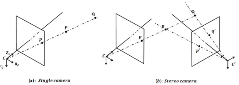
Vision-based techniques are also classified in [23] according to the vision sensor configuration. Most systems are based on a single (monocular) camera [12] [16] [17] [24] [25] [26] or two cameras. In this case, the cameras are generally mounted so that their fields of view overlap and form a stereo or binocular camera [15] [27] [28] [29]. With a monocular camera, motion parameters are provided up to a scale factor. The scale factor is the result of the camera 3D-2D transformation. Indeed, a 2D point in the image plane is the projection of an infinite number of 3D world points, as illustrated in Figure 3.a. Consequently, given a 2D image point, it is not possible to identify the corresponding world point using a single camera. To overcome the scale factor problem, binocular cameras are used. This allows finding the 3D coordinates of the world point using the triangulation technique illustrated in Figure 3.b, based on the knowledge of the baseline between the two cameras. However, the disadvantage of stereo cameras compared to monocular cameras is mainly due to the additional software and hardware cost. In addition, in large-scale environments, the images captured by the camera might contain objects placed too far. Processing these images does not allow recovering the depth values

7

unless the stereo camera baseline is of few metres [30]. This is generally not feasible in the case of small platforms such as mini Unmanned Aerial Vehicles.

Figure 3 : single and stereo camera 3D – 2D transformation

Trinocular (three cameras) configurations also exist but are mainly used in underwater vehicle localization given the difficulties encountered in underwater environments [31]. Moreover, omnidirectional cameras can be used to improve localization performance [18] [24], since omnidirectional vision can overcome the drawbacks of a limited field of view and the short-term feature tracking of traditional cameras by using lenses, mirrors or combinations of cameras to view large surrounding areas. Furthermore, these cameras improve localization accuracy by reducing the perceptual aliasing, increasing robustness to occlusions and decreasing sensitivity to noise w.r.t. traditional cameras [32]. Optical scanning systems using optical laser measurements are also used in localization as detailed in [33]. These systems have the advantage of operating in poor illumination.

Localization techniques depend also on the type of vehicle to localize. Indeed, estimating an Aerial Vehicle pose [34], which usually has a six Degrees of Freedom (DoF) motion (three for rotation and three for translation), is quite different from localizing a Ground Vehicle for which assumptions can be made to reduce the number of DoF, hence simplifying the localization process and increasing the accuracy. For example, in [24] the Ackermann Steering principle describes ground vehicle motion by two DoF, namely the rotation angle and the radius of curvature instead of six.

Vision-based localization techniques depend also on the way the camera is mounted on the vehicle to localize. For ground vehicles, there are four possible installations: a forward-looking camera [25], a downward-facing camera [26], a down-tilted camera [35] [30] and an upward-looking camera. The forward-looking camera provides a high number of landmarks thus allowing good motion estimation accuracy, if landmarks are close to the camera. However, in large-scale environments, the depth information is badly recovered. Additionally, in poor illumination, this method is not feasible. These problems are overcome using a downward facing camera looking at the ground texture and a light source next to the camera. However, downward-facing camera performance is degraded in high dynamics and may not provide a sufficient number of landmarks. The tilted camera provides a larger field of view than the downward-facing camera and

8

captures the ground texture, but captures the vehicle shadow which looks stationary and provides erroneous information about the vehicle motion. Upward-looking cameras are mainly used in indoor environments and exploit the characteristics of this environment such as corners, lamps and door features to localize the robot as explained in [17].

All previous classifications deal with vision as a standalone localization tool. However, previous classifications did not address an important category of localization techniques using visual information. Indeed, the use of visual information within a multi-sensor system is increasingly studied. This sensor integration benefits from the advantages of the different sensors used in the integration scheme and compensates their weakness as described in [36] [37] [38] [39] [40]. This is why, in this paper, our classification is based on the use of the vision sensor as the only localization sensor or as an element of a multi-sensor system as explained in Figure 4. This classification aims to understand the principle of vision-based localization, by comparing the techniques in terms of inputs, outputs, performance, limitations of using only vision for localization and the possible solutions found in the literature to overcome these limitations, namely sensor fusion.

Figure 4 : Proposed classification of vision-based localization techniques

4 Vision as a standalone localization tool in unknown environments

As described above in [11], the main techniques used to localize a device in unknown environments are techniques with no prior information about the environments. This is why, position estimation in such environments using only a camera are based on the Dead-Reckoning principle. The dead-reckoning position solution is defined in [5] as the sum of a series of relative position measurements between consecutive images. Dead-reckoning measures the pose change by comparing

9

two successive images taken from two different places as the device moves, and adds this change to the previous pose to obtain the current pose. This principle is called ‘Visual Odometry’ (VO) in the computer vision community and is defined as the process of incrementally estimating a device pose by examining the changes that motion induces on images taken by its on-board cameras. Pose estimation is performed w.r.t. the world frame and requires the knowledge of the initial pose. We deduce, given this principle and the previous classification criteria, that vision-only position estimation is a local localization technique according to [21]. It is based on either SLAM techniques, which aim to estimate the camera pose jointly with reconstructing the 3D scene by estimating the location of the observed features, or Mapless techniques, which only estimate incrementally the camera pose, namely OF and FT techniques, according to [11].

However, although OF and FT techniques aim to estimate the change in position and attitude between images, they can also include a reconstruction of the 3D scene. Therefore, these techniques may be used as part of the SLAM process and cannot always be considered Mapless techniques. Consequently, rather than distinguishing Map-based and Mapless Techniques, our classification distinguishes between VO that aims to estimate only the camera pose according to the displacement measured from a sequence of camera images without reconstructing the 3D scene, and SLAM that accounts for the correlations existing between camera pose and 3D points observed by the camera and estimates a map of the environment jointly with the camera pose inside this map.

To process VO or Visual SLAM, some assumptions have to be made. First of all, the environment must be sufficiently illuminated. Then, it is important to have static objects dominant over moving objects in the image sequence, because the pose estimation is based on the changes occurring in the images when the device moves, which are computed starting from the recognized static objects. Finally, the overlap between consecutive frames must be sufficient to gather enough information about the displacement.

4.1 Visual Odometry

VO generally relies on 3 main steps: establishing matches between two frames, removing outliers and estimating the motion between the two frames.

- Establishing matches

Matching two frames may be performed either by OF or by FT. FT is considered by [41] as a sparse OF where the considered pixels are selected wisely. According to [41], FT is preferable to OF since the pixel selection provides more robustness against noise.

10

Optical Flow

OF is the apparent motion of features in a sequence of images. When the device moves, static features appear to be moving with respect to the device. The OF between two consecutive frames is represented by a set of vectors, one for each pixel, where their norm depends on the motion speed and their directions represent the movement of the corresponding pixel in consecutive images. In the monocular case, the norm of these vectors is estimated up to a scale factor. To estimate OF at all pixels, the ‘Intensity Constancy’ assumption, which states that the intensity of a small image region remains constant with time, is used. This assumption is formulated by:

(6)

where is the point intensity at time epoch and is the displacement in the image plane of this point between and . Many approaches have been proposed in the literature to solve the equation and find the displacement [42]. This vector is then converted from the image plane to the camera frame and afterwards to the world frame. One method to derive odometry using OF was presented in [35]. This method uses a single camera mounted on top of a robot and tilted downwards to film the ground. The images taken by this camera are sub-divided into three regions: ground, horizon, and sky. The OF vectors calculated from the ground region estimate robot translational motion, those calculated from the sky region estimate the rotation and those near the horizon are discarded.

Feature Tracking

The first step in FT is to detect salient zones (corners, edges, etc.) in the current image called Features. Feature detectors must be sufficiently robust to a perspective change following the camera motion, in order to detect the same points in all images. The most widely used detectors are the Harris corner detection algorithm [43] and the Shi and Thomasi corner detection algorithm [44].

Once detected, these features have to be characterized in a unique way. This second step in FT is performed through feature description. A feature descriptor includes all feature characteristics. A very large number of feature descriptors have been developed. The most widely used algorithms are Scale Invariant Feature Transform (SIFT) [45] and Speeded Up Robust Feature (SURF) [46]. An evaluation of feature detectors and descriptors is performed in [47].

Besides corner points, lines are also used as features especially in indoor environments where geometrical structures having parallel or perpendicular edges like walls, doors and windows are widely found. Line detection can be performed using different techniques such as Hough transform, Iteratively-Reweighted-Least Squares-based line detection, Edge Linking Method or Line Fitting Using Connected Components described and compared in [48]. A method of attitude

11

estimation is described in [48], where the attitude is deduced from the change in the configuration of projected lines in the camera image when the camera moves.

The final step of FT is Feature Matching which can be performed in two ways: either by extracting features from both previous and current images independently, then performing matching, or by extracting features from the previous image, predicting the regions where the features could be found in the current image and then performing matching. The former approach is more suitable for large-scale environments while the latter approach is generally used in small-scale environments. The goal of this step is to match the features that correspond to the same physical feature existing in the camera field of view in both previous and current image. This phase consists of computing a matching score that indicates the likelihood that two features correspond to the same physical feature. The features that have the highest scores are matched. The matching process can also be performed considering the computation of the distance between the descriptors of the features. In this case, the features having the smallest distances are matched.

- Outlier Removal

The second step of VO is a process applied to exclude wrong matches usually called outliers. These wrong matches can cause significant error in estimating camera motion and removing them is necessary to obtain accurate motion estimation. To exclude wrong matches, the algorithm usually used is RANdom SAmple Consensus (RANSAC) [49], based on the epipolar geometry constraint described in Figure 5. Epipolar geometry defines the geometrical constraints between two different views of the same 3D point. Denoting and the image points corresponding to the same 3D point viewed from different locations, then , , and camera centres lie all in the same plane [50]. Based on this principle, all corresponding image points satisfy the coplanarity equation:

(7)

Where is called the Fundamental Matrix. expresses the camera motion from to and the internal camera calibration. Each pair of points and adds a constraint on the fundamental matrix estimation. The normalized 8-point algorithm described in [50] is used to estimate using RANSAC algorithm for robustness against outliers. This means that to estimate , at least 8 pairs of points must be correctly matched. If the camera is calibrated, i.e. the calibration matrix is known, then the coplanarity equation is given by:

̂ _̂ (8)

Where ̂ , ̂ and is called the Essential Matrix. E is the specialization of the fundamental matrix to the case of known calibration parameters. At least 5 pairs of points must be correctly matched to estimate E, using the 5-point algorithm addressed in [51].

12

Figure 5 : Epipolar constraints [50]

- Motion estimation

The camera motion between the current image and the previous image is estimated based on the matches established in the previous steps. The trajectory of the camera is recovered by concatenation of all these single movements. In the case of unknown intrinsic parameters, only the fundamental matrix is estimated. The camera displacement is recovered up to a projective transformation, and it is not possible to recover the distance ratios and the angles. That is why, in most of VO applications, the camera is assumed to be calibrated, i.e. the calibration matrix K is known. In this case, the essential matrix is computed using equation 8. It has been shown in [50] that the essential matrix can be decomposed into a rotation and a translation vector such as:

[ ] (9)

Where [ ] is the skew-symmetric matrix of and is the translation vector up to a scale factor [37].

A complete explanation of VO is detailed in [52] and [53].

4.2 Simultaneous Localization And Mapping (SLAM)

The Simultaneous Localization And Mapping (SLAM) is a process by which a mobile device builds the map of an environment and uses this map at the same time to deduce its location in it. In SLAM, both the device trajectory and the location of all landmarks are estimated online without requiring any a priori location knowledge. The first SLAM approaches used different sensors such as Laser Scanner [54], Radar [13], Sonar [55], odometric data provided by Wheel Speed Sensors, or multi-sensor data fusion [36]. With the recent developments in vision-based techniques, cameras have been used as sensors making vision-based SLAM more and more attractive. Pioneering work on real-time visual SLAM has been carried out first by [12]. Contrary to VO which aims to estimate only the camera pose based on the displacement measured between two successive frames, vision-based SLAM accounts for the correlations that exist

13

between the camera pose and the 3D position of the observed features and is therefore more accurate than VO but requires a higher computational complexity. Visual SLAM uses the same techniques as VO, but differs in its aim to localize and build a map (determine the 3D feature positions) simultaneously, instead of only localizing. This improves dramatically the pose estimation accuracy since it takes into account the correlation between the observed features and the camera pose, but at the cost of an additional computational burden. Consequently, the choice between visual SLAM and VO depends on the trade-off between accuracy and simplicity in implementation.

In [14], vision-based SLAM techniques are classified into two categories: a stereovision approach, in which 3D point positions are fully observed from a single position, and a bearing-only approach that exploits monocular sequences. Visual SLAM techniques are also subdivided according to [56] into keyframe-based SLAM and filtering-based SLAM.

- Keyframe-based visual SLAM

If no a priori knowledge of the scene is provided, estimation of the camera pose is completely correlated with estimating the 3D locations of the observed feature known as 3D scene reconstruction. This is referred to as the Structure From Motion (SFM) problem. The principle of Keyframe-based SLAM is to compute the camera pose given the position of the already reconstructed 3D map points, to reconstruct new 3D points if necessary and to refine jointly the 3D reconstructed points and the camera pose for some selected keyframes from the sequence. This approach is based on Bundle Adjustment (BA) [57] which is a nonlinear least squares refinement that aims to minimize the reprojection error defined as the sum of squared residuals between the points detected in the images and the reprojections obtained from the calculated model, thus improving the positioning accuracy. For a state of the art of BA algorithms please refer to [58].

In this case, instead of establishing matches between features detected in successive images called (2D/2D correspondence), visual SLAM establishes matches between detected features in the current image and already reconstructed features. This process described in [52] is called ‘3D/2D correspondence’. The motion estimation is not deduced from the decomposition of the essential matrix such as in VO, but rather from solving the Perspective-Three-Point Problem. The definition and the solutions of this problem are detailed in [59].

- Filtering-based visual SLAM

This approach is based on the construction of a probabilistic 3D feature map, describing the current pose estimation of the camera and the reconstructed 3D features that define the map, in the world frame. In addition, this approach provides the estimate uncertainties. The map is initialized in the beginning of the process and is updated, as the device moves, by Bayesian Filters such as Kalman Filter (KF), Extended Kalman Filter (EKF) or Particle Filter (PF). The probabilistic map is mathematically described through a state vector and a covariance matrix. The state vector comprises the concatenation

14

of the estimations of the camera pose and the 3D features. The probability density function of the map parameters is usually approximated by a multiple variable Gaussian distribution.

- Optimal approach for Visual SLAM

Ii is difficult to compare the keyframe-based SLAM and the filtering based SLAM and to conclude which approach is better. In fact, each approach has its advantages and drawbacks, depending on the intended application. Filtering-based visual SLAM has the advantage of handling easily measurement covariances, but is less accurate than keyframe SLAM in large-scale environments [60]. An analysis of the performance of keyframe-based and filtering-based approaches is performed in [56]. It revealed that the keyframe-based approach with BA is more efficient than the filtering-based approach in terms of accuracy and computational cost.

4.3 Limits of standalone visual localization techniques

It should be noted that vision-based localisation techniques suffer from the accumulated error resulting from the use of the dead-reckoning principle. Compared to SLAM, VO suffers from a higher drift rate because VO techniques are based only on the dead-reckoning principle, whereas SLAM techniques combine dead-reckoning and BA which improves the accuracy of the localization process, but at the cost of an increased computational burden for the optimization process.

In addition, it is important to point out that the knowledge of the geo-referenced position of the camera is impossible if its initial position and attitude are not known in a global frame such as the ECEF frame. Therefore, the use of a global means such as GNSS becomes necessary in this case.

Finally, when choosing a camera configuration, it should also be taken into account that the use of a single camera induces a scale drift within time. Indeed, it is difficult to propagate the scale factor throughout the process, since with a single camera, this scale is not observable during the localization process. Consequently, the scale factor is directly the subject of the accumulated errors and drifts within time, especially when many features disappear abruptly between two successive images (e.g. in sharp turns). For these reasons, the integration of vision-based systems with other sensors is necessary to improve the localization performances.

5 Multi sensor localization

The objective of sensor fusion is to improve the performance obtained by each sensor taken individually by combining their information. We generally consider three different ways to combine sensor measurements to estimate the navigation solution, which vary depending on the information exchanged by the sensors and the integration engine: loose-coupling, tight-coupling, deep-coupling. With loose-coupling, each sensor provides a positioning solution. The hybridized solution

15

is the combination of different solutions provided by each sensor individually. With tight and deep coupling, fusion of sensor information takes place before positioning solution estimation. Tight architectures combine the sensors information to provide a unique solution, while in deep architectures, the sensors work as a unique system and fusion is performed inside one of the sensors processes. To our knowledge, deep-coupling with vision aid has not yet been addressed.

The most widely used filter for sensor fusion is the EKF. PF is also used to fuse visual information with other sensors. Visual SLAM fusion with inertial measurements using the PF has been addressed in [61] [62] [63]. In [63], a comparison between the EKF and the PF shows that EKF provides a higher precision. The fusion of visual information with other sensors could also be done within a BA framework. The following sections detail examples of visual information fusion with other sensors (Focus is on EKF and BA framework fusion).

5.1 INS and Camera Fusion

The fusion of INS and visual information, also called ‘Vision-aided Inertial Navigation’ aims to combine INS and vision advantages, while balancing the system drawbacks. Inertial sensors have a large measurement uncertainty when in slow motion and lower relative uncertainty at high velocities, while cameras can track features very accurately at low velocities and less accurately with increasing velocity. Furthermore, in the absence of GNSS information, the INS solution drifts over time that may be reduced by the vision sensor [38].

Starting with early work such as [64], there is now growing interest in fusing inertial and visual sensor. As explained in Section 4, INS/camera fusion may follow either the SLAM principle (estimation of the current camera position and attitude, and the 3D position of the observed landmarks jointly) or the VO principle (estimation of only the camera position and attitude).

In [65] and [66], a monocular SLAM is used and a loosely-coupled approach that fuses inertial and visual data is implemented. The SLAM algorithm is based on a keyframe approach as described in [67]. It outputs camera poses and 3D position of the observed landmarks up to a scale factor. These approaches estimate the scale factor by fusing the visual and inertial measurements through an EKF by putting the scale as an additional variable in the state vector.

In [40], a tightly-coupled INS/binocular camera fusion is used for aircraft position, velocity and attitude estimation. This approach is based on the use of measurements obtained by the knowledge of the 3D position of tracked features. In fact, once features are identified in the current image, the system predicts where these features should appear in the next image based on the inertial measurements, to constrain the search space within the next image during the matching process, as

16

described in Figure 6. The state vector is given by the INS and consists of the device position, velocity and orientation w.r.t. the world frame.

Figure 6: Feature projection [40]

Once feature matches are determined, the errors between the predicted feature location and the actual feature location are used to correct errors in the state vector. This is achieved in [40] using an EKF described in Figure 7. In this filter, the locations of stationary objects are tracked and used to estimate and update the errors in the inertial navigation system. The inertial navigation system is, in turn, used to support the FT loop.

Figure 7 : Image-aided inertial navigation filter block diagram [40]

The comparison between the vision-aided INS and the standalone INS performances, carried out in [40], shows that over 10 minutes, the use of vision measurements improves the errors by many orders of magnitude.

A different tightly-coupled approach for vision-aided inertial navigation is proposed in [68]. To estimate the position, velocity and attitude of a ground vehicle, an error state EKF-based estimation algorithm for real-time navigation is used.

17

The filter state vector describes the evolving Inertial Measurement Unit (IMU) state augmented with the current estimate of the camera pose when an image is taken, based on the IMU pose. The measurement model expresses the geometric constraints that arise when a static feature is observed from multiple camera poses. The observed features are tracked between previous camera poses, and used to update the vehicle state. This measurement model does not require including 3D feature positions in the state vector of the EKF thus reducing the computational complexity for real-time application. Experimental results show a good performance of the system since the error is of 0.31% of the travelled distance.

In [69], a photogrammetric approach is addressed for land vehicle pose estimation. INS/stereo vision fusion is only used during GPS outages to reduce INS drifts. When GPS signals are available, pose estimation is performed through the classical GPS/INS integration and stereo vision is only used to determine 3D locations of the features in the image sequence exploiting the vehicle pose obtained by the GPS/INS system. When the GPS is no longer available, the pose parameters are computed using INS and extracted features only. In this case, 3D coordinates of the feature points are calculated for the last stereo frame captured before GPS outage. Upon the next image acquisition, features corresponding to previously triangulated features are identified and the vehicle location is updated using their position and the inverse 3D coordinate computation. This procedure is repeated until the GPS signals become available again. Simulations carried out show that in one minute GPS outage, errors from pure INS solution grow up to 70 meters, while errors after integrating INS data and image information are below 1.9 meters.

5.2 GNSS and Camera Fusion

As for any GPS/INS fusion scheme, the goal of integrating GPS and visual information is to compensate for their limitations and to benefit from their complementarities. In fact, a standalone GNSS navigation solution is generally not feasible in challenging environments such as urban canyons, where nevertheless a set of one or two GNSS signals may be still available, whereas visual information can work efficiently in these environments if a lighting source is available. On the other hand, visual information suffers from the drift due to the dead-reckoning principle, as well as a scale factor in the monocular case, while GNSS systems have in turn bounded errors.

In [39], a loosely-coupled GPS/VO integration scheme is presented following the classic loosely GPS/INS integration as described in Figure 8. It assumes that if a monocular camera is used, then the scale factor can be recovered. The KF estimates the errors of the navigation solution provided by the camera, using the difference between GPS and camera solutions as the measurement to the KF. The errors estimated by the KF are used to correct the camera solution.

18

Figure 8: GPS/VO Error State Filter [39]

The tightly-coupled approach is addressed by [70] to estimate a 6 DoF pose in environments where a GNSS-only solution is not feasible. A method for combining limited GPS carrier phase measurements with features extracted from images of a monocular video camera is proposed. The GPS carrier phase measurements are used to overcome the scale factor problem due to the use of a monocular camera. The estimation procedure aims to compute the device pose changes between two images, and ranges to the observed features. The fusion is performed in two equations defining the relationship between the device range to features and its pose change and one equation expressing the relationship between the carrier phase and position changes. In [70], these equations are resolved using the Least Mean Square Estimate. The experimental results carried out in [70] show that the GPS position change estimation from carrier phase measurements, if at least 4 satellites are available and under open sky, is accurate at a millimetre level, whereas when 3 GPS carrier phase measurements are available, the GPS-video integration achieves a positioning accuracy of a centimetre to sub-decimetre level and provides a heading accuracy in a range of 1 to 3 degrees.

The fusion of GNSS and monocular SLAM within a BA framework is addressed in [71], through a BA with inequality constraint (IBA). The reprojection error is computed based on both the camera and GPS poses. The fusion is performed only if it does not degrade too much the reprojection error, i.e. if the degradation of the reprojection error does not exceed a threshold slightly greater than the minimum reprojection error. Results show that IBA is robust for in-plane localization. Its performance is similar to that of the GPS. However it is not appropriate for a 6 DoF localization, since it may increase drifts on the device’s altitude and orientation.

5.3 GNSS, Camera and INS Fusion

The GNSS, camera and INS fusion is widely used in environments where GNSS signals are not always available, such as urban canyons.

In [37], the integration of a Strapdown IMU, a GNSS and a camera is performed in order to estimate the position, velocity and attitude of a ground vehicle. The vision system based on a monocular camera estimates the vehicle rotation

19

and translation up to a scale factor, using VO techniques. This scale factor is resolved using the GNSS data. At least, two satellites in view are required. Between camera/GNSS data update, the vehicle motion is estimated by strapdown IMU mechanization. Once new camera/GNSS measurement data arrive, all derived navigation information is transformed in order to enable the EKF engine for accurate navigation solution and IMU sensor calibration. The system is described in Figure 9. The simulations carried out show that the positioning accuracy using this system is significantly improved in GPS outages.

Figure 9: The EKF-based architecture [37]

In [34], a tightly-coupled and feed-forward EKF is proposed to estimate the position, velocity and attitude of an aircraft. The filter combines inertial, visual and GPS measurements if GPS is available and combines inertial and visual measurements during GPS outages. The EKF estimates the errors in the navigation state produced by the INS using visual and GPS measurements. Unlike classical approaches where vision provides variables of interest (position, attitude, etc.), this approach uses vision as an aiding source providing raw data from the images as measurements to the navigation algorithm. The visual raw measurements describe the pointing vector from the aircraft to a target of unknown location. The errors estimated by the EKF are removed from the INS state to provide the final estimated position, velocity and attitude. The integration architecture is described in Figure 10.

20

Figure 10 : Overall Integration Architecture [34]

It is shown in [34] that using this configuration, the navigation position error is improved by 70% over the free inertial solution for a 400 second GPS outage.

A different solution to integrate video, INS and GPS is proposed in [72] . The INS and video are tightly-coupled. The filter state vector describes the evolving IMU state and the measurement model is based on the reprojection error of the

observed features on the camera’s image plane. Since the vision-aided inertial navigation algorithm performs only dead

reckoning, a global position is calculated by a GPS.. The experimental results show that the localization mean error of the system computed over 10 minutes does not exceed 1meter, outperforming the standalone GPS performance.

5.4 Odometer and Camera Fusion

In [73], an odometer aids the monocular visual SLAM within a BA framework. The idea is to change BA by substituting the estimated 3D camera position (the orientation is kept unchanged) by a corrected one ̃ , each time a new keyframe is acquired. The correction provided by equation 10 is performed by the odometer which estimates the scale factor.

̃ ‖ _‖

(10)

where ‖ ‖ is the Euclidean norm, and is the distance travelled between and , estimated by the odometer.

Simulations carried out in [73] show that this system provides an improvement of about 10 orders of magnitude in the positioning accuracy, and a significant improvement in the attitude accuracy.

In [60], a multi-sensor architecture within a BA framework is performed. Here, a second sensor modifies the monocular SLAM algorithm in order to reduce the drift of the system. It predicts the system pose, and this prediction is used to make a constraint on the system displacement, improving the BA refinement process by minimizing a weighted sum of

21

the two sensors terms instead of only minimizing the camera terms. This proposition is validated with two types of sensors, an odometer embedded in a vehicle and a gyroscope integrated in an IMU and carried by a pedestrian. Results show an improvement, for both sensors, of the localization accuracy using the multi-sensor architecture, compared to the classical BA based only on visual information.

5.5 INS, Odometer and Camera Fusion

In the case of ground vehicles, the use of odometer data has been identified as one of the most attractive sensors. An INS/odometer/omnidirectional camera integration scheme is proposed in [74]. The proposed visual system extracts and tracks Vanishing Points (Vanishing Points refer to the intersection of the projection of world parallel lines in the image) in omnidirectional images to estimate the vehicle rotation and thus improves the performance of INS/odometer system, in the case of GPS outages, by limiting its drift. The integration is performed by an error-based KF. The state vector comprises the position, velocity and attitude errors, the gyro drifts, the accelerometer biases and the camera errors. The KF compares the INS output with data acquired from camera and odometer. Therefore two types of measurements are utilized for the measurement update of the KF during GPS outages: the attitude derived from the camera and the speed derived from the odometer. A comparison between the INS/odometer and the proposed vision-aided INS/odometer systems is carried out in [74] during 100s GPS outage, showing that the vision-aided system provides about 30.7% (1.63m to 1.13m), 31.6% (0.99m to 0.67m) and 30.2% (3.19m to 2.23m) improvement in the average, deviation and maximum of the horizontal position error, respectively.

5.6 Summary of Performance Comparison

Table 2 summarizes the performance of the different fusion architectures and techniques surveyed in the previous sections. Since the experimental conditions and the metrics evaluating the proposed architectures are different in each reference, Table 2 describes, for each technique, the experimental conditions and the corresponding metrics.

Technique Environment and

assumptions bias (m) Standard deviation (m) Other metrics Ref. metric Value DG-16

RTK-GPS - Real data CEP50

* _{0.4 m [75]} GPS - Land Vehicle (50 km/h) - 3 km trajectory in urban environment – Real data 2.68 1.38 [76] [77] Monocular constrained BA SLAM 12.82 8.828 GPS + monocular BA SLAM 2.44 2.02

22

GPS carrier phase - Land Vehicle - Open sky - Real data Delta position error millimetre -level [70] GPS carrier phase + video - Land Vehicle (3.6 km/h) - Use of only 3 satellites - Open sky - Real data Delta position error E 1.55 cm N 5.81 cm U 7.87 cm GPS + « Dead Reckoning »: EKF - Land Vehicle - Simulated data 20.71 [78] GPS + « Dead Reckoning » : PF 3.56

GPS+INS - Simulated data Qualitative KF better than PF [79] GPS + INS MEMS EKF (loose) - Land vehicle - 50mn trajectory in dense urban, semi urban, dense trees and clear sky environment - Less than 4 satellites available during 43% of the time - Real data E -5.30 50.22 [80] N 1.20 19.93 U 2.47 -22.82 GPS + INS MEMS EKF (tight) E -0.02 1.75 N 0.24 1.85 U 2.03 -13.92 INS+ visual

SLAM - Real data Qualitative

KF better than PF [63] tactical-grade INS - Aircraft (180 km/h groundspeed) - 1200 s trajectory

- Terrain model uncertainty of 5 metres - Simulated data Horizontal root-sum-squared error ~104 [40] tactical-grade INS + video measurements + terrain model Horizontal root-sum-squared error <100 Monocular BA SLAM - Land vehicle (50km/h) - Urban environment - A 4km sequence in urban environment - Real data 348.89 271.22 [73] Odometer + monocular BA SLAM 33.69 23.14 Medium-grade INS + odometer - Land vehicle - 100 s trajectory - Non-holonomic constraints - Real data h o r i z o n t a l 1.63 0.99 [74] Medium-grade INS + odometer + omnidirectional vision 1.13 0.67

*_{CEP50: Circular ErrorProbable with a probability of 0.5}

23

6 CONCLUSION

Visual navigation has become one of the most promising navigation means given its capability of providing extensive usable information to improve the accuracy of the navigation solution in unknown environments. The objective of this study is to describe and compare recent vision techniques for localization and provide guidelines for the integration of visual information with other navigation measurements such as GNSS or INS. By integrating all sensor information, it is in fact possible to exploit all available information and overcome each sensor difficulties such as signal propagation errors and outages for GNSS, drifts and expensive cost for INS, and drifts and scale factor for monocular vision. As evidenced, all the studies carried on sensor integration show that with visual information, localization accuracy is improved. In the future, activities should focus on improving sensor fusion architectures to get higher localization performance and reduce the computational burden for real-time localization.

ACKNOWLEDGMENTS

This work was done as part of the MIMOSA (SystèMe de navIgation et téléMatique par géolocaliSation et hybridation de cApeturs) project. The authors would like to thank the DGCIS (Direction Générale de la Compétitivité, de l'Industrie et des Services) for funding this project.

REFERENCES

[1]

Groves, P.D.: ‘The PNT Boom. Future Trends in Integrated Navigation’, Inside GNSS, 2013

[2]

Ochieng, W., Sauer, K., Walsh, D., Brodin, G., Griffin, S., Denney, M.: ‘GPS Integrity and Potential Impact

on Aviation Safety’, Journal of Navigation, 2003, 56, (1), pp.5-65

[3]

Morales, Y., Tsubouchi, T.: ‘DGPS, RTK-GPS and StarFire DGPS Performance Under Tree Shading

Environments’, Proc. IEEE Int. Conf. Integration Technology, 2007, pp.519-524

[4]

Soubielle, J., Fijalkow, I., Duvaut, P., Bibaut, A. : ‘GPS Positioning in a Multipath Environment’, IEEE Trans. Signal Processing, 2002, 50, (1), pp.141-150

[5]

Groves, P.D.: ‘Principles of GNSS, Inertial, and Multisensor Integrated Navigation Systems’, 2008

[6]

Brown, A.K.: ‘Test Results of a GPS/Inertial Navigation System Using a Low Cost MEMS IMU ’, Proc. 11th

Annual Saint Petersburg International Conf. Integrated Navigation System, 2004

[7]

Skog, I., Handel, P.: ‘In-Car positioning Navigation and Technologies – A survey’, IEEE Trans. Intelligent Transportation Systems, 2009, 10, (1), pp.4-21

24

[8]

Nistér, D., Naroditsky, O., Bergen, J.: ‘Visual odometry for ground vehicle applications’, Journal of Field Robotics, 2006, 23, (1), pp.3-20

[9]

Engel, J., Sturm, J., Cremers, D.: ‘Camera-based navigation of a low-cost quadrocopter’, Proc. Int. Conf.

Intelligent Robot Systems, 2012

[10]

DeZousa G.N., Kak A.C.: ‘Vision for mobile robot navigation: A survey’, IEEE Trans. Pattern Analysis and

Machine Intelligence, 2002, 24, (2), pp.237-267

[11]

Bonin-Font, F., Ortiz, A., Oliver, G.: ‘Visual Navigation for Mobile Robots: A Survey’, Journal of Intelligent and Robotic Systems, 2008, 53, (3), pp.263-296

[12]

Davison, A.J., Reid, I.D., Molton, N.D., Stasse, O.: ‘Vision for mobile robot navigation: A survey’, IEEE Trans. Pattern Analysis and Machine Intelligence, 2007, 29, (6), pp.1052-1067

[13]

Dissanayake, M.W.M.G., Newman, P., Clark, S., Durrant-Whyte, H.F., Csorba, M.: ‘A Solution to the Simultaneous Localisation and Map-Building Problem’, IEEE Trans. Robotic and Automation, 2001, 17, (3), pp.229-241

[14]

Lemaire, T., Berger, C., Jung, I.K., Lacroix, S.: ‘Vision-Based SLAM: Stereo and Monocular Approaches’, International Journal of Computer Vision, 2007, 74, (3), pp.343–364

[15]

Jung, I.K.: ’Simultaneous Localization and Mapping in 3D Environments with Stereovision’, PhD thesis, INP

Toulouse, 2005

[16]

Celik, K., Chung, S., Somani, A.: ‘Mono-vision corner slam for indoor navigation’, Proc. IEEE Int.

Electro/Inform. Technol., 2008, pp.343-348

[17]

Hwang S.Y., Song, J.B.: ‘Monocular vision-based SLAM in indoor environment using corner, lamp, and door

features from upward-looking camera’, IEEE Trans. Ind. Electron., 2011, 58, (10), pp.4804-4812

[18]

Winters, N., Santos-Victor, J.: ‘Omni-directional Visual Navigation’, Proc. Int. Symp. Intelligent Robotics Systems, 1999, pp.109-118

[19]

Ulrich, I., Nourbakhsh, I.: ‘Appearance-based place recognition for topological localization’, Proc. IEEE Int.

Conf. Robotics and Automation, 2000, pp.1023-1029

[20]

Segvic, S., Remazeilles, A., Diosi, A., Chaumette, F.: ‘Large-Scale Vision-based Navigation Without an

Accurate Global Reconstruction’, Proc. IEEE Conf. Computer Vision and Pattern Recognition, 2007, pp.1-8

[21]

Se, S., Lowe, D.G., Little, J.J.: ‘Vision-based Global Localization and Mapping for Mobile Robots’, IEEE Trans. Robotics, 2005, 21, (3), pp.364-375

25

[22]

Zhang, W., Kosecka, J.: ‘Image Based Localization in Urban Environments’, Proc. IEEE Int. Symp. 3D Data

Processing, Visualization, and Transmission, 2006, pp.33-40

[23]

Kitt, B.M., Rehder, J., Chambers, A.D., Schonbein, M., Lategahn, H., Singh,S.: ‘Monocular Visual Odometry

using a Planar Road Model to Solve Scale Ambiguity’, Proc. European Conf. Mobile Robots, 2011

[24]

Scaramuzza, D.: ‘1-Point-RANSAC Structure from Motion for Vehicle-Mounted Cameras by Exploiting

Non-holonomic Constraints’, International Journal of Computer Vision, 2011, 95, (1), pp.74-85

[25]

Choi, S., Joung, J.H., Yu, W., Cho, J.I.: ‘What does ground tell us? Monocular visual odometry under planar

motion constraint’, Proc. IEEE Int. conf. Control, Automation and Systems (ICCAS), 2011, pp.1480-1485

[26]

Nourani-Vatani, N., Vincius, P., Borges, K.: ‘Correlation-based Visual Odometry for Ground Vehicles’, Journal of Field Robotics, 2011, 28, (5), pp.742-768

[27]

Sunderhauf, N., Protzel, P.: ‘Stereo Odometry – A review of approaches’, Technical Report 3/07, Institute of

Automation, Dep. Electrical Engineering and Information Technology, Chemnitz University of Technology

[28]

Agrawal, M., Konolige, K., Iocchi, L.: ‘Real-Time Detection of Independent Motion using Stereo’, IEEE

Workshops Application of Computer vision, 2005, pp.207-214

[29]

Takezawa, S., Herath, D.C., Dissanayake, G.: ‘SLAM in Indoor Environments with Stereo Vision’, IEEE/RSJ

Int. Conf. Intelligent Robots and Systems, 2004, pp.1866-1871

[30]

Hong, S., Song, J.B., Baek, J.H., Ryu, J.K.: ‘Visual odometry for outdoor environment using a

downward-tilting camera and self-shadow removal algorithm’, Proc. IEEE Int. Conf. Control, Automation and Systems (ICCAS), 2012, pp.960-963

[31]

Dudek, G., Jenkin, M., Prahacs, C., et al: ‘A Visually Guided Swimming Robot’, Proc. IEEE Int. Conf. Intelligent Robots and Systems, 2005, pp.3604-3609

[32]

Zhang, Y., Cao, J., Lou, L., Su, B.: ‘Appearance-based mobile robot navigation using omnidirectional

camera’, Proc. IEEE Int. Conf. Fuzzy Systems and Knowledge Discovery, 2012, pp.2357-2361

[33]

Básaca-Preciado, L.C., Sergiyenko, O.Y., Rodríguez-Quinonez, J.C., et al: ‘Optical 3D laser measurement

system for navigation of autonomous mobile robot’, Optics and Lasers in Engineering Journal, 2014, 54,

pp.159-169

[34]

Raquet, J.F., Giebner, M.: ‘Navigation Using Optical Measurements of Objects at Unknown Locations’, Proc.

Annual Meeting of ION and CIGTF 22nd Guidance Test Symposium, 2003, pp.282-290

26

System Using Consumer-grade Monocular Vision’, Proc. IEEE Int. Conf. Robotics and Automation, 2005, pp.3421-3427

[36]

Castellanos, J., Martinez, J., Neira, J., Tard s, J.: ‘Simultaneous Map Building and Localization for Mobile

Robots: A Multisensor Fusion Approach’, Proc. IEEE Int. Conf. Robotics and Automation, 1998,

pp.1244-1249

[37]

Chu, T., Guo, N., Backén, S., Akos, D.: ‘Monocular Camera/IMU/GNSS Integration for Ground Vehicle

Navigation in Challenging GNSS Environments’, Sensors, 2012, 12, (3), pp.3162-3185

[38]

Corke, P., Lobo, J., Dias, J.: ‘An Introduction to inertial and visual sensing’, International Journal of Robotics

Research, 2007, 26, (6), pp.519-535

[39]

Dusha, D., Mejias, L.: ‘Attitude observability of a loosely-coupled GPS/Visual Odometry Integrated

Navigation Filter’, Proc. Australasian Conf. Robotics and Automation, 2010

[40]

Veth, M.: ‘Fusion of Imaging and Inertial Sensors for Navigation’, PhD thesis, Air Force Institute of

Technology, 2006

[41]

Nourani-Vatani, N., Borges, P.V.K., Roberts, J.M. : ‘A Study of Feature Extraction Algorithms for Optical

Flow Tracking’, Proc. Australian Conf. Robotics and Automation, 2012

[42]

Barron, J.L., Fleet, D.J., Beauchemin, S.S., Burkitt, T.A. : ‘Performance of optical flow techniques’, Proc. IEEE Computer Society Conf. Computer Vision and Pattern Recognition, 1992, pp.236-242

[43]

Harris, C., Stephens, M.: ‘A Combined Corner and Edge Detector’, Proc. Alvey Vision Conference, 1988,

pp.147-151

[44]

Shi, J., Tomasi, C.: ‘Good Features to track’, Proc. IEEE Computer Society Conf. Computer Vision and Pattern Recognition, 1994, pp.593-600

[45]

Lowe, D.G.: ‘Distinctive Image Features from Scale-Invariant Keypoints’, International Journal of Computer

Vision, 2004, 60, (2), pp.91-110

[46]

Bay, H., Ess, A., Tuytelaars, T., Van-Gool, L.: ‘SURF: Speeded-Up Robust Features’, Computer Vision and Image Understanding, 2008, 110, (3), pp.346-359

[47]

Gauglitz, S., Höllerer, T., Turk, M.: ‘Evaluation of Interest Point Detectors and Feature Descriptors for Visual

Tracking’, international Journal of Computer vision, 2011, 94, (3), pp.335-360

[48]

Kessler, C., Ascher, C., Frietsch, N., Weinmann, M., Trommer, G.: ‘Vision-based attitude estimation for

27

[49]

Choi, S., Kim, T., Yu, W.: ‘Performance Evaluation of RANSAC Family’, Proc. British Machine Vision

Conference, 2009

[50]

Hartley, R., Zisserman, A.: ‘Multiple View Geometry in Computer Vision’, (Cambridge University Press,

March 2004, 2nd edn.), pp.239-261

[51]

Nistér, D.: ‘An Efficient Solution to the Five-point Relative Pose Problem’, IEEE Trans. Pattern Analysis and

Machine Intelligence, 2004, 26, (6), pp.756-770

[52]

Scaramuzza, D., Fraundorfer, F.: ‘Visual Odometry Part I: The First 30 Years and Fundamentals’, IEEE Trans.

Robotics and Automation Magazine , 2011, 18, (4), pp.80-92

[53]

Fraundorfer, F., Scaramuzza, D.: ‘Visual Odometry Part II: Matching, Robustness, Optimization, and

Applications’ , IEEE Trans. Robotics and Automation Magazine , 2012, 19, (2), pp.78-90

[54]

Castellanos, J.A, Montiel, J.M.M., Neira, J., Tardos, J.D.: ‘A Probabilistic Framework for Simultaneous

Localization and Map Building’, IEEE Trans. Robotics and Automation, 1999, 15, (5), pp.948-952

[55]

Tardos, J.D., Neira, J., Newman, P.M., Leonard, J.J,: ‘Robust Mapping and Localization in Indoor Environments Using Sonar Data’, International Journal of Robotics Research, 2002, 21, (4), pp.311-330

[56]

Strasdat, H., Montiel, J.M.M, Davison, A.J.: ‘Visual SLAM: Why Filter?’, Image and Vision Computing,

2012, 30, (2), pp.65-77

[57]

Engles, C., Stewénius, H., Nistér, D.: ‘Bundle adjustment rules’, Proc. Symp. Photogrammetric Computer Vision, 2006

[58]

Triggs, B., McLauchlan, P.F., Hartley, R.I, Fitzgibbon, A.W.: ‘Bundle Adjustment - A Modern Synthesis’,

Proc. Int. Workshop Vision Algorithms: Theory and Practice, Springer-Verlag, 1999

[59]

Haralick, R.M., Lee, D., Ottenburg, K., Nolle, M.: ‘Analysis and solutions of the three point perspective pose

estimation problem’, Proc. IEEE Computer Society Conf. Computer Vision and Pattern Recognition, 1991,

pp.592-598

[60]

Michot, J., Bartoli, A., Gaspard, F.: ‘Bi-objective Bundle Adjustment with Application to Multi-sensor

SLAM’, In 3DPVT, 2010

[61]

Schon, T.B., Karlsson, R., Tornqvist, D., Gustafsson, F.: ‘A Framework For Simultaneous Localization and

Mapping Utilizing Model Structure’, Proc IEEE Int. Conf. Information Fusion, 2007, pp.1-8

[62]

Karlsson, R., Schon, T., Tornqvist, D., Conte, G., Gustafsson, F.: ‘Utilizing model structure for efficient

28

pp.1-10

[63]

Bleser, G., Strickery, D.: ‘Using the marginalised particle filter for real-time visual-inertial sensor fusion’,

Proc. IEEE/ACM. Int. Symp. Mixed and Augmented Reality, 2008, pp.3-12

[64]

Viéville, T., Faugeras, O.D.: ‘Cooperation of the inertial and visual systems’, Traditional and non-Traditional

robotic sensors, 1990, pp.339-350

[65]

Nützi, G., Weiss, S., Scaramuzza, D., Siegwart, R.: ‘Fusion of IMU and Vision for Absolute Scale Estimation

in Monocular SLAM’, Journal of Intelligent and Robotic Systems, 2011, 61, (1-4), pp.287-299

[66]

Weiss, S., Siegwart, R.: ‘Real-time Metric State Estimation for Modular Vision-inertial Systems’, Proc. IEEE Int. Conf. Robottics and Automation, 2011, pp.4531-4537

[67]

Klein, G., Murray, D.: ‘Parallel tracking and mapping for small AR workspaces’, Proc. IEEE. Int. Symp.

Mixed and Augmented Reality, 2007, pp.225-234

[68]

Mourikis, A.I., Roumeliotis, S.I.: ‘A Multi-State Constraint Kalman Filter for Vision-aided Inertial

Navigation’, Proc. IEEE Int. Conf. Robotics and Automation, 2007, pp.3565-3572

[69]

Kim, S.B., Lee, S.Y., Choi, J.H., Choi, K.H, Jang, B.T.: ‘A bimodal approach for GPS and IMU integration

for land vehicle applications’, Proc. IEEE Vehicular Technol. Conf., 2003, pp.2750-2753

[70]

Soloviev, A., Venable, D.: ‘Integration of GPS and Vision Measurements for Navigation in GPS Challenged

Environments’, Proc. Symp. Position Location and Navigation, IEEE/ION, 2010, pp.826-833

[71]

Lhuillier, M.: ‘Incremental Fusion of Structure-from-Motion and GPS using constrained Bundle Adjustments’,

IEEE Trans. Pattern Analysis and Machine Intelligence, 2012, 34, (12), pp.2489-2495

[72]

Oskiper, T., Samarasekera, S., Kumar, R.: ‘Multi-Sensor Navigation Algorithm Using Monocular Camera,

IMU and GPS for Large Scale Augmented Reality’, Proc. IEEE Int. Symp. Mixed and Augmented Reality, 2012, pp.71-80

[73]

Eudes, A., Naudet-Collette, S., Lhuillier, M., Dhome, M.: ‘Weighted Local Bundle Adjustment and

Application to Odometry and Visual SLAM Fusion’, Proc. British Machine Vision Conference, BMVA Press,

2010, pp.25.1-25.10

[74]

Kim, S.B, Bazin, J.C., Lee, H.K., Choi, K.H., Park, S.Y.: ‘Ground vehicle navigation in harsh urban conditions

by integrating inertial navigation system, global positioning system, odometer and vision data’, IET, Radar, Sonar & Navigation, 2011, 5, (8), pp.814-823

29

thesis, University of Toronto, 2011

[76]

Michot, J.: ‘Recherche linéaire et fusion de données par ajustement de faisceaux’, PhD thesis, Université Blaise Pascal – Clermont Ferrand II, 2011

[77]

Gaspard, F.: ‘ODométrie Intégrée pour des Applications d’Aide à la Conduite’, Séminaire de valorisation du

GO2, 2009

[78]

Yang, N., Tian, W., Jin, Z., Zhang, C.: ‘Particle filter for sensor fusion in a land vehicle navigation system’,

Meas. Sci. Technol., 2005, 16, (3), pp.677-681

[79]

Boberg, B., Wirkander, S.: ‘Integrating GPS and INS: Comparing the Kalman estimator and particle

estimator’, Proc. IEEE Int. Conf. Control, Automation, Robotics and Vision, 2002, pp.484-490

[80]

Hide, C., Moore, T.: ‘GPS and Low Cost INS Integration for Positioning in the Urban Environment’, Proc. Int.