HAL Id: hal-00984834
https://hal-paris1.archives-ouvertes.fr/hal-00984834
Submitted on 28 Apr 2014HAL is a multi-disciplinary open access archive for the deposit and dissemination of sci-entific research documents, whether they are pub-lished or not. The documents may come from teaching and research institutions in France or
L’archive ouverte pluridisciplinaire HAL, est destinée au dépôt et à la diffusion de documents scientifiques de niveau recherche, publiés ou non, émanant des établissements d’enseignement et de recherche français ou étrangers, des laboratoires
Philippe de Peretti, Oren Tapiero
To cite this version:
Philippe de Peretti, Oren Tapiero. A GARCH analysis of dark-pool trades. Comment la régulation financière peut-elle sortir l’Europe de la crise ?, Ecole nationale d’administration, pp.161-182, 2014. �hal-00984834�
A GARCH analysis of dark-pool trades
Philippe de Peretti Centre d’Economie de la Sorbonne Université Paris 1 Panthéon-Sorbonne
and SYRTO
Oren J. Tapiero
Centre d’Economie de la Sorbonne Université Paris 1 Panthéon-Sorbonne, LabEx-ReFi and the Tel-Aviv Academic
College
Abstract
The ability to trade in dark-pools without publicly announcing trading orders, concerns regulators and market participants alike. This paper analyzes the information contribution of dark trades to the intraday volatility process. The analysis is conducted by performing a GARCH estimation framework where errors follow the generalized error distribution (GED) and two different proxies for dark trading activity are separately included in the volatility equation. Results indicate that dark trades convey important information on the intraday volatility process. Furthermore, the results highlight the superiority of the proportion of dark trades relative to the proportion of dark volume in affecting the one-step-ahead density forecast.
Introduction
The ability to trade in dark-pools, without publicly announcing trading orders concerns market participants and regulators alike. In 2009, SEC Chairman and head of division on trading and markets – Mary Schapiro and James Brigagliano – expressed their concern indicating that the trading activity in dark-pools (also known as dark liquidity) may impair the price discovery process. In an article on the New-York Times (March 31st, 2013), regulators have further expressed their concern that such an impairment of the price discovery process would eventually drive ordinary investors away from the markets. Therefore, regulators suspect that dark-pools may negatively affect trading liquidity. To address these concerns, some countries have taken regulatory measures over dark trading. Canada, for example, heavily regulates this activity by allowing these kinds of trades only if there is a significant price improvement relative to executions on public exchanges. While, in Australia regulators have recently1 proposed to impose a minimum threshold for orders in dark-pools. Another potential concern for regulators is that it may be a potential venue for price manipulations. For example, a trader may push up the price on the public exchange (by issuing multiple buy orders) while simultaneously selling in the dark-pool. Nevertheless, Kratz et Al. (2011) overrules this possibility.
There are several incentives for institutional investors to trade in dark-pools. First they are not obliged to make their intentions public. This implies that an institutional investor is able to execute large orders with fewer trades and without significantly affecting market impact risk. Boni et al. (2011) support this claim by indicating improved execution quality for large trades carried in dark-pools. Thus, combined with mid-quote pricing, overall transaction costs paid by the institutional investor decreases. However, an investor engaging in this activity faces an execution risk because the dark-pool does not guarantee trading executions. This may imply that in moments of high intraday price volatility, the investor will prefer to trade in public exchanges. Another incentive to trade in dark-pools relates to information asymmetry.
Zhu (2011) state that dark-pool allows investors to avoid trading against an informed order-flow. Moreover, both medias (e.g.: the New-York Times and the Financial Times) and regulators assert that dark-pool activity has been on a rise almost in tandem with high frequency
1 Reuters web site (April 9th, 2013):
trading. In other words, dark-pool activity may reflect institutional investors’ distrust of public exchanges due to high frequency trading activity2. Provided this is true and provided institutional investors are able to detect high frequency trading activity, trading in dark-pools may coincide with the latter trading activity. Hence, the study of dark-pools may (perhaps indirectly) relate to the high frequency trading activity.
While regulators and CEO’s of public exchanges3 have expressed their concerns, academic papers indicate some of the potential benefit and problematic of dark-pool trading activity. Buti et al. (2011) indicate dark-pool trading activity is higher on days with high share volume, low intraday volatility and high depth. Hence, overall market quality improves. O’Hara and Ye (2011) find that market fragmentation (in general) does not impair overall market quality. Moreover they find that while short-term volatility has increased, price dynamics has become closer to the random walk (implying greater market efficiency). At last they find that overall executions are faster and transaction costs are lower. Nevertheless, Ye (2011) indicate that introducing a dark-pool does negatively affect price discovery on the public exchange while improving overall liquidity. This improvement is explained by less informed trading on the exchange. Weaver (2011) also finds a negative relationship between increased dark-pool activity and market quality (i.e.: price discovery) by indicating the positive effect it has on the measures of bid-ask spread. On the other hand, Zhu (2011) indicates that while price discovery is improved by the presence of a dark-pool, liquidity is reduced in public exchanges. Ready (2012) analyzes volume in dark-pools to finds that lower stock spreads (in dollars term) coincide with reduced dark-pool activity, which conforms Zhu’s (2011) prediction. Nimalendran and Ray (2011) mitigate the “price discovery impairment” argument by indicating the possibility that informed traders may also trade in dark-pools and therefore “spilling” information into the quotes that are seen in public exchanges. Nevertheless, two years later, the same authors (using propriety data) find increased quoted spreads on public exchanges following dark-pool transactions (Nimalendran and Ray, 2013). Moreover, they find that “informed traders” may be concurrently trading in the “light” and in the “dark”.
2
Boni et al. (2012) indicate that some dark-pools are specifically designed for institutional investors and discourage over participants such as high frequency traders.
3 Reuters web site (April 9th, 2013):
To compete with dark-pools public exchanges (e.g.: Euronext-Paris, BATS, NASDAQ, NYSE and others) have started to allow traders to hide some or all of their order size. Bessembinder et Al. (2009) (using data from Euronext-Paris) find that hidden orders take more time to be executed and that there is some execution risk associated with these orders. However, they also find that allowing hidden orders does not drive away “defensive” investors from the exchange. Buti and Rindi (2013) find that allowing hidden orders on public exchanges benefits large traders, while small traders are beneficial only when the tick size is large. Furthermore, they find that internal spreads widen with presence of hidden orders. Therefore, overall it seems that the effect of hidden orders on trading is to an extent similar to effect of dark-pools.
Using data on Microsoft (MSFT), on a millisecond timestamp and provided by the Trades and Quotes (TAQ) database, we analyze the predictive content that dark-pool trading activity may have on return process. To that end we apply a GARCH model to a microstructure problem, where either of the two proxies for dark pool trading (henceforth, dark-trading) are included as explanatory variables. The first proxy is dark trading volume while the second is the number of dark-trades. Both proxies are set within a pre-specified time intervals of 5 minutes. We find that in predicting future intraday returns, the proxy for proportion of dark-trades (within the pre-specified time interval) over-performs the proportion of dark-volume. This over-performance is even more striking when accounting for non-linear effects. Nevertheless, including either of these proxies in the GARCH estimation framework over-performs a simple AR(1)-GARCH(1,1)-GED model in forecasting both the center and tails of the distribution. Our results highlight the informational content that dark trades may bear. They also highlight that for the market, the size of dark trades (in monetary terms) is not as important as the frequency at which they occur. This is especially important when considering extreme one-step ahead realizations of returns for which the number of dark-trades is more predictive. Furthermore, as our results indicate, it becomes even more important when considering the non-linear effects that dark-trading may have on the returns process.
This paper is divided into four sections. The first section describes the dataset used for this work. The second section describes the empirical methodology used in this paper. The third section presents and discusses the empirical results and the last section concludes this paper.
1. Data description and analysis
We retrieved data from the Trades and Quotes (TAQ) database. The database contains two distinct files, one indicating quotes and another indicating transactions. The data set is time stamped to the milliseconds and reflect the transactions made within active markets hours, i.e.: 9:30:00:000 to 16:00:00:000. The transaction file contains all the transactions made in the existing trading venues. We choose the period that starts on January 2013 and end on March 2013 as our sample period and we choose Microsoft stock as a reference case.
The information on dark-trading is indicated with the letter ‘D’ in the ‘Exchange’ data column. To be precise, the designated letter ‘D’ indicates all trades reported by the Financial Industry Regulatory Authority (FINRA), which oversees trades executed in other Trade Reporting Facilities (TRF) including dark-pools. We indicate that this variable has been used as a proxy for dark-pool trading in Boni et al. (2011) and Weaver (2011). Furthermore, Weaver (2011) indicates that 90% of all TRF trades are executed in dark-pools. Therefore, we assume that the ‘Exchange’ variable provides an adequate proxy for dark-pools trading activity. The transaction files also contain information on trade size and the condition at which it was executed. Thus, we are able to have an approximation of the proportion of dark-pool trading both in monetary and quantity measures, i.e.: the volume that is traded in the dark (monetary) and the number of dark-trades (quantity).
Using the transactions data we compute 5, 15, 30 and 60 minutes log-returns, = ln ( ⁄ ), using only prices reported on public exchanges. Where the price ( ) used to calculate log-return is the last observed price within a predetermined time interval. Then, using the ‘Exchange’ variable and the indicating letter ‘D’ in the TAQ transaction data, we compute our two proxies. The first is the proportion of volume traded in the dark designated by the letter , while the second is the proportion of dark-trades designated by the letter . Where, the two variables (for each time interval) are calculated in the following manner:
= ×× (1)
( ) is the transaction price of the s’th public (dark) trade, ( ) is the quantity traded in the s’th transaction carried in public (dark) exchange and ( ) total number of public (dark) transaction within a pre-specified time interval.
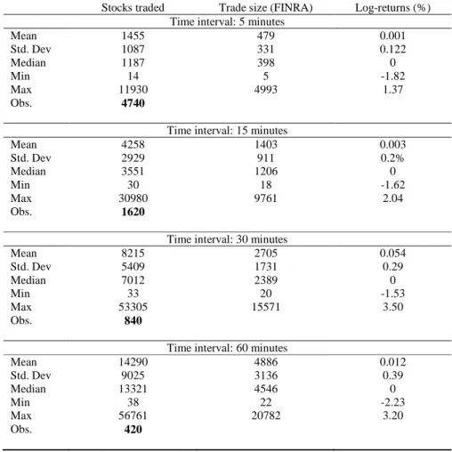
Table 1 – Summary statistics - transactions data
Stocks traded Trade size (FINRA) Log-returns (%) Time interval: 5 minutes
Mean 1455 479 0.001 Std. Dev 1087 331 0.122 Median 1187 398 0 Min 14 5 -1.82 Max 11930 4993 1.37 Obs. 4740
Time interval: 15 minutes
Mean 4258 1403 0.003 Std. Dev 2929 911 0.2% Median 3551 1206 0 Min 30 18 -1.62 Max 30980 9761 2.04 Obs. 1620
Time interval: 30 minutes
Mean 8215 2705 0.054 Std. Dev 5409 1731 0.29 Median 7012 2389 0 Min 33 20 -1.53 Max 53305 15571 3.50 Obs. 840
Time interval: 60 minutes
Mean 14290 4886 0.012 Std. Dev 9025 3136 0.39 Median 13321 4546 0 Min 38 22 -2.23 Max 56761 20782 3.20 Obs. 420
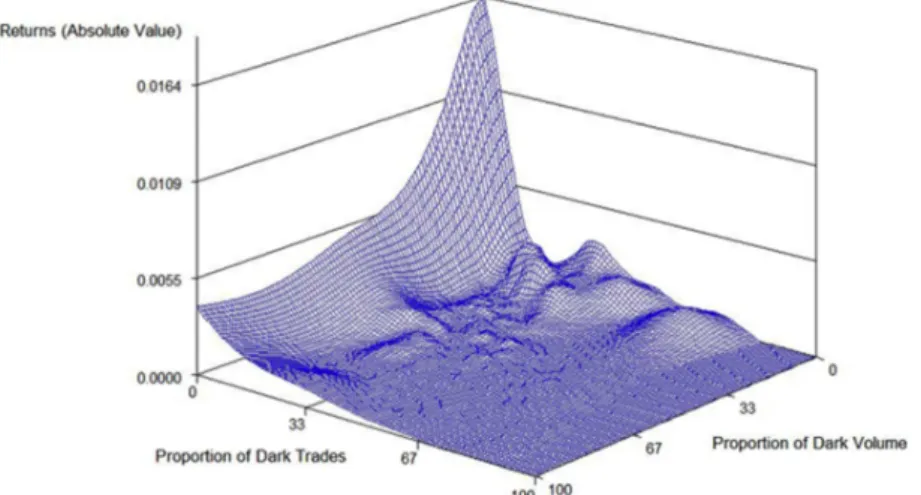
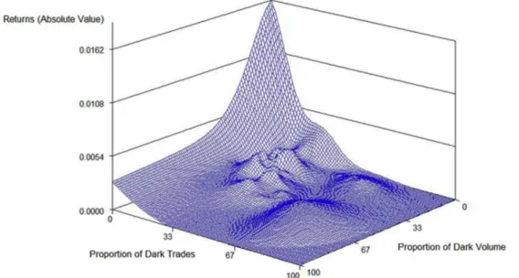
Table 1 provides summary statistics (per pre-specified time interval) for log-returns, trade size reported by other reporting trading facilities (FINRA) and all other exchanges. Then, for each pre-specified time interval; the relationship between absolute returns, proportion of dark-trades ( ) and the proportion dark volume ( ) is plotted (figures 1 – 4) in a three dimensional figure. A-priori, these figures indicate that the absolute value of log-returns decreases with respect to the proportion of dark-trades ( ) and the proportion dark volume ( ). However, a
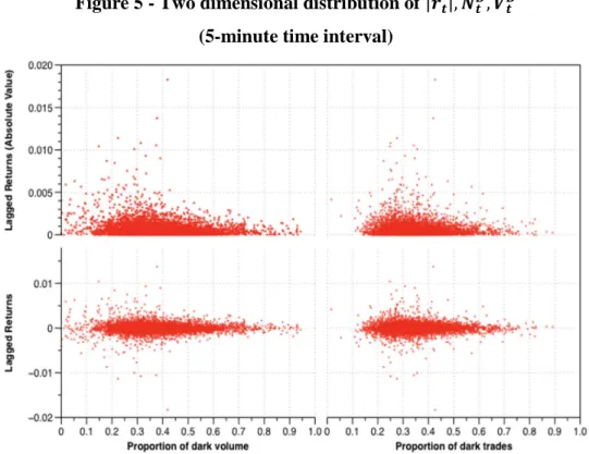
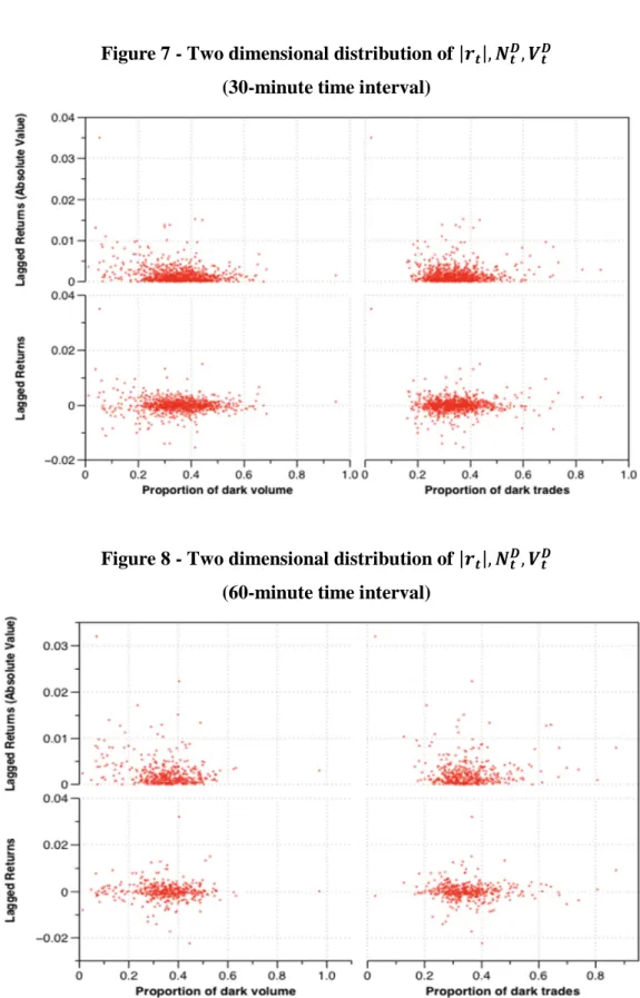
closer examination (i.e.: a two dimensional plot) reveals a concave relationship between absolute log-returns and the two proxies (proportion of dark trades and volume). Note that this concave relationship is likely to be related to dark trading occurring when volatility is low. Figures 5 – 8 plots the relationship between lead returns and lead returns absolute value with respect to and . These figures highlight the possibility of a concave relationship between dark trading and lead returns absolute value. That is, up to some threshold value dark trading activity is followed by increased returns absolute value.
Figure 1 - Distribution of | |, , (5-minute time interval)
Figure 3-Distribution of | |, , (30-minute time interval)
Figure 5 - Two dimensional distribution of | |, , (5-minute time interval)
Figure 6 - Two dimensional distribution of | |, ,
Figure 7 - Two dimensional distribution of | |, , (30-minute time interval)
Figure 8 - Two dimensional distribution of | |, ,
2. Empirical methodology
Let { } be a series of returns, and assume that the data admit the following data generating process (DGP)4: = + ! + " #ℎ ℎ%= & '+ & "% + (ℎ% + )* (3) Where:
• , &, &', & , and ( are parameters to be estimated.
• &'> 0, α > 0, ( > 0 and α + ( < 1
• ) is a (1 × 0) vector of parameters associated with the (0 × 1) matrix of exogenous variables * .
• " ∼ 3(. )
Moreover, to capture excess kurtosis in intraday returns, define 3(. ) as the Generalized Error Distribution (GED) law with 5 degrees of freedom (Nelson, 1991). We shall refer to the above model as the AR(1)-GARCHX(1,1)-GED model (‘X’ standing for included external explanatory variables), which is reduced to the AR(1)-GARCH(1,1)-GED model if ) = 0.
To analyze the informational contents of dark-trades, on the conditional variance (ht), and
then on returns, we focus on the predictive accuracy of competing AR(1)-GARCHX(1,1)-GED models, each one differing by the variables included in the matrix Xt. Especially, we focus on
pairwise comparisons based on the accuracy of out-of-sample one-step-ahead density forecasts. The use of density forecasts for comparing both nested and non-nested models is popular in economics (e.g.: Tay and Wallis, 2000). This approach bears several interesting features. First, since a density forecast is an estimate of the full one-step-ahead probability distribution function of a random variable (conditional on an information set), the comparison takes place over the full distribution (or over some regions of the distribution). Therefore, it enables us to see how dark
4
Before choosing the AR(1)-GARCH(1,1) model, we have estimated various models, also with different laws for the residuals (Student, Skew-Student, Skew-GED). Clearly the AR(1)-GARCH(1,1)-GED performs best.
trading informs us on tail events which is of main concern for the financial regulator. Second, the competing models are allowed to be only an approximation of the true underlying DGP. In other words, they are allowed to have a certain degree of misspecification. Third, tests are designed to deal with heterogeneous data. Fourth, for two nested models, the suggested approach allows to analyze the marginal influence of a given exogenous explanatory variable in terms of predictive content. Thus, providing information that is different from the one provided by the standard Student t-statistics.
Following Amisano and Giacomini (2007), define 6 = ( , *7)7 and let ℱ =σ(6 , 6%, … , 6 ) be the information set at time t. Suppose we have two competing AR(1)-GARCHX(1,1)-GED models, say : (6 , 6%, … , 6 ;< : ) ) and > ( 6 , 6%, … , 6 ?< : )%)
(where ) and )% are parameters to be estimated) and we want to rank these models according to their out-of-sample one-step-ahead forecast accuracy. We can either analyze point forecasts (e.g. Clark and McCraken, 2009) or density forecasts. Since the latter represent the complete characterization associated with the one-step-ahead forecast, it contains all the relevant information. Furthermore, let BC(. ) and BD(. ) be the two out-of-sample one-step-ahead density forecasts and let ln (BC( < )) and ln (BD( < )) be the two log-scores evaluated at the outcome
rt+1. Amisano and Giacomini (2007) suggest a test based on a loss function that uses these
logarithmic scoring rules.
Define, E ∈ (max(I, J) , ( − 1)/ ). Using a rolling scheme, one can estimate the two models on the time period 1: M = int(E ). Then, produce density forecasts and re-estimate the model on 1: M = int(E ) + 1. This procedures is repeatedly carried on, yielding two sets of n log-scores - {ln (BC( < ))} PQR(λ ) and {ln (BD( < ))} PQR(λ ). Note that by using this scheme,
we allow the models to capture structural changes in the parameters as well as in the kurtosis of the returns. To test for null of equality of density forecasts, the following statistic is used:
MS=T3U
VVVVVVVλ ,S
WX/√1 (4)
• T3UVVVVVVVλ ,S= 1 ∑ PQR(λ )T3Uλ , < ,
• T3Uλ , < = [( < ) \logBC( < ) − logBD( < )_,
• WX is an heteroskedastic and autocorrelation consistent (HAC) estimator of the standard error of T3Uλ , < over the n considered periods.
• [( < ) is a weighting function discussed below.
• < is the observed standardized returns defined as < = ( < − `̂S)/WXS, where `̂S and WXS are the unconditional mean and standard error of the n realizations of < .
Such a test is known as a Weighted Likelihood Ratio (WLR) test. Under the null, tn is
distributed as a standard Normal deviate with unit variance. Notice that a large and significant positive value for MS leads to choose f(.) over g(.). While a negative value of MS will lead to choose g(.) over f(.). The weighting function w(.) is used to set to highlight a particular region of the density forecast. If w(.) is uniform, i.e. taking the value of 1 whatever < is (case 0), then the test highlights the entire distribution. Four other definitions of w(.) are of interest for any variable y with zero mean and unit variance:
• Case 1 (Center of the distribution): [(b) = c(b), where c(. ) is the standard normal density function.
• Case 2 (Tails of distribution): [(b) = 1 − c(b)/ c(0), where c(. ) is the standard normal density function.
• Case 3 (Right tail of distribution): [(b) = Φ(b), where Φ(. ) is the standard normal distribution function.
• Case 4 (Left tail of distribution): [(b) = 1 − Φ(b), where Φ(. ) is the standard normal distribution function.
3. Empirical results and discussion
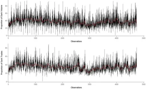
We implement the WLR test on intraday returns on Microsoft traded shares where the data is aggregated at a five-minute time interval. As mentioned above, two proxies of dark trading are used in various competing models, and . Figure 9 plots the two different measures, together with their trends estimated using a spline. Cleary, the two series exhibit similar trends, but with different volatilities.
Figure 9 – Time evolution of and (5-minute time interval)
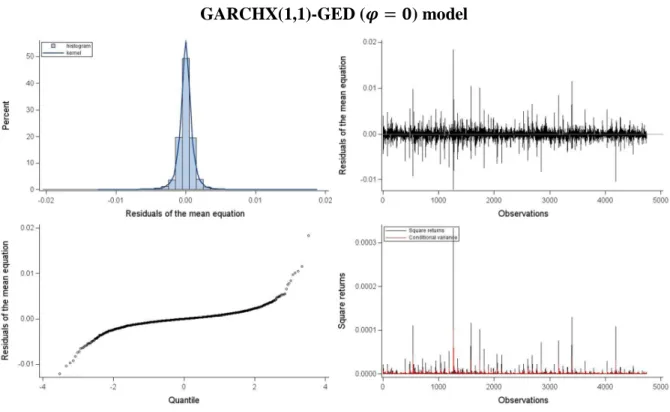
Table 2 reports the estimated parameters of the AR(1)-GARCHX(1,1)-GED model with ) = 0, which is estimated by implementing the Full Information Maximum Likelihood (FIML) framework. The autocorrelation coefficient in the mean equation is significant, and the low degree of freedom for the GED law leads to reject the normality assumption (ν = 2) in favor of a fat tailed distribution. Moreover, the model exhibits no autocorrelation (Qstat), neither heteroskedasticity (ARCH-LM) (p-values between parentheses). Figure 10 provides a panel that graphs residuals and squared returns. It indicates that the distribution of residuals seems to be symmetric, however, with high kurtosis and right tail outliers.
Table 2 – FIML Parameter estimates of the
AR(1)-GARCHX(1,1)-GED (e = f) model
Parameter Estimate Std. Err t-stat p-value -0.08669 0.0334 -2.60 0.0095
! 3.725E-9 1.776E-6 0.00 0.9983
&' 1.629E-7 2.423E-8 6.72 <.0001
& 0.279467 0.0329 8.48 <.0001 ( 0.616957 0.0377 16.35 <.0001 5 1.02131 0.0264 38.68 <.0001 Q-stat(1-6) 8.44 (0.2074) ARCH-LM (1-6) 0.92 (0.9885) VtD N t D
Figure 10 – Histogram, residuals, QQ-plots and squared returns for the
AR(1)-GARCHX(1,1)-GED (e = f) model
We next turn to pair-wise comparisons. Table 3 presents the seven competing models used in this study. The M0 one is the reference model with ) = 0, whereas models M1 to M6 all include
various proxies of dark trading. Tables 3 to 7 present the results of WLR tests. Main entries are the tn statistics and the p-values, between parentheses. A significant positive value for tn indicates
that model Mi (row) is to be preferred to Mj (column) and conversely. Clearly, four kinds of
information are of interest:
i) The information content dark trading, relative to a simple AR(1)-GARCH(1,1) model,
ii) The relative information contribution to future returns of the two proxies, i.e.: proportion of dark volume ( ) versus proportion of trades ( ).
iii) Linear versus non-linear effects of dark trading, iv) Past versus contemporaneous effects.
VtD N
t D
i. The information contribution of dark trading
We emphasize the first column of tables 3 to 7 with a special attention on models M1 and
M3 (rows 2 and 4). The indicate that these models over-perform the simple (or, benchmark)
AR(1)-GARCH(1,1)-GED model (M0 ) in terms of one-step-ahead density forecast (case 0).
Nevertheless, these two models do not provide the same information regarding returns on one-step-ahead forecast. For instance, using as an explanatory variable does not significantly improve the forecasting performances over the simple AR(1)-GARCH (1,1) model when only the center of the distribution is considered (table 4). However, it returns important information about right and left tails (Table 5). For regulators, evaluating the possible uncertainty associated with dark trading, it is an important result. Conversely, including does improve forecasts for both the center of the distribution and for the tails. In other words including or in the variance equation yields significant information about the likelihood of extreme intraday movements in the price of traded shares.
Table 3 – Estimated models
Model Mean Equation
Variance Equation
GARCH (p,q) Exogenous Variables Distribution of Errors
g' AR(1) p=1,q=1 None GED
g AR(1) p=1,q=1 GED g% AR(1) p=1,q=1 , ( )% GED gh AR(1) p=1,q=1 GED gi AR(1) p=1,q=1 , ( )% GED gj AR(1) p=1,q=1 GED gk AR(1) p=1,q=1 , ( )% GED
Table 4 - Weighted Likelihood Ratio tests Case 0 – (the entire distribution), λλλλ=0.75.
Model g' g g% gh gi gj gk g' g 3.956 (0) g% 3.487 (0) 2.840 (0.004) gh 5.851 (0) 0.169 (0.865) -1.942 (0.05) gi 4.962 (0) 4.190 (0) 1.817 (0.069) 4.224 (0) gj 2.274 (0.022) -2.167 (0.03) -2.947 (0.00) -2.476 (0.03) -4.373 (0) gk 2.343 (0.019) -1.395 (0.16) -2.989 (0.00) -1.391 (0.16) -4.258 (0) 0.458 (0.646)
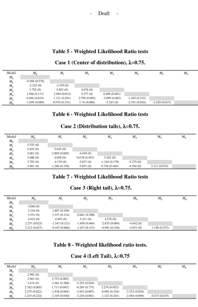
Table 5 - Weighted Likelihood Ratio tests Case 1 (Center of distribution), λλλλ=0.75.
Model g' g g% gh gi gj gk g' g -0.568 (0.570) g% -2.242 (0) -3.329 (0) gh 3.792 (0) 5.852 (0) 4.676 (0) gi 1.566 (0.117) 2.494 (0.012) 5.377 (0) 0.409 (0.681) gj 0.496 (0.619) 1.121 (0.261) 2.799 (0.005) -3.099 (0.002) -1.462 (0.143) gk -1.699 (0.089) -0.970 (0.331) 1.74 (0.080) -5.243 (0) -2.391 (0.016) -2.429 (0.015)
Table 6 - Weighted Likelihood Ratio tests Case 2 (Distribution tails), λλλλ=0.75.
Model g' g g% gh gi gj gk g' g 5.525 (0) g% 5.825 (0) 5.645 (0) gh 5.601 (0) -2.805 (0.005) -4.949 (0) gi 5.688 (0) 4.059 (0) -0.678 (0.497) 5.362 (0) gj 3.782 (0) -4.139 (0) -5.837 (0) -1.344 (0.178) -5.279 (0) gk 3.481 (0) -1.286 (0.198) -5.851 (0) 0.756 (0.449) -4.394 (0) 2.111 (0.034)
Table 7 - Weighted Likelihood Ratio tests Case 3 (Right tail), λλλλ=0.75.
Model g' g g% gh gi gj gk g' g 3.046 (0) g% 2.318 (0) 1.607 (0.108) gh 5.551 (0) 1.537 (0.124) -0.661 (0.508) gi 4.915 (0) 4.992 (0) 3.311 (0) 4.276 (0) gj 2.237 (0.025) -1.547 (0.121) -1.850 (0.064) -2.835 (0.004) -4.642 (0) gk 2.212 (0.027) -0.167 (0.866) -1.427 (0.153) -0.981 (0.326) -4.051 (0) 1.140 (0.253)
Table 8 - Weighted likelihood ratio tests. Case 4 (Left Tail), λλλλ=0.75
Model g' g g% gh gi gj gk g' g 2.982 (0) g% 2.961 (0) 2.753 (0.005) gh 3.474 (0) -1.061 (0.288) -2.255 (0.024) gi 2.762 (0.005) 1.713 (0.087) -0.285 (0.775) 2.276 (0.022) gj 2.275 (0.022) -1.838 (0.065) -2.653 (0.007) -0.985 (0.324) -2.252 (0.024) gk 1.215 (0.224) -2.165 (0.030) -3.254 (0.001) -1.122 (0.261) -2.584 (0.009) -0.473 (0.635)
ii. Proportion of dark volume vs. proportion of dark trades
Including or in the variance equation provides different information when examining their effects on the center of the distribution. Nevertheless, these models significantly over-perform the benchmark model (M0) in analyzing distribution tails. Emphasizing the second
column in table 4 (case 0) the two models appear to be equivalent. However, tables 5 and 6 reveal a slightly different reality, i.e.: model M3 is over performs model M1 when only the center
of the distribution is considered. This result is consistent with the results reported earlier. Moreover, table 6 indicates that model M1 should be chosen when forecasts of the distribution
tails are being emphasized. To summarize, the two proxies provide different information about future returns realizations. However, the proportion of dark-trades ( ) seem to provide superior information regarding the one-step-ahead density.
iii. Linear vs. non-linear effects
Previously we have indicated that there might be a non-linear effects of dark trading on returns variance (Figures 1 and 8). To examine this possibility, we perform a pairwise comparison of model M2 relative to M1 and of model M4 relative to M3. With regard to the former
comparison, results are of a particular interest: M2 over-performs M1 (case 0). This result
appears to be due to its ability to forecast the tails of the returns, especially the left tail (that corresponds to losses). Thus, it provides crucial information concerning the Value at Risk (VaR) metric. For the center of the distribution, M1 still over-performs model M2.
A similar pattern appears in latter comparison since M4 over-performs M3. Especially
when considering the tails (right and left). If we compare M4 relative to M2, it seems that the
former performs better while considering the center of the distribution. This is also the case when considering the right tail of the distribution. Therefore, the proportion of dark trades ( ) provides superior information while considering non-linear relationships with returns.
VtD NtD
iv. Past vs. contemporaneous effects
At last, we analyze whether including past information about contributes significant information in volatility equation. By comparing models M5 and M6 to M4, it appears the latter
performs best. This is valid for all considered case (the entire or only section of the distribution). This result is rather surprising (as well as all previously discussed results) because the proportion of dark volume includes information on contemporary and past transactions price. Though not investigated here, it seems that these results provide evidence that intraday price is a martingale.
4. Conclusion
In this paper we have applied the GARCH estimation framework to a problem of market microstructure. More precisely, we have attempted to answer whether the activity of trading in the dark (trading in dark-pools) conveys any information on the intraday return and volatility process. Our results indicate that indeed dark trading activity conveys relevant information to the process determining one-step-ahead returns. Moreover, not only it conveys information over the one-step-ahead return forecast, it also conveys important information on the entire density forecast of returns. This, with a special emphasis on the tails of this density forecast. Hence, we conclude that dark-trading has an important role in determining intraday returns and the uncertainty that may relate to them.
Furthermore, our results indicate that number of dark trades within a predetermined time-interval provides more information regarding the (one-step-ahead) point and density forecast of returns. Moreover, for non-linear relationships that affect the volatility process, the proportion of dark trades also provides more information. Though we do not discuss the issue of price discovery, it is obvious that dark trading has a role in the price discovery process. From our results, it seems that it may contribute to the price discovery process in the case of Microsoft stock.
Given highlighted results, dark trading may provide valuable information to regulators and market participants alike. For regulators, dark trading maybe provide information over the
effects of high - frequency trading, provided that dark trading activity coincides with the latter activity. Therefore, an important issue for further research is to empirically determine how trading in the dark coincides with high frequency trading. Determining this relationship may provide an important piece of information for regulators in the activity of overseeing financial markets. Another important outcome of the indicated results is that dark-trading seems to be well integrated in current trading activity. Furthermore, as mentioned already, it seems that traders on public exchanges react to dark trading once it is exposed to the public.
Besides determining the relationship between high-frequency (or more generally, informed trading) and dark trading, further research will require to expand our stocks universe to include more stocks with different trading characteristics as well as different time periods. That is: we pre-assume that dark trading activity had a different few years ago. Thus it is necessary to analyze how dark-pool trading played role in the last ten or more years.
References
Amisano, G., & Giacomini, R. (2007). Comparing density forecasts via weighted likelihood ratio tests. Journal of Business & Economic Statistics,25(2), 177-190.
Bessembinder, H., Panayides, M., & Venkataraman, K. (2009). Hidden liquidity: an analysis of order exposure strategies in electronic stock markets.Journal of Financial Economics, 94(3), 361-383.
Boni, L., Brown, D., & Leach, J. (2012). Dark Pool Exclusivity Matters.Available at SSRN
2055808.
Buti, S., Rindi, B., & Werner, I. (2011). Diving into Dark Pools. Charles A. Dice Center
Working Paper, (2010-10).
Clark, T. E., & McCracken, M. W. (2009). Tests of equal predictive ability with real-time data. Journal of Business & Economic Statistics, 27(4), 441-454.
Kratz, P., & Schöneborn, T. (2012, April). Optimal liquidation in dark pools. In EFA 2009
Bergen Meetings Paper.
Nelson, D. B. (1991). Conditional heteroskedasticity in asset returns: A new approach. Econometrica: Journal of the Econometric Society, 347-370.
Nimalendran, M., & Ray, S. (2011). Informed trading in dark pools. Working paper University of Florida.
Nimalendran, M., & Ray, S. (2013). Informational linkages between dark and lit trading venues. Journal of Financial Markets.
O'Hara, M., & Ye, M. (2011). Is market fragmentation harming market quality?.Journal of
Financial Economics, 100(3), 459-474.
Ready, M. (2009, December). Determinants of volume in dark pools. In AFA 2010 Atlanta
Meetings Paper.
Tay, A. S., & Wallis, K. F. (2002). Density forecasting: a survey. Companion to Economic
Forecasting, 45-68.
Weaver, D. (2011). Internalization and market quality in a fragmented market structure. Available at SSRN 1846470.
Ye, M. (2010). A Glimpse into the Dark: Price Formation, Transaction Cost and Market Share of the Crossing Network. Transaction Cost and Market Share of the Crossing Network (June 9,
2011).