HAL Id: hal-01207165
https://hal.inria.fr/hal-01207165
Submitted on 28 Apr 2016
HAL is a multi-disciplinary open access
archive for the deposit and dissemination of
sci-entific research documents, whether they are
pub-lished or not. The documents may come from
teaching and research institutions in France or
abroad, or from public or private research centers.
L’archive ouverte pluridisciplinaire HAL, est
destinée au dépôt et à la diffusion de documents
scientifiques de niveau recherche, publiés ou non,
émanant des établissements d’enseignement et de
recherche français ou étrangers, des laboratoires
publics ou privés.
Distributed under a Creative Commons Attribution| 4.0 International License
MEM-diffusion MRI framework to solve MEEG inverse
problem
Brahim Belaoucha, Jean-Marc Lina, Maureen Clerc, Théodore Papadopoulo
To cite this version:
Brahim Belaoucha, Jean-Marc Lina, Maureen Clerc, Théodore Papadopoulo. MEM-diffusion MRI
framework to solve MEEG inverse problem. 2015 23rd European Signal Processing Conference
(EU-SIPCO), Aug 2015, Nice, France. �hal-01207165�
MEM-diffusion MRI framework to solve MEEG inverse problem
Brahim Belaoucha
†,‡Jean-Marc Lina
?,??Maureen Clerc
†Th´eodore Papadopoulo
††
Athena Project-Team, Inria Sophia Antipolis-M´editerran´ee, France
‡
Universit´e Cˆote d’Azur, Nice, France
?
Centre de Recherches Math´ematique, Montr´eal, Canada
??
D´epartement de G´enie Electrique, ETS, Montr´eal, Canada
ABSTRACT
In this paper, we present a framework to fuse information coming from diffusion magnetic resonance imaging (dMRI) with Magnetoencephalography (MEG)/ Electroencephalogra-phy (EEG) measurements to reconstruct the activation on the cortical surface. The MEG/EEG inverse-problem is solved by the Maximum Entropy on the Mean (MEM) principle and by assuming that the sources inside each cortical region follow Normal distribution. These regions are obtained using dMRI and assumed to be functionally independent. The source re-construction framework presented in this work is tested using synthetic and real data. The activated regions for the real data is consistent with the literature about the face recognition and processing network.
Index Terms— MEG, EEG, dMRI, source reconstruc-tion, parcellareconstruc-tion, MEM.
1. INTRODUCTION
Magneto and electroencephalography (MEEG) are non-invasive modalities which provide an insight on the temporal succession of cognitive processes. Finding the activation is an underdetermined problem due to the large number of un-knowns i.e. dipoles (distributed sources) with compared to the number of measurements. A solution is obtained by as-suming a prior on the solution. Different prior choices of lead to different approaches [1]. They can be divided into two cat-egories: linear and nonlinear approaches. Linear approaches overestimate the sources’ intensities. Nonlinear approaches, like MEM, do not suffer from this limitation.
Physiologically, the brain is organized in functional ar-eas [2]. In the previous MEM source estimation papers, functional imaging (fMRI) and the Multivariate Source Pre-localization (MSP) [3] have been used to parcellate the corti-cal surface. However, these approaches give different parcel-lations per subject depending on the functional data. dMRI is a non-invasive imaging modality which gives the diffusion of water in the tissues, as a result it reveals the fiber structure. In this work, we define a unique cortical parcellation for each subject that depends only on the brain anatomy. We use dMRI
information to segment the white/gray (W/G) matter interface into some correlate of functional areas as in Anwander et al. [4], but we extend this approach to work on the whole cor-tex. We then integrate the cortical surface parcellation in the MEM framework [5] presented in section 2. The sources in-side each region are assumed to follow a Normal distribution, and for simplicity we consider them functionally indepen-dent. We evaluate the accuracy of the source estimates using synthetic and real MEEG measurements obtained from a face recognition task. The resulting active regions of the MEM-dMRI approach is compared to the Minimum norm estimate (MNE) [1] and what can be found in literature about face processing and recognition network.
2. MEM-DMRI FRAMEWORK
2.1. MEM
For each task, let M ∈ RC×N ×T (C number of sensors, N number of task repetitions, T the time window length) denote the measurements, (magnetic field for MEG, electrode poten-tial for EEG). R ∈ RSr×N ×T (Sr number of sources) be the source intensities, and G ∈ RC×Sr be the lead field matrix. m ∈ RC×T is the averaged signal over repetitions of M i.e.
m = E[M ] and can be written as: m = GE[R] + ε
where ε is a zero mean Gaussian measurement noise. The MEM framework maximizes the information coming from the measurements, by maximizing the entropy of the mean signal. Let’s assume that the dipole intensities follow the probability law; p(r) = f (r)µ(r), where µ is the refer-ence probability distribution of all dipoles (denoted by r) in the cortical surface without any MEG/EEG measurements. Let’s consider the Kullback-Leibler’s pseudo-distance be-tween the reference and the real distribution of the dipoles intensities [5]
Sµ(p) = −
Z
p log p
µ (1)
The probability law, p, is chosen to maximize the information brought by the measurements. This yields to the definition of
the following objective function L to be minimized:
L(p, λ, λ0) = −Sµ(p) + λt(m − Gr) + λ0(1 −
Z
p) (2) where (.t) denotes the transpose. The dipole intensity is given by [5]:
˜
r = ∇Fµ(X)|X=Gt˜λ (3)
where Fµis the log of the partition function associated to the
distribution µ
Fµ(Gtλ) = log
Z
exp(λtGr)µ(r)
and ˜λ is the vector defined by; ˜
λ = argmaxλ(λ tm − F
µ) (4)
In the presence of noise with the probability measure dµn,
equation (4) is still valid, we need just to replace Fµ(Gtλ) by˜
Fµ(Gtλ) + F˜ dµn(˜λ) [5].
2.2. MEM-dMRI
fMRI and MSP were used to parcellate the cortical surface and used in the MEM framework. They give different parcel-lations per subject depending on the functional data. In this paper, we use dMRI to parcellate (see section 3.1) the corti-cal surface into K corticorti-cal parcels,{P1, .., PK}. The sources
in each region are assumed to follow a Normal distribution. Each parcel has two possible states, i.e. for a region i, Si ∈
{0, 1}, which represents inactive and active regions respec-tively. Using this information, the reference probability for independent regions can be found as explained in [5]:
µ(r) = K Y k=1 1 X Sk=0 π(Sk)µ(rk|Sk) (5)
where π is the joint probability law of Skand rkis the sources
inside the kthregion. Using this definition and (3), the MEM
estimate is [5]: ˜ ri,k= X S ˜ π(S)∇iFSk(X)|X=Gt k˜λ (6) where ∇iFSk(X)|X=Gt
kλ˜ is the estimation of ri, a dipole i
in the parcel Pk for a given state Sk, the summation over S
runs over all the configuration of S = {S1, S2, .., Sk}, Gkis a
submatrix of G that contains the contribution of only sources in region Pk, and FSk represents the log-partition function
associated to the region k, and is defined as:
FSk(G t k˜λ) = log Z exp(λtGkrk)µ(rk|Sk) ˜ π(S) = QK k=1π(S˜ k) exp FSk(G t kλ)˜ P S QK k=1π(S˜ k) exp FSk(G t k˜λ)
For independent regions, the posterior conditional probability equals: ˜ π(Sk) = π(Sk) exp FSk(G t kλ)˜ P Skπ(Sk) exp FSk(G t k˜λ) (7)
The joint reference law is considered as:
µ(rk|Sk= 0) = δ(rk)
µ(rk|Sk= 1) = N (νk, Σk)
(8)
where δ refers to the Dirac function, and N (νk, Σk) is a
Gaus-sian distribution that explains the dipole’s intensities inside an active patch. Let’s αkbe the probability of the region Pkto be
active, i.e. π(Sk = 1) = αk. We chose zero mean (νk = 0)
and a covariance matrix (Σk) like in Chowdhury et al. [3] and
Friston et al. [6]. The α0s are initialized using the mean of the multivariate source pre-localization [7] scores inside the parcels obtained by the dMRI parcellation and is then updated using (7).
3. IMAGE ACQUISITION AND PROCESSING
Structural and diffusion MRI data were taken from 11 healthy subjects [8, 9]. The T1 weighted images of size 256 × 256 × 192 were acquired by Siemens 3T Trio with GRAPPA 3D MPRAGE sequence (TR = 2250 ms; TE = 2.99 ms; flip-angle = 9 degree; acceleration factor = 2) at 1 mm isotropic reso-lution. The diffusion weighted images of size 96 × 96 × 68 were collected by the same scanner at 2 mm isotropic resolu-tion (64 gradient direcresolu-tions and b-value =1000 s/mm2) , with one b0 image.
The W/G matter interfaces were extracted using Freesurfer [10] from T1 and remeshed to 104 vertices using
Brain-storm [11], then projected from the anatomical to the dif-fusion space. The projection was obtained by registering the brain in the two spaces using FSL [12]. The MEG/EEG forward problem, based on Boundary Element Method, is ob-tained using OpenMEEG [13] with a brain-skull conductivity ratio set to 80.
MEG and EEG were measured in magnetically shielded room using Elekta Neuromag Vectorview 306 system (102 magnetometers, 204 planar gradiometers), a 70 easy channel Easycap EEG cap was used to record the EEG data simultane-ously. Stimuli were presented in six 7.5 min runs at 1100 Hz sampling rate. The face stimuli contains two sets of 300 gray-scale photographs, half from unfamiliar people (unknown to the subjects) and the remaining from famous people. For the third condition, 150 photographs of scrambled faces are ob-tained from either famous or unfamiliar people.
Across subjects, between 880 and 889 epochs were ex-tracted (around 295 per condition i.e. Famous (Fs), Unfamil-iar (Ur), Scrambled (Sd)) [8, 9]. For each of the 11 partici-pants and conditions, we averaged the EEG and MEG mea-surements. This allows us to increase the signal-to-noise ratio
Fig. 1: The cross-correlation matrix (CM) between all the connec-tivity profiles of the sources in the left ST lobe. A column or raw i (symetric matrix) corresponds to the correlation between the con-nectivity profile of source i and all the others in the pre-parcel.
and have an average overview on the cortical regions respon-sible of the face recognition. More details of the paradigm can be found on [9]. Low-pass filter from MNE-Python pack-age [14] with a cutoff frequency equal to 45 Hz was used. Due to the page limitation, we show the results of only 4 subjects (2 male, 2 female, mean age 26.75).
3.1. Cortex parcellation
Due to the speed and memory limitations caused by the high number of sources (104), we use pre-parcellated cortical sur-face as an initial parcellation. We use the same approach as described in Anwander et al. [4], but instead of using Brod-mann atlas as a pre-parcellation, we use Destrieux atlas pro-vided by FreeSurfer. For each Destrieux region, we compute the connectivity profiles (tractograms) of the cortical sources (seeds).
The connectivity profile of a seed i, a vector of size D, is the connectivity strength, i.e. the number of samples drawn from i that arrives to a voxel j, between seed i and all of the other voxels in the image space. It represents the distribution of the fibers that starts from i. It is obtained via a probabilis-tic tractography using FDT [15] toolbox from FSL. We define
Fig. 2: The resulting parcellation of Subject 1 with Cth= 65.
dMRI patch as a region in which sources have similar con-nectivity profiles. We apply k-means on the cross-correlation matrix (CM) to parcellate each of the pre-parcels. The num-ber of regions (clusters), ni, inside the ithpre-parcels is
cho-sen so that the ni first biggest eigenvalues of CM represent
more than a threshold Cth(in %) of the total energy of CM.
P P P P P P PP Cth Subject 1 2 3 4 60 308 297 295 304 70 431 400 415 432 80 503 544 537 533
Table 1: The total number of regions for different subjects and Cth
values. Close numbers across subjects.
This approach does not guarantee the regions to be spatially connected. Fig. 1 shows the correlation between pairs of con-nectivity profiles inside the left Superior Temporal (ST) lobe, ST can be divided into sub-regions with similar connectivity profiles. We follow the same procedure with the rest of the pre-parcels. Table 1 shows the resulting number of parcels for four different subjects and different threshold values. As expected, the number increases with the threshold value, for Cth= 100 every region contains only one source.
4. RESULTS AND DISCUSSION
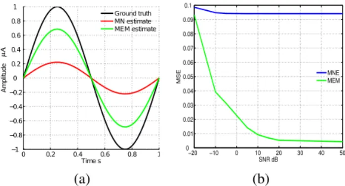
Fig. 3 (a) compares the source reconstruction of the MEM and Minimum norm estimate (MNE) [1] on synthetic data in which one region in the Precentral gyrus (2.47 cm2) was acti-vated. The ground truth is a sine wave. In Fig. 3 (b), we show the effect of an additive Gaussian noise on the source recon-struction of both approaches by computing the mean squared error (MSE) between the ground truth and the estimates.
0 0.2 0.4 0.6 0.8 1 −1 −0.8 −0.6 −0.4 −0.2 0 0.2 0.4 0.6 0.8 1 Time s A m pl itu de Ground truth MN estimate MEM estimate µ A (a) −20 −10 0 10 20 30 40 50 0 0.01 0.02 0.03 0.04 0.05 0.06 0.07 0.08 0.09 0.1 SNR dB MSE MNE MEM (b)
Fig. 3: Results of synthetic data, (a) the source reconstruction us-ing MNE (red) and MEM (green) and (b) the MSE versus SNR for both MNE (blue) and MEM (green). MNE gives an average error of around 10% whereas MEM decreases until less than 0.5% error.
The MEM provides more accurate results and is less af-fected by noise than the MN estimate. The regularization in MNE is the l2norm on the source (the trade off parameter is
fixed by the Generalized Cross Validation ). This smooths the intensities which reduces the reconstructed values.
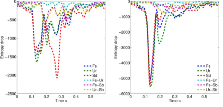
The framework is tested now using the real data presented in section 3. Cthis set to 70 for all subject. Fig. 4 shows
the entropy drop, equation (1), over time for 2 subjects and different conditions. Fs-Ur represents the measurements ob-tained for famous photographs subtracted to the ones obob-tained
(a) Subject 1 (b) Subject 2
Fig. 4: Entropy drop due to the MEG measurements of different classes and subjects. The decrease in the entropy drop for the Fs, Ur, Sd starts around 70 ms.
for unfamiliar photographs, the same for Fs-Sd, and Ur-Sd. The entropy curves starts significantly decreasing at around 70 ms which coincide with the literature about the visually evoked potential time. The entropy drop of Fs-Ur measure-ments is smaller than the other classes which means that the information brought by the MEG measurements was reduced by subtracting the measurements of Fs to Ur. Fig.5 shows the averaged absolute dipoles intensities (AADI) for Fs-Sd of the different subjects between 60 ms and 400 ms after the stimu-lus.
AADI =
P400 ms
t = 60msabs(rt)
number of time samples
This measure gives us the average activation of dipoles over the time window of interest and give us an insight about which cortical regions are activated during face recognition task.
Sources in Fig.5 (c) and (d) are obtained using the Min-imum Norm estimate [1] on MEG and EEG measurements respectively. The MEM-dMRI framework is used to recon-struct sources intensity from the MEG (Fig.5 (a)) and EEG measurements (Fig.5 (b)) of 4 subjects. MNE smooths the sources over the cortex which make it hard to find the real activated regions, whereas MEM provided a focal solution. The later solution is consistent with previous studies and re-sults concerning face recognition network as shown in [16], and also to the fMRI and MEG source reconstruction of the same data set in Henson et al. [8] but with different source re-construction algorithm in which the Inferior Occipital Gyrus (IOG) and the Fusiform gyrus (FFG) region (see Fig. 5 (e)) were found to be active. Some studies reported bilateral acti-vation [17, 18], Subject 1-3. Others reported right sided pre-frontal activation [19], see the EEG reconstruction of Subject 4 (panel 4 in Fig. 5 (b)).
Although both MEG and EEG measures the same neuro-physiological processes, they are different. MEG is less af-fected by Skull and Scalp than EEG. The latter is sensitive to the tangential and radial sources, whereas MEG is sensitive to tangential sources. These lead to differences in the recon-struction between the MEG (Fig. 5 (a)) and EEG (Fig. 5 (b)).
(a) (b)
(c) (d)
(e) (f)
Fig. 5: Averaged absolute dipoles intensities estimated by: (a) MEM on MEG, (b) MEM on EEG, (c) MNE on MEG, (d) MNE on EEG for different subjects. All values were normalized to be between 0 and 1. Numbers 1-4 represents the subject number , (e) location of IOG in orange and FFG in blue in the cortex. (f) the different views in each box.
5. CONCLUSION
This paper presents a way to fuse a high spatial resolution imaging (dMRI) information to the MEM framework. This allows us to define one parcellation per subject and to use the focality advantage of the MEM. This is useful to compare the activated regions between different tasks and for multi-subject studies. Sources inside each region obtained from the dMRI informed parcellisation of the cortical substrate are assumed to follow Normal distribution and functionally independent. Synthetic and real data were used to test the reconstruction algorithm and compared with the reconstruction of MNE. For real MEG/EEG data, the results of the framework was found to be consistent with what we can find in the literature about face recognition task. For future work, MEM-dMRI will be used for functionally dependent regions case. The effect of adding a temporal regularization should be investigated.
6. ACKNOWLEDGMENT
We acknowledge Alexandre Gramfort for providing the code used for EEG/MEG pre-processing.
REFERENCES
[1] R. Grech, T. Cassar, et al., “Review on solving the in-verse problem in eeg source analysis,” Journal of Neu-roEngineering and Rehabilitation, vol. 5, no. 1, pp. 25, 2008.
[2] B. Cottereau, K. Jerbi, et al., “Multiresolution imag-ing of MEG cortical sources usimag-ing an explicit piecewise model,” NeuroImage, vol. 38, no. 3, pp. 439 – 451, 2007.
[3] R. A. Chowdhury, J. M. Lina, et al., “MEG source lo-calization of spatially extended generators of epileptic activity: Comparing entropic and hierarchical bayesian approaches,” PLoS ONE, vol. 8, no. 2, pp. e55969, 2013.
[4] A. Anwander, M. Tittgemeyer, et al., “Connectivity-based parcellation of Broca’s area,” Cerebral Cortex, vol. 17, no. 4, pp. 816–825, 2007.
[5] C. Amblard, E. Lapalme, et al., “Biomagnetic source detection by maximum entropy and graphical models,” Biomedical Engineering, IEEE Transactions on, vol. 51, no. 3, pp. 427–442, 2004.
[6] K. Friston, L Harrison, et al., “Multiple sparse priors for the M/EEG inverse problem,” NeuroImage, vol. 39, no. 3, pp. 1104–1120, 2008.
[7] J. Mattout, M. P´el´egrini-Issac, et al., “Multivariate source prelocalization (MSP): Use of functionally in-formed basis functions for better conditioning the MEG inverse problem,” NeuroImage, vol. 26, no. 2, pp. 356 – 373, 2005.
[8] R. N. Henson, D. G. Wakeman, et al., “A parametric Empirical Bayesian framework for the EEG/MEG in-verse problem: generative models for multisubject and multimodal integration,” Frontiers in Human Neuro-science, vol. 5, no. 76, 2011.
[9] D. G. Wakeman and R. N. Henson, “A multi-subject, multi-modal human neuroimaging dataset,” Scientific Data, 2015.
[10] A.M. Dale, B. Fischl, et al., “Cortical surface-based analysis I: Segmentation and surface reconstruction,” NeuroImage, vol. 9, pp. 179194, 1999.
[11] F. Tadel, S. Baillet, et al., “Brainstorm: A user-friendly application for MEG/EEG analysis,” Computational In-telligence and Neuroscience, vol. 2011, no. 1, pp. 19, 2011.
[12] S. M. Smith, M. Jenkinson, et al., “Advances in func-tional and structural MR image analysis and implemen-tation as FSL,” NeuroImage, vol. 23, Supplement 1, no. 0, pp. S208 – S219, 2004, Mathematics in Brain Imag-ing.
[13] A. Gramfort, T. Papadopoulo, et al., “OpenMEEG: opensource software for quasistatic bioelectromagnet-ics,” BioMedical Engineering OnLine, vol. 9, no. 1, pp. 45, 2010.
[14] A. Gramfort, M. Luessi, et al., “MEG and EEG data analysis with mne-python,” Frontiers in Neuroscience, vol. 7, no. 267, 2013.
[15] T.E.J. Behrens, H. Johansen Berg, et al., “Probabilistic diffusion tractography with multiple fibre orientations: What can we gain?,” NeuroImage, vol. 34, no. 1, pp. 144 – 155, 2007.
[16] B. Rossion, R. Caldara, et al., “A network of occipito-temporal face-sensitive areas besides the right middle fusiform gyrus is necessary for normal face process-ing,” Brain, vol. 126, no. 11, pp. 2381–2395, 2003. [17] A. Ishai and E. Yago, “Recognition memory of newly
learned faces,” Brain Research Bulletin, vol. 71, no. 13, pp. 167 – 173, 2006.
[18] J.V. Haxby, L.G. Ungerleider, et al., “The effect of face inversion on activity in human neural systems for face and object perception,” Neuron, vol. 22, no. 1, pp. 189 – 199, 1999.
[19] D.J. Bayle and M.J. Taylor, “Attention inhibition of early cortical activation to fearful faces,” Brain Re-search, vol. 1313, no. 0, pp. 113 – 123, 2010.