HAL Id: halshs-00564934
https://halshs.archives-ouvertes.fr/halshs-00564934
Preprint submitted on 10 Feb 2011
HAL is a multi-disciplinary open access
archive for the deposit and dissemination of sci-entific research documents, whether they are pub-lished or not. The documents may come from teaching and research institutions in France or
L’archive ouverte pluridisciplinaire HAL, est destinée au dépôt et à la diffusion de documents scientifiques de niveau recherche, publiés ou non, émanant des établissements d’enseignement et de recherche français ou étrangers, des laboratoires
Compensating the dead? Yes we can!
Marc Fleurbaey, Marie-Louise Leroux, Grégory Ponthière
To cite this version:
Marc Fleurbaey, Marie-Louise Leroux, Grégory Ponthière. Compensating the dead? Yes we can!. 2010. �halshs-00564934�
WORKING PAPER N° 2010 - 34
Compensating the dead?
Yes we can!
Marc Fleurbaey Marie-Louise Leroux
Grégory Ponthière
JEL Codes: D63, D71, I18, J18
Keywords: compensation, longevity, mortality, fairness, redistribution
P
ARIS-
JOURDANS
CIENCESE
CONOMIQUES48,BD JOURDAN –E.N.S.–75014PARIS TÉL. :33(0)143136300 – FAX :33(0)143136310
www.pse.ens.fr
Compensating The Dead?
Yes We Can!
Marc Fleurbaey
y, Marie-Louise Leroux
zand Gregory Ponthiere
xOctober 20, 2010
Abstract
An early death is, undoubtedly, a serious disadvantage. However, the com-pensation of short-lived individuals has remained so far largely unexplored, probably because it appears infeasible. Indeed, short-lived agents can hardly be identi…ed ex ante, and cannot be compensated ex post. We argue that, de-spite the above di¢ culties, a compensation can be carried out by encouraging early consumption in the life cycle. In a model with heterogeneous preferences and longevities, we show how a speci…c social criterion can be derived from intuitive principles, and we study the corresponding optimal policy under var-ious informational assumptions. We also study the robustness of our solution to alternative types of preferences and savings policies.
Keywords: compensation, longevity, mortality, fairness, redistribution. JEL codes: D63, D71, I18, J18.
The authors thank François Maniquet, Pierre Pestieau, Giacomo Valletta and Stéphane Zuber for helpful discussions on this paper.
yCNRS, University Paris-Descartes, CORE, Sciences Po, LSE, IDEP. zCORE, Université catholique de Louvain.
xEcole Normale Supérieure, Paris School of Economics [corresponding author]. Contact:
ENS, Bd Jourdan, 48, building B, second ‡oor, o¢ ce B., 75014 Paris (France). E-mail: [email protected]
1
Introduction
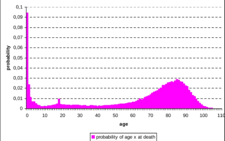
It is undeniably true that an early death constitutes a serious loss, even when it is due to natural causes. Such a loss should, in a fair society, imply a compensation. However, the compensation of short-lived persons has remained so far largely un-explored in policy circles. The absence of debate on that issue is surprising, since longevity inequalities are widely documented. It is well-known that sizeable longevity
di¤erentials exist even within a given cohort, as shown by Figure 1.1 Although all
cohort members are, by de…nition, born in the same country and at the same epoch, there is a substantial dispersion of the age at death, some persons turning out to have longer lives than others.
0 0,01 0,02 0,03 0,04 0,05 0,06 0,07 0,08 0,09 0,1 0 10 20 30 40 50 60 70 80 90 100 110 age pr oba bi li ty
probability of age x at death
Figure 1: Distribution of the age at death: Swedish female (1900 cohort)
Given that longevity di¤erentials are mainly explained by factors on which indi-viduals have, on their own, little control, there exists a strong ethical intuition for compensating short-lived agents, who are, in some sense, victims of the arbitrariness of Nature.2 Longevity inequalities due to di¤erences in genetic backgrounds are the
best illustration of this. According to Christensen et al (2006), about one quarter to one third of longevity inequalities within a cohort can be explained by di¤erences in
1Sources: the Human Mortality Data Base (2009).
2Note that longevity is also in‡uenced by individuals, for instance through their lifestyles (see
Kaplan et al 1987), but those behavioural determinants of longevity (e.g. smoking, diet, physical activity, etc.) only explain one part of longevity di¤erentials, the rest remaining out of individuals’ control (e.g. genetic background, environmental determinants of longevity, etc.).
the genetic background. Hence there is a strong intuitive support for compensating the short-lived, who cannot be regarded as responsible for their genes.
But despite the sizeable — and largely arbitrary — longevity di¤erentials, little attention has been paid to the compensation of short-lived agents. The reason behind that neglect lies in the apparent impossibility to compensate short-lived individuals. A …rst di¢ culty is that short-lived agents can hardly be identi…ed ex ante. Life-tables statistics show the distribution of the age at death in a population or a subpopulation (e.g., by gender), but do not tell us what the longevity of each individual will be. Another di¢ culty is that, ex post, i.e., once a short-lived person is identi…ed, its well-being can no longer be a¤ected, so that little compensation can take place at that stage. Thus we face a non-trivial compensation problem: agents to be compensated cannot be identi…ed ex ante, and cannot be compensated ex post. Such di¢ culties may explain why little attention has been paid to the compensation of an early death. The goal of the present paper is to propose a way to overcome the above di¢ -culties. For that purpose, the …rst part of this paper is devoted to the construction of a measure of social welfare. The social objective is derived from basic principles guaranteeing that compensating the agents who turn out to be short-lived would be desirable. Moreover, the approach, of the "egalitarian-equivalent" type, takes agents’preferences over longevity into account.3 More precisely, the proposed social
objective evaluates a particular social state by looking at the smallest consumption the individuals would accept in the replacement of their current situation, if they could bene…t from some reference longevity level. In sum, it applies the maximin criterion to what we call the Constant Consumption Pro…le Equivalent on the Ref-erence Lifetime (CCPERL). Hence we shall refer to the social objective we propose as the Maximin CCPERL.
Once the social objective is de…ned, it can be used to compute the optimal al-location of resources in various environments. In the second part of the paper, we compute the social optimum in a context in which the social planner knows each individual’s preferences and life expectancy, as well as the statistical distribution of longevities in the population (but not individual longevities). We then also consider the more relevant second-best context, in which the planner knows the distribution of all variables (including longevity), but ignores each individual’s preferences and life expectancy. It might seem that very little compensation for a short life can be made in this case, but the planner can nonetheless improve the lot of the short-lived agents by inducing everyone to save less than they spontaneously would. One of the key results of this paper is that it is even possible, in general, to eliminate welfare
3The egalitarian-equivalent approach to equity was …rst introduced by Pazner and Schmeidler
inequalities between short-lived and long-lived agents. Admittedly, the correspond-ing policy may look counterintuitive and is certainly not common. In the conclusion we discuss the prospects of application of this approach.
Throughout the second part of the paper, we also contrast our egalitarian-equivalent optimum with the standard utilitarian social objective. This allows us to show how the Maximin CCPERL avoids the counterintuitive redistributive implications of util-itarianism in the context of unequal longevities. As shown by Bommier et al (2009, 2010) and Leroux et al (2010), utilitarianism tends, under standard assumptions like time-additive lifetime welfare and expected utility hypothesis, to redistribute resources from short-lived agents towards long-lived agents, which is undesirable.4
Our approach is, in this light, more intuitive and attractive than utilitarianism. The rest of the paper is organized as follows. Section 2 presents the framework. Section 3 derives a social objective from ethical axioms. Section 4 compares the Maximin CCPERL solution with the utilitarian solution in the …rst best context. Then, Section 5 explores the second-best problem, in which the agents’characteristics are not known to the planner. Section 6 explores some generalizations and evaluates the robustness of the Maximin CCPERL solution to various assumptions, such as the reference longevity level and the savings policies. Section 7 concludes.
2
The framework
The model describes the situation of a given …nite population of agents with ordinal preferences over lifetime consumption pro…les. We consider a pure exchange economy, because the central tenets of the compensation problem can be captured in absence of production.
The set of natural integers (resp., real numbers) is denoted N (resp., R). Let
N be the set of individuals, with cardinality jNj. The maximum possible lifespan
for any individual, i.e., the maximum number of periods that can ever be lived, is denoted by T , with T 2 N and T > 1.
Each individual will have a particular lifetime consumption pro…le. Under the assumption of non-negative consumptions, a lifetime consumption pro…le for an in-dividual i 2 N is a vector of dimension T or less, that is, it is an element xi in the
set X = ST`=1R`
+. The longevity of an individual i with consumption pro…le xi is 4This anti-redistributive bias is due to Gossen’s First Law, and is robust to various speci…cations
of lifetime welfare. In particular, as shown by Leroux and Ponthiere (2010), representing lifetime welfare as a concave transform of the sum of temporal utilities only mitigates — but does not eradicate — the utilitarian tendency to redistribute resources to the long-lived.
de…ned by a function : X ! N, such that (xi) is the dimension of the lifetime
consumption pro…le, that is, the length of existence of individual i.
An allocation de…nes a consumption pro…le for each individual in the population N. Formally, an allocation for N is a vector xN := (xi)i2N 2 XjNj:
Each individual i 2 N has well-de…ned preferences over the set of lifetime con-sumption pro…les X. His preferences are described by an ordering Ri(i.e. a re‡exive,
transitive and complete binary relation). For all xi 2 X, the indi¤erence set at xi for
Ri is de…ned as I(xi; Ri) :=fyi 2 X j yiIixig. For any lives xi and yi of equal length,
preference orderings on xi and yi are assumed to be continuous, convex and weakly
monotonic (i.e. xi yi implies xiRiyi and xi yi implies xiPiyi).5 Moreover,
we assume that for all xi 2 X; there exists (c; :::; c) 2 RT+ such that xiIi(c; :::; c) ;
which means that no lifetime consumption pro…le is worse or better than all lifetime consumption pro…les with full longevity. This excludes lexicographic preferences for which longevity is an absolute good or bad. Let < be the set of all preference order-ings on X satisfying these properties. A preference pro…le for N is a list of preference orderings of the members of N , denoted RN := (Ri)i2N 2 <jNj.
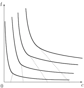
Figure 2 shows an example of agents’preferences in a two-period setting, i.e. for xi 2 R+[ R2+. An agent who lives the …rst period only remains on the horizontal
axis (i.e. second period consumption is zero). The dashed line segments mean that the individual is indi¤erent between the two extreme points of the line segment. The upper end of the dashed segment gives the (constant) consumption that should be given to the agent in each period of a hypothetical two-period life to make him exactly as well-o¤ as he is with a single period of life.
Figure 2 illustrates that, to keep the same satisfaction level while raising the length of life, what is required may possibly be either a smaller or a larger consump-tion per period, depending on the consumpconsump-tion enjoyed while having a short life. For a short-lived individual whose consumption is high (i.e. at the right of the horizontal axis), the consumption that should be given to him in a two-period life to make him indi¤erent with its current state, which is given by the end of the dashed segment, would be much smaller than its current consumption. This re‡ects the attractiveness of a longer life for a person with a high current standard of living. On the contrary, for a short-lived agent whose consumption is low (i.e. at the left of the horizontal axis), the consumption that should be given to him in a two-period life to make him indi¤erent with its current state might be larger than his current consumption. His low current consumption puts him in such a misery that the lengthening of his life
5Note that we do not assume those properties for lives with di¤ erent lengths. For instance,
requiring that the three-periods life (2; 2; 1) be necessarily better than the two-period life (2; 2) would be too strong. One may prefer death to an additional period with consumption equal to 1.
-c
6
d
0
Figure 2: Indi¤erence curves in (c; d) space
with the same consumption per period would make him worse o¤. Hence additional consumption per period is needed to compensate him for having a longer life.
Clearly, all allocations are not equivalent in terms of how short-lived agents are treated. Therefore, in order to provide theoretical foundations to the compensation of short-lived persons, it is necessary to de…ne social preferences over allocations. Such social preferences will serve to compare allocations in terms of their goodness and fairness. Those social preferences will be formalized by a social ordering function
% which associates every admissible preference pro…le RN of the population with an
ordering%RN de…ned on the set of all possible allocations for N , that is, an ordering
de…ned on XjNj. For all xN; yN 2 XjNj, xN %RN yN means that the allocation xN is,
under the preference pro…le RN, at least as good as the allocation yN. The symbols RN and RN will denote strict preference and indi¤erence, respectively.
3
The social objective
This section aims at deriving a social objective that is adequate for the allocation of resources among agents having unequal longevities. As mentioned above, standard social objectives like utilitarianism do not do justice to basic intuitions supporting the compensation of the short-lived, so that we need to look for other objectives. Obviously, there exist many possible social preferences. The only way to select
reasonable social preferences is to impose some plausible ethical requirements that these should satisfy. Such ethical requirements will take here the form of four axioms. The …rst axiom states that if all individuals prefer one allocation to another, then this should also be regarded as socially preferable to that alternative.
Axiom 1 (Weak Pareto) For all preference pro…les RN 2 <jNj, all allocations
xN; yN 2 XjNj, if xiPiyi for all i 2 N, then xN RN yN.
That axiom can be justi…ed on two grounds. First, it seems essential to respect individual preferences in order to address trade-o¤s between, for instance, consump-tion at di¤erent points in life. Second, the Pareto axiom is also a guarantee against the choice of ine¢ cient allocations: it states that any unanimity in the population regarding the ranking of two allocations should be respected by social preferences.
The next axiom requires social preferences to use the relevant kind of information about individual preferences. More precisely, it states that, in order to compare allocations for a given individual, it is su¢ cient to look at the indi¤erence sets of the individual at the consumption pro…les under consideration.
Axiom 2 (Hansson Independence) For all preferences pro…les RN; R0N 2 <jNj
and for all allocations xN; yN 2 XjNj, if for all i 2 N, I(xi; Ri) = I (xi; R0i) and
I(yi; Ri) = I (yi; R0i), then xN %RN yN if and only if xN %R0N yN.
This condition, which was …rst introduced by Hansson (1973) and Pazner (1979), requires that social preferences over two allocations depend only on the individual indi¤erence curves at these allocations. Note, however, that those indi¤erence curves contain more information than individual pairwise preferences over these two alloca-tions. This allows us to avoid Arrow’s impossibility result.
The next two axioms are re…nements of the Pigou-Dalton principle in the context of unequal longevities.
The Pigou-Dalton principle for Equal Preferences and Equal Lifetimes is an im-mediate translation of the Pigou-Dalton principle in the present context. It states that, if we take two allocations such that the consumption pro…les are exactly the same under the two allocations for everyone except for two persons, then, if those two individuals have equal lifetimes and equal preferences, the allocation in which the two agents have, when alive, closer consumption pro…les is more socially desirable than the one in which they have more unequal consumption pro…les.
Axiom 3 (Pigou-Dalton for Equal Preferences and Equal Lifetimes) For all
(xj) = (yj) = `, and if there exists 2 R`++ such that
yi xi = yi xj = yj+ yj
and xk= yk for all k 6= i; j, then
xN %RN yN:
That axiom is pretty intuitive: for agents who are identical in terms of every-thing (i.e. longevities, preferences) except their consumptions, a redistribution from the agent with the higher consumption to the agent with the lower consumption constitutes a social improvement.
While that re…ned version of the Pigou-Dalton principle is intuitive, it is nonethe-less restricted to agents with equal preferences, which is a strong restriction. Actu-ally, we would like also to be able to say whether a consumption transfer is a social improvement or not when agents have di¤erent preferences. Note, however, that making this kind of statement is not trivial, as it is not obvious to see in which case some consumption transfer from a rich to a poor could be regarded as a social improvement whatever individual preferences are.
In the following axiom, it is argued that, if the two agents in question have a longevity that is equal to a level of reference ` , then a transfer that lowers the constant consumption pro…le of the rich and raises the constant consumption pro…le of the poor constitutes a social improvement, whatever individual preferences are. Axiom 4 (Pigou-Dalton for Constant Consumption and Reference Lifetime) For all RN 2 <jNj, all xN, yN 2 XjNj, and all i, j 2 N, such that (xi) = (yi) =
(xj) = (yj) = ` , and xi and xj are constant consumption pro…les, if there exists
2 R`
++ such that
yi xi = yi xj = yj+ yj
and xk= yk for all k 6= i; j, then
xN %RN yN:
The reference longevity level ` can be interpreted in the following way. An ex-ternal observer could, when comparing the lives of two persons with the same length
` , say who is better o¤ than the other by just looking at the constant consumption
pro…les of those agents, without knowing anything about their preferences. Thus, ` is the length of life such that if it is enjoyed by distinct persons, one can compare the well-being of those agents directly from their consumptions (provided they are
constant over time), without caring for their preferences. Note that this axiom is weak. It would be tempting to extend it to cases in which the longevity of the agents can take other values than a particular ` : isn’t it intuitive that a greater constant consumption for any given longevity makes one better o¤? Unfortunately, such an
extension would render the axiom incompatible with Weak Pareto.6 This is why the
axiom can be formulated for at most one reference level of longevity.
There is no need, at this stage, to assign a speci…c level to the reference longevity ` . Intuitively, it makes sense to set ` at the "normal" lifespan, that is, the lifespan that everyone — whatever one’s life-plans are — would like to have, but it is not trivial to see which lifespan is the normal one. Note that the selection of ` may have important redistributive consequences, in combination with the Pareto axiom. Taking, for instance, a maximal lifespan of 120 years as the reference would imply giving priority to those who have a strong preference for longevity. This is because their situation is equivalent, according to their own preferences, to a situation in which they live for 120 years with a low consumption. Given that the "normal" lifespan may vary with the circumstances — in particular with the quality of life (health status) — , we will not …x it, and keep it as an ethical parameter.7
The four ethical principles that are presented above seem quite reasonable. We now have to investigate which kind of social preferences do satisfy these conditions. As we shall see, the answer to that question will be quite precise. But before providing that answer, let us …rst introduce what we shall call the Constant Consumption Pro…le Equivalent on the Reference Lifetime (CCPERL).
De…nition 1 (Constant Consumption Pro…le Equivalent on the Reference Lifetime)
For any i 2 N, any Ri 2 < and any xi 2 X, the Constant Consumption Pro…le
Equivalent on the Reference Lifetime (CCPERL) of xi is the constant consumption
pro…le ^xi such that (^xi) = ` and
xiIix^i:
The CCPERL can be interpreted as a way to homogenize consumptions across individuals having di¤erent longevities, by converting consumptions under di¤erent longevities into some comparable consumptions. The intuition behind that homoge-nization exercise is the following. In the present context, where agents have unequal
6Such an incompatibility between the Pareto principle and the principle of transfer in the
multi-dimensional context is well documented. See, e.g., Fleurbaey and Maniquet (2011). Intuitively, the problem stems from the fact that, at a low common level of longevity, making a progressive transfer from an individual who cares a lot about longevity to another who cares less about longevity may be Pareto equivalent to a regressive transfer at a greater level of longevity — their indi¤erence curves crossing at an intermediate level of longevity.
longevities, looking at individual consumption pro…les does not su¢ ce to have a pre-cise idea of individual well-being. However, the CCPERL does allow to have a more precise view, as it has, by construction, taken longevity di¤erentials into account.
It is trivial to see that, if xi is a constant consumption pro…le with (xi) = ` = ` ,
then ^xi = xi. However, if xi is a constant consumption pro…le (with consumption
level for each life-period equal to ci) with ` < ` , then we have ^xi ? (ci; :::; ci),
depending on whether ci lies above or below the critical level making a longer life
with that consumption worth being lived. The CCPERL of xi always exists if ` = T;
by assumption made on <; but the existence of the CCPERL is not guaranteed if ` < T:It may happen that xi with high longevity is strictly preferred to all lifetime
consumption pro…les with lower longevity ` : When this happens, we adopt the convention that the CCPERL is in…nite. This problem of non-existence is not very important as the social preferences highlighted here focus on the worst-o¤ individuals. Having de…ned the CCPERL, we can now present the following theorem, which characterizes the social preferences, or, more precisely, states that the Maximin on CCPERL is a necessary condition for social optimality.
Theorem 1 Assume that the social ordering function% satis…es Axioms 1-2-3-4 on
<jNj. Then % is such that for all R
N 2 <jNj, all xN, yN 2 XjNj,
min
i2N(^xi) > mini2N(^yi) =) xN RN yN:
In other words, the social ordering satis…es the Maximin property on the Constant Consumption Pro…le Equivalent on the Reference Lifetime (CCPERL).
The proof is in the Appendix. It should be noted that this theorem does not give a full characterization of social preferences because it does not say how to compare allocations for which min (^xi) = min (^yi).8 All the theorem states is that if one
allocation exhibits a higher minimum CCPERL than another, then it must also be socially more desirable. In other words, the theorem implies that maximizing min (^xi)
is a necessary operation, as the best social allocation is necessarily included in the set of allocations that maximize min (^xi).
However, this result tells us a lot about social preferences. True, if the set of allo-cations that maximize min (^xi)is not a singleton, looking at the minimum CCPERL
only would not tell us which allocation is the most desirable. However, in more
8Clearly, given the postulated axioms, the equality of the min (^x
i) for two allocations does not
necessarily imply social indi¤erence between these allocations: an allocation could still be regarded as better than the other (on the grounds of other aspects of the distribution), and the theorem has nothing to say about that.
concrete problems, it is likely that the Maximin on CCPERL has, as a solution, a unique allocation, in which case that allocation must also be the most socially desir-able allocation. When a unique solution is not obtained, it is natural to re…ne the Maximin into the Leximin, which extends the lexicographic priority of the worse-o¤ to higher ranks in the distribution.
While the details of the proof are provided in the Appendix, its overall form can be brie‡y given here. The proof proceeds in two stages. In a …rst stage, it is shown that Weak Pareto, Hansson Independence and Pigou-Dalton for Equal Preferences and Equal Lifetimes imply Hammond Equity for Equal Preferences. That principle states that, if two persons i and j have the same preferences, but i lies on a higher indi¤erence curve than j, pushing i on a lower indi¤erence curve and j on a higher one is socially desirable. This embodies an absolute priority for the worst-o¤. In a second stage, Hammond Equity for Equal Preferences is then used to show that, if we add Pigou-Dalton for Constant Consumption and Reference Lifetime, we obtain Hammond Equity for Reference Lifetime. According to that principle, if two persons
i and j, possibly with di¤erent preferences, have the same longevity equal to the
reference ` , but i has a higher constant consumption pro…le than j, then lowering the constant consumption pro…le of i and raising the one of j is socially desirable.
Let us note that an alternative characterization can be made in a slightly di¤erent setting. Suppose for the rest of this section that longevity is a continuous variable, so that a lifetime consumption pro…le is now described as a function xi(t) de…ned over
the interval [0; T ] : We restrict attention to functions xi(t)which are strictly positive
and continuous over an interval [0; (xi)] and null over the complement ( (xi) ; T ] :
The corresponding longevity is obviously (xi). Individual preferences over lifetime
consumption pro…les xi can still be de…ned and assumed to be convex, continuous
(with respect to the topology of pointwise convergence) and weakly monotonic. The axioms of Weak Pareto and Hansson Independence are immediately adapted to this setting. Let us now introduce a new axiom which states that, whatever the individual preferences, it is always socially desirable to reduce longevity inequalities among agents who enjoy the same consumption per life-period, when one agent lives longer than ` and the other has a shorter life. For this axiom not to be idle, it must be assumed that 0 < ` < T: A similar assumption was not needed with the axiom of Pigou-Dalton for Constant Consumption and Reference Lifetime.
Axiom 5 (Inequality Reduction around Reference Lifetime) For all RN 2
<jNj, all x
N, yN 2 XjNj, and all i, j 2 N, such that (xi) = `i, (yi) = `0i,
of consumption for xi; yi; xj; yj; if
`j; `0j ` `i; `0i and `j `0j = `0i `i > 0
and xk= yk for all k 6= i; j, then
xN %RN yN:
That axiom is quite attractive: reducing longevity inequalities between long-lived and short-long-lived agents who enjoy equal consumptions per period can hardly be regarded as undesirable. Note, however, that the attractiveness of that axiom is not independent from the monotonicity of preferences in longevity. If consumption per period is so low that some agents may prefer having a short rather than a long life, reducing longevity inequalities by raising the longevity of the short-lived may be socially undesirable. Thus this axiom, unlike axioms 3 and 4, must be used in a subdomain of preferences satisfying a stronger monotonicity condition with respect to longevity.
Observe that by weak monotonicity, for every individual preference ordering Ri
and every lifetime consumption pro…le xi; there is a unique constant pro…le with
same longevity such that every pro…le with greater consumption and same longevity is strictly preferred and every pro…le with lower consumption and same longevity is strictly worse. Therefore, by Weak Pareto one can restrict attention to constant lifetime consumption pro…les and work with bundles having two dimensions, namely, per-period consumption and longevity. Formally, Inequality Reduction around Ref-erence Lifetime is then similar to the Free Lunch Aversion Condition proposed by Maniquet and Sprumont (2004) in the context of public goods provision. It is then a simple adaptation of their analysis to show that the conclusion of Theorem 1 holds in this particular setting when it is required that the social ordering function must obey the axioms 1-2-5. The only minor di¤erence is that longevity is here bounded between 0 and T; whereas the corresponding variable (contribution of private good to the production of public good) is unbounded in their model.9
9Although Inequality Reduction around Reference Lifetime is meaningful in the model of this
paper introduced in Section 2, Th. 1 does not hold with axioms 1-2-5, even with stronger monotonic-ity assumptions about individual preferences. The reason is that if the worst-o¤ gains very little, this may not be equivalent to gaining one period of longevity at any level of consumption. Axiom 5 is then powerless because it applies only when the worst-o¤ in the "transfer" of longevity gains at least one period of additional longevity.
4
First-best optimum
The previous section showed that basic axioms on social preferences imply that the optimal allocation must maximize the minimum CCPERL in the population. What are the consequences of this result on the optimum allocation of resources? If, for instance, a social planner could have anticipated, in 1900, the distribution of longevities of Swedish women as shown on Figure 1, how should he have allocated a …xed amount of resources among the cohort members?
This section aims at characterizing the social optimum in a resource allocation problem when the axioms of Theorem 1 are satis…ed. We will also contrast this social optimum with the utilitarian optimum, to see what kinds of compensations the Maximin on CCPERL implies in contrast with the utilitarian allocation.
For such purposes, let us consider a simple model where agents live either one
or two periods.10 The length of life of each agent is only known ex post. Ex ante,
the social planner knows individual preferences and life expectancies, as well as the statistical distribution of longevity in the population, and looks for the optimum allocation of an endowment W of resources.
Individual lifetime welfare takes a standard time-additive form: Uij1 = u(cij);
Uij2 = u(cij) + iu(dij);
EUij = u(cij) + j iu(dij);
where cij and dij denote …rst-period and second-period consumptions of an agent
with a time preference factor i and a survival probability j, while Uij1 and Uij2
denote his actual lifetime utility if he lives respectively one or two periods, and EUij
is the corresponding expected utility. Temporal utility u( ) takes the same form for everyone.11
Heterogeneity here takes the following form. Ex ante, agents di¤er in their at-titude towards the future, i.e. in their time preferences, i, and in their survival probabilities, j, with two types for each parameter:
0 < 1 < 2 < 1; 0 < 1 < 2 < 1:
10The assumption T = 2 is here made for analytical simplicity. We discuss below how robust our
results are to assuming T > 2.
11As usual, we assume: u0(c
Hence, there exist 4 types of agents ex ante, who are di¤erentiated by their i and j. Ex post, there are 8 types of agents, as each ex ante type includes short-lived
and long-lived agents.12
For the sake of presentation, we here adopt three assumptions which will be re-laxed later on (see Section 6). First, we assume that u(0) > 0, so that it is always strictly better to be long-lived rather than short-lived. Note that this assumption is not the standard one (see Becker et al. 2005), but it greatly simpli…es the com-putation of optimal allocations. Second, we assume that the social planner faces a unique intertemporal resource constraint, in the sense that he can allocate resources as …rst-period or second-period consumptions without any cost. Third, we assume that agents cannot transfer resources across periods, so that the bundles (received from the planner) have to be consumed in the same periods as they are received, without any possibility, at the individual level, to reallocate resources over time.
Within that framework, the problem of the social planner consists in o¤ering four consumption bundles (cij; dij) to agents with time preference parameter i and
survival probability j, for i = 1; 2 and j = 1; 2. Note that these bundles do not
depend on whether agents live one or two periods, as the actual length of life is not known ex ante by the planner.
In the following, we …rst solve the problem faced by a utilitarian planner, and then, we contrast it with the Maximin on CCPERL, assuming that the planner can
observe characteristics i and j. We relax this assumption in Section 5.
4.1
Utilitarian optimum
The problem of the utilitarian social planner amounts to selecting bundles (cij; dij)in
such a way as to maximize social welfare ex post, subject to the resource constraint:13
max c11;c12;c21;c22 d11;d12;d21;d22 u (c11) + 1 1u (d11) + u (c21) + 1 2u (d21) +u (c12) + 2 1u (d12) + u (c22) + 2 2u (d22) s.to c11+ 1d11+ c21+ 1d21+ c12+ 2d12+ c22+ 2d22 W
From the …rst-order conditions, we obtain that the optimal allocation is such that c11 = c12= c21= c22 > d21 = d22> d11= d12:
For every agent, the …rst-period consumption exceeds the second-period
consump-tion, since i < 1. Moreover, the …rst-period consumption is equalized across all
12For simplicity, we assume that there is a mass 1 of individuals in each of the ex ante groups. 13In the rest of this paper, we shall refer to classical utilitarianism as merely utilitarianism.
agents. On the contrary, the second-period consumption is di¤erentiated according to their time preferences, but not according to their survival probabilities. Hence, the
second-period consumption is higher for agents with a higher i, but is independent
from j.14
Regarding the ranking of agents in terms of ex post lifetime welfare, it is clear that the worst-o¤ agents are the short-lived, followed by 1-type agents living two periods.
The best-o¤ agents are the 2-type agents living two periods.15 The utilitarian
optimum thus tends to favour long-lived agents over short-lived agents, and patient agents (i.e 2-type) over impatient agents (i.e. 1-type).16
4.2
Maximin on CCPERL
Let us now contrast the utilitarian optimum with the Maximin on CCPERL. For that purpose, we will take the maximum length ` = 2 as a reference level ` . By
de…nition, the CCPERL for an agent of type ( i; j) with an actual length of life
` = 1; 2 is the constant consumption pro…le ^xij` = (^cij`; ^cij`) such that:
u (^cij2) + iu (^cij2) = u (cij) + iu (dij)
u (^cij1) + iu (^cij1) = u (cij)
On the …rst line, ^cij2 de…nes the consumption equivalent of an agent with time
preference i and survival probability j who e¤ectively lived two periods, while the
second line de…nes a consumption equivalent ^cij1 for a ( i; j)-type agent living only
one period. Note that since we take ex-post utilities on the right-hand side of these
expressions, the CCPERL of an agent does not depend on his survival probability.17
Let us …rst de…ne the consumption equivalent ^xij` = (^cij`; ^cij`) for each of the 8
groups of individuals that emerge ex post.
14This result is due to the fact that the survival probability
j enters the social objective and
the budget constraint in the same way.
15Note that since di¤erences in survival do not a¤ect the optimum, this ranking is similar to the
one we would obtain if there was no di¤erence in survival chances.
16This results follows from the additivity of (1) the utilitarian social welfare function and (2)
individual lifetime welfare (see Bommier et al. 2009, 2010). Note, however, that relaxing (2) would not eradicate the utilitarian tendency to favour the long-lived (see Leroux and Ponthiere 2010).
` def. CCPERL ^cij` 1 1 1 u (^c111) (1 + 1) = u (c11) 1 2 1 u (^c121) (1 + 1) = u (c12) 2 1 1 u (^c211) (1 + 2) = u (c21) 2 2 1 u (^c221) (1 + 2) = u (c22) 1 1 2 u (^c112) (1 + 1) = u (c11) + 1u (d11) 1 2 2 u (^c122) (1 + 1) = u (c12) + 1u (d12) 2 1 2 u (^c212) (1 + 2) = u (c21) + 2u (d21) 2 2 2 u (^c222) (1 + 2) = u (c22) + 2u (d22)
Table 1: De…nition fo the consumption equivalents
To …nd the bundles that maximize the minimum CCPERL, we …rst need to identify the worst-o¤ agents. We can …rst note that, as u(0) > 0, short-lived agents are worse-o¤ than long-lived agents of the same type, as death prevented them from enjoying the second period (which is positively valued). From this, it follows that the allocation that satis…es the Maximin on CCPERL is obtained by transferring second-period resources to the …rst period, i.e. by decreasing dij to 0:
d11= d12 = d21 = d22 = 0:
Second, the CCPERL can be equalized among short-lived agents by increasing c2j
and decreasing c1j until one reaches ^c111 = ^c121 = ^c211 = ^c221. This is obtained by
setting c11 = c12 < c21 = c22. Hence, …rst-period consumption is larger for patient agents (i.e. with a high i) as they are more a¤ected by a short life than impatient
agents (i.e. with a low i). Thus, to compensate them, more consumption in the …rst
period is needed. This justi…es the di¤erentiated treatment in terms of consumption between agents with di¤erent time preferences. We obtain the following ranking:
^
c111 = ^c121 = ^c211 = ^c221 < ^c112 = ^c122 < ^c212 = ^c222
under our assumption u (0) > 0. Thus, whereas the Maximin on CCPERL enables us to make some compensation of short-lived individuals, this does not, however, imply a full compensation, because the social planner cannot, ex ante, know the actual lengths of life. Moreover, as the above ranking shows, among the long-lived agents, there is also an inequality due to the larger bene…t of living longer for patient agents.18
18Indeed one has, at the solution of the Maximin on CCPERL that,
u (^c112) =
u (c11) + 1u (0)
1 + 1 < u (^c212) =
u (c21) + 2u (0)
Note that the social planner does not use the information on survival probabilities
j to o¤er distinct consumption bundles to agents with di¤erent life expectancies.
As mentioned earlier, this uniform treatment of agents with di¤erent j comes from
the fact that survival probabilities do not in‡uence the CCPERL, which is de…ned ex post, that is, once the risk of death has been resolved.19 What we do here is to compensate short-lived agents, independently of how unlucky their death was.
All in all, this solution di¤ers strongly from the utilitarian optimum, under which the optimal bundles included a positive consumption in the second period. The following proposition sums up the results of this section.
Proposition 1 Assume that u(0) > 0, and that the social planner faces a unique in-tertemporal budget constraint. Under perfect information about ex-ante types ( i; j):
Utilitarianism equalizes …rst-period consumptions for all agents at a level that exceeds second-period consumptions. Agents with a low impatience bene…t from a higher second-period consumption.
Maximin CCPERL involves higher …rst-period consumptions for patient agents, and lower …rst-period consumptions for impatient agents. Second-period con-sumptions are all set to zero.
Under both criteria, agents who di¤er in their survival probabilities but have the same preferences are treated identically. The introduction of heterogeneity in survival probabilities does not alter the optimal allocation.
5
Second-best optimum
Up to now, we assumed that individual characteristics i and j were perfectly
ob-servable by the social planner. This section reexamines the utilitarian and egalitarian-equivalent solutions under asymmetric information, that is, when agents know their
( i; j)-type, while the government only observes the distributions of types. The
government can still propose di¤erent bundles to ex ante groups, but under the constraint of incentive compatibility.
with c11< c21 and 1< 2. The same reasoning applies for u (^c122) < u (^c222).
5.1
Utilitarian optimum
As we saw above, the utilitarian planner does not want, under perfect information, to give priority to agents on the basis of their survival probability: agents di¤ering only
in j were all treated equally in the …rst-best utilitarian optimum. However, under
asymmetric information, one cannot exclude a priori a di¤erentiation of bundles on the basis of j. Indeed, survival probabilities j now a¤ect also the planner’s problem
by their presence in the incentive compatibility constraints.
To study the utilitarian problem under asymmetric information, we shall, for simplicity, focus here on the case where the di¤erence in patience looms larger than the di¤erence in survival probabilities:
1 1 < 2 1 < 1 2 < 2 2
The agents’preferences satisfy the single-crossing property in the corresponding
or-der. If the social planner proposed the …rst-best allocation, 1-type agents would
like to mimic 2-type agents, independently of their survival chances. Hence, using
also the above inequalities, the relevant incentive compatibility conditions are:20 u (c11) + 1 1u (d11) u (c12) + 1 1u (d12) ;
u (c12) + 2 1u (d12) u (c21) + 2 1u (d21) ;
u (c21) + 1 2u (d21) u (c22) + 1 2u (d22) :
Under the single-crossing property, these three incentive compatibility constraints su¢ ce to avoid any mimicking behaviour. Intuitively, it must be the case that the optimal second-best allocation is such that agents with type ( 1; 1)receive the
highest …rst-period consumption and the lowest second-period consumption, followed by the other types as follows:
c11 c12 c21 c22;
d11 d12 d21 d22:
20If agents had the same survival chances, there would be only one incentive constraint,
u (c1) + 1u (d1) u (c2) + 1u (d2) ;
This ensures that impatient agents would not mimic patient ones under asymmetric information. As usual in this type of problem, the allocation of the mimicker (with time preference 1) would not be distorted. But the second-period consumption of 2-type agents would increase and their …rst-period consumption would decrease with respect to the …rst-best, in such a way as to relax an (otherwise binding) self-selection constraint. Hence, we would have: d1< c1, c2< c1 and c27 d2:
Let us now check whether the planner, in contrast with the …rst-best optimum, wants to di¤erentiate between agents on the basis of their survival probabilities. The problem of the planner is equivalent to the …rst-best problem, to which we add the
above incentive constraints. Rearranging the FOCs of the ( 1; 1)-type agents, we
obtain the usual result of no distortion at the top for the extreme mimicker: u0(c11) = 1u0(d11):
This trade-o¤, which is similar to the one we had in the …rst-best, yields c11 > d11.
On the contrary, for other agents (and eliminating from these equations the Lagrange multiplier associated with the resource constraint), we now have:
u0(c 12) 1u0(d12) = 1 1 1 2 + 2 1 1+ 2 u0(c 21) 2u0(d21) = 1 2 2 1 1 2 + 3 1 2+ 3 u0(c 22) 2u0(d22) = 1 3 1 2 1 3 :
where k; k = 1; 2; 3 are the Lagrange multipliers associated with the incentive
compatibility constraints. The possibility of mimicking behaviors then leads the planner to give distinct bundles to agents who have not only di¤erent time preferences but also di¤erent survival chances. For instance, bundles (c11; d11)and (c12; d12) are
di¤erent whenever the (corresponding) …rst incentive constraint is binding (i.e. 1 > 0). However, from these equations it is impossible to exclude the possibility of bunching among the other agents.
Let us now see how these incentive constraints modify the optimal allocation of each type. As the right-hand sides of these expressions are all greater than one, incentive constraints push toward more consumption in the second period for all types, in such a way as to discourage these agents from pretending to be "apparently patient" (apparent patience may be due to a high i or a high j). To see this, let us
study the …rst equation. The trade-o¤ between (c12; d12)is distorted upward so as to
avoid mimicking from ( 1; 1)-type agents. Indeed, it is optimal to encourage
second-period consumption for ( 1; 2)-type agents as compared to the …rst-best trade-o¤,
in order to discourage ( 1; 1)-type agents from pretending to be of that type. By
doing so, this bundle becomes less interesting to ( 1; 1)-type agents, as they would
obtain too much consumption in the second period and not enough in the …rst one, given that they face a lower survival chance 1 < 2. Hence, if 1 = 2, ( 1; 1
)-type agents and ( 1; 2)-type agents would be identical, and we would obtain the
…rst-best trade-o¤.21
In comparison with the …rst-best, the relative di¤erence between …rst-period and second-period consumptions is lower, as the introduction of incentive constraints pushes towards more consumption in the second period. Yet, very little can be said on welfare inequalities between agents with di¤erent types. As compared to the …rst-best, short-lived agents are no longer treated equally, as …rst-period consumptions may now be di¤erent for individuals with di¤erent ( i; j).
Moreover, under asymmetric information, short-lived agents are still worse-o¤ than the long-lived, and this inequality may even be increased by the introduction of incentive constraints, as it encourages consumption in the second period. Also, among long-lived agents, it is not sure who would end up with the highest welfare.
5.2
Maximin on CCPERL
As in the …rst-best, we take the maximum length ` = 2 as the reference level ` for de…ning the CCPERL. Let us …rst recall that in the …rst-best, …rst-period con-sumptions are distributed among agents only according to their time preferences, and second-period consumptions are set to zero. Hence, under asymmetric
informa-tion, independently of their survival chance j, only type- 1 agents would like to
mimic type- 2 agents, so that the second-best allocation now has to also satisfy the
following incentive compatibility constraint,
u (c1j) + j 1u (d1j) u (c2j) + j 1u (d2j), 8j
The …rst-best egalitarian-equivalent optimum, with c11 = c12 < c21 = c22 and
dij = 0for all i; j; is not incentive-compatible because it violates the above condition.
As the Maximin on CCPERL focuses on short-lived agents, it still makes sense to keep dij = 0, but we now need, in order to satisfy the incentive constraint, to equalize
…rst-period consumptions. In sum, the second-best Maximin CCPERL solution is: c11 = c12= c21 = c22> d11 = d12 = d21= d22= 0: As a consequence, we have ^ c211 = ^c221 < ^c111 = ^c121 < ^c112 = ^c122; ^ c211 = ^c221 < ^c212 = ^c222: 21The same reasoning applies for the other trade-o¤s.
In comparison with the …rst-best, it is no longer possible to equalize the consumption-equivalent of short-lived agents, as this would require consumption inequalities that violate the incentive-compatibility constraint. Moreover, it is no longer always true that ^c212 and ^c222 are the greatest, because now cij = c for all i; j; and 1 < 2.
Let us brie‡y sum up the results of this section.
Proposition 2 Assume that u(0) > 0, and that the social planner faces a unique
intertemporal budget constraint. Under asymmetric information about ex ante types ( i; j):
Utilitarianism gives a …rst-period consumption greater than the second period consumption to agents with a low patience or low survival probability. For the other agents, the introduction of incentive constraints pushes towards more consumption in the second period. Individual bundles should be di¤erentiated according to their time preference but also according to their survival chance. We may have pooling for some types.
Maximin CCPERL involves a perfect equalization of …rst-period consumptions for all agents. Second-period consumptions are all equal to zero.
A common feature of the utilitarian and egalitarian-equivalent solutions is that consumptions are, under each social objective, not smoothed across time. Never-theless, second-period consumptions are zero in the egalitarian-equivalent solution, whereas they are strictly positive under utilitarianism, so that the departure from a smoothed consumption is much larger under the egalitarian-equivalent solution. Hence welfare inequalities between short-lived and long-lived agents are larger under utilitarianism than under the egalitarian-equivalent solution. Moreover, under utili-tarianism, …rst-period consumptions are not equalized across agents, whereas under the egalitarian-equivalent solution, …rst-period consumptions are equalized. This dif-ference comes from the fact that, under utilitarianism, the distortion induced by the incentive constraints acts on both …rst-period and second-period consumptions. On the contrary, under the egalitarian-equivalent solution, the distortion must be only on the …rst-period consumption, as changing second-period consumptions would raise inequalities between short-lived and long-lived agents.
6
Extensions and generalisations
As shown in the previous sections, the Maximin on CCPERL yields rather extreme solutions. The optimal allocation is a corner solution, as it involves zero
second-period consumption. In this section, we propose to check whether the speci…c as-sumptions we made in Sections 4 and 5 are responsible for this result. For this purpose, in this section we will relax di¤erent assumptions successively, and discuss the robustness of the solution to those changes.
Firstly, we will consider more general preferences, by relaxing the assumption of a positive utility of survival (i.e. u(0) > 0). Secondly, we discuss the possibility of adopting a reference lifetime ` lower than maximum longevity (i.e. 2 periods). Finally, while we assumed so far that the social planner controlled the allocation of resources over time, we will consider the case where agents can freely transfer resources across periods.
6.1
The utility of survival
Let us …rst assume that the utility of zero consumption is zero: u (0) = 0. In this case, the individual does not gain any utility from his mere survival. Obviously, Table 1 is independent of the assumption on u (0), so that our previous reasoning still holds. Thus, in the …rst-best egalitarian-equivalent optimum, we obtain that
c11 = c12 < c21 = c22
d11 = d12 = d21 = d22 = 0
The only di¤erence with respect to the case where u(0) > 0 comes from the rank-ing of agents in terms of CCPERL. We now have that all CCPERL are equalized across agents with di¤erent lengths of life, di¤erent survival probabilities and di¤er-ent time preferences, unlike the case with u(0) > 0 (for which long-lived agdi¤er-ents had higher consumption-equivalents). The assumption u(0) = 0 allows for a complete compensation of short-lived agents.
Let us now turn to the second-best (asymmetric information). As the …rst-best allocation under u(0) = 0 is identical to the one under u(0) > 0, incentive constraints are also identical, so that it still optimal to provide cij = c and dij = 0. Again, only
the ranking in terms of CCPERL changes: ^
c111 = ^c121 = ^c112 = ^c122 > ^c211 = ^c221 = ^c212 = ^c222
which, looking at Table 1, is a direct consequence of the di¤erences in time prefer-ences. Our results are summarized in the following proposition.
Proposition 3 Assume that u(0) = 0. In the …rst-best, the CCPERL is equalized
…rst-period consumption to patient agents. In the second-best, the optimal allocation consists in giving the same …rst-period consumption to all agents and zero second-period consumption.
Let us now turn to the case in which u (0) < 0, and de…ne d as the level of consumption such that u (d ) = 0. The …rst-best optimum still equalizes CCPERL across all agents, but is now modi…ed. Three cases should be distinguished, depend-ing on how large the available resources W are.
If W > d [4 + 2 ( 1+ 2)], it is optimal to …x second-period consumptions to
d , and to give a higher …rst-period consumption to patient agents. That allocation
equalizes CCPERL across agents with unequal longevities, because living a second period with d or not is a matter of indi¤erence. Note that, while the positive second-period consumption induced by u(0) < 0 may seem to make the egalitarian-equivalent solution less "extreme" than before, it remains that this solution only assigns long-lived agents a consumption that makes their survival equivalent to death. Thus, even if the Maximin CCPERL seems less extreme than in the benchmark case, the underlying idea is the same: fully compensating short-lived agents implies making the survival of long-lived agents worthless. If, alternatively, d 2 ( 1+ 2) < W <
d [4 + 2 ( 1+ 2)], the Maximin CCPERL gives d as second-period consumption,
and a …rst-period consumption lower than d , with a higher level for patient agents. Finally, if W < d 2 ( 1+ 2)), it is optimal to have a second-period consumption as
close as possible to d , while …xing …rst-period consumption to 0.
Consider now the asymmetric information context, and focus on the case in which
W > d [4 + 2 ( 1+ 2)]. The second-best optimum does not necessarily consist in
giving d to all old agents and an identical bundle c to all young agents. Suppose, for instance that 1 is close to zero. By o¤ering a menu of two bundles, (c ; d ) and
(c + "; 0), for a (not too) small ", one may induce the impatient agents to choose the latter. This frees resources and makes it possible to achieve a larger c than if the same bundle (c ; d ) was o¤ered to everyone. The worst-o¤ agents are the patient agents who choose (c ; d ), whether they die young or survive, and it is then worth maximizing c in order to maximize the lowest CCPERL. Note that in this con…guration compensation for a short life is over-achieved among impatient agents: those who die early are better o¤. Our results are summarized below.
Proposition 4 Assume that u(0) < 0 and that W > d [4 + 2 ( 1+ 2)]. In the
…rst-best, the CCPERL is equalized across all agents by …xing the second-period con-sumption to d , and by giving a higher …rst-period concon-sumption to patient agents. In the second-best, the optimal allocation does not necessarily consist in giving the same consumption to all young agents and d to all old agents.
Finally, it should be stressed that the intercept of the temporal utility function plays a more important role when we consider a general framework with T > 2 life-periods. Indeed, in that case, a strictly positive intercept u(0) > 0 would, under time-additive lifetime welfare, lead to large di¤erentials between the welfares of short-lived and long-lived agents, since the utility from mere survival would accumulate over time for survivors. Hence, under u(0) > 0, the Maximin CCPERL would only provide
partial compensation. However, if we make the more plausible assumption u(0) 0,
then the extension to T > 2 periods would not prevent a complete compensation to short-lived agents. In that case, the consumption at all ages beyond the …rst deaths would be equal to subsistence consumption d , yielding, by de…nition, no welfare gain from surviving one or many extra life-periods.
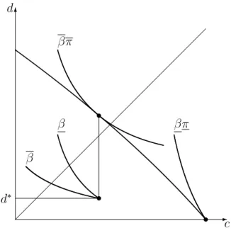
A graphical analysis is helpful. We shall focus here on the second-best optimum.
Let us now assume a distribution of 2 ; and of 2 [ ; ].22 Incentive
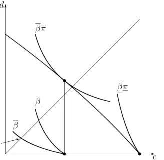
constraints impose to give all agents (who cannot be distinguished ex ante by the planner) the same budget set, represented by the decreasing line in Figure 4 below. The optimistic ( ) patient ( ) agents choose the bundle (c; d), that is, from all chosen bundles, the farthest on the left, while the pessimistic impatient ( ; ) agents choose the bundle that is the most on the right.
Let us …rst focus on the case in which u(0) = 0, which is illustrated in Figure 4. The CCPERL index, with ` = 2, is computed as the solution to
u(^c) + u(^c) = u(c) + u(d) if the agent lives two periods,
u(^c) + u(^c) = u(c) if the agent lives one period.
We then compare the welfare of the agents who consume (c; d) and those who consume c and die. It is clear from above that, for given preferences, the latter are the worst-o¤ since u(d) > 0 when d > 0. For the short-lived agents, the intersection between the indi¤erence curve containing the point (c; 0) and the 45 line gives the
level of ^c. Graphically, the worst-o¤s, ex post, are those who belong to the ;
group and die young, as they have the smallest ^c (i.e. the closest to the left). The
arrow on the …gure shows the CCPERL index for those individuals.23
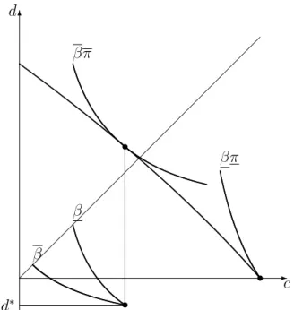
Let us now consider the case in which u(0) > 0. Again, for given preferences, the worst-o¤ agents are those who die young (because u(d) > 0). In order to visualize their situation, it is convenient to extend u ( ) to negative values, and to …nd d < 0
22This does not change the analysis as long as we assume that there are agents with characteristics
; .
23In Figure 4, from point (c; 0), we draw the indi¤erence curves of short-lived individuals with
same survival prospects but with di¤erent , to make explicit that individuals with are worse-o¤ than if they had (i.e., indi¤erence curves are steeper in the latter case).
-6 c d s s s :
Figure 3: Illustration of the argument when u(0) = 0.
such that u(d ) = 0: For short-lived agent one then computes the CCPERL by solving:
u(^c) + u(^c) = u(c) = u(c) + u(d ):
Looking at Figure 5, this corresponds to …nding the point (c; d ) and drawing the indi¤erence curve that goes through that point. The intersection with the 45 line
gives the agent’s CCPERL. Again, ex post, the worst-o¤ are the ; type who die
young, as again their CCPERL are the closest to the left.
From this graphical analysis, it is easy to recover the analytical results of the previous section about the second-best policy. Moreover, one can also obtain a simple way to evaluate arbitrary policies, by observing that the CCPERL of the short-lived
; -type depends only on the …rst-period consumption of this type, which is the
lowest by incentive compatibility.
Proposition 5 If u(0) 0; the comparison of two budget sets is made as follows:
the better budget set is the one that induces the larger level of lowest …rst-period consumption.
-6 c d s s s d
Figure 4: Illustration of the argument when u(0) > 0.
Let us …nally illustrate the case in which u(0) < 0. We now de…ne d > 0 such that u(d ) = 0. We …rst consider the "normal" case in which all agents choose a point (c; d) such that c d and thus u (c) > 0. If d > d , then, for given preferences, the worst-o¤s are still those who die young, because u(d) > 0. Figure 6 illustrates that case. If, on the contrary, one had d < d , the worst-o¤ agents would be the long-lived agents.
When some agents choose (c; d) such that c < d , the worst-o¤ are not
neces-sarily agents with characteristics ; ;depending of the precise con…guration, but
certainly the worst-o¤ agents are among those who choose in this way. Indeed, their CCPERL index is then less than d (whatever the reference longevity), whereas those
who choose (c; d) such that c d have a CCPERL index at least as great as d :
6.2
Reference longevity
Let us now examine the sensitivity of the Maximin CCPERL solution to the longevity level chosen as a reference. As shown in Section 3, the CCPERL is constructed for a particular reference longevity level, at which comparisons in terms of dominance
-6 c d s s s d
Figure 5: Illustration of the argument when u(0) < 0.
of consumption bundles can be made independently of the agents’preferences over longevity. Given that there are several candidates for the reference longevity level, it makes sense to study the robustness of our solution to this reference.
Until now, we have assumed that the reference longevity was the maximum length of life, i.e. ` = 2, and computed the CCPERL for all individuals on the basis of that reference longevity. Let us now assume, alternatively, that the reference longevity ` is the minimum longevity (i.e. 1 period). Under this assumption, Table 1 becomes:
` def. CCPERL ^cij` 1 1 1 u (^c111) = u (c11) 1 2 1 u (^c121) = u (c12) 2 1 1 u (^c211) = u (c21) 2 2 1 u (^c221) = u (c22) 1 1 2 u (^c112) = u (c11) + 1u (d11) 1 2 2 u (^c122) = u (c12) + 1u (d12) 2 1 2 u (^c212) = u (c21) + 2u (d21) 2 2 2 u (^c222) = u (c22) + 2u (d22)
Table 2: CCPERL for reference longevity l*=1
For simplicity, we will assume here that u (0) > 0. In order to …nd the bundles maximizing the minimum CCPERL, we …rst need to identify the worst-o¤ individ-uals. Here again it is clear that the long-lived individuals are better-o¤ than the short-lived individuals. Therefore the optimal allocation must have
d11 = d12= d21= d22= 0
It is also obvious that equalizing the CCPERL of the short-lived individuals is achieved by equalizing their consumption. One must therefore have
c11= c12= c21 = c22= c
Note that this equalization of all …rst-period consumptions di¤ers from what prevailed under ` = 2, where patient agents received a higher …rst-period consump-tion than impatient agents. The reason is that, when the reference longevity is the minimum longevity (i.e. under ` = 1), the CCPERL of the short-lived becomes in-dependent from time preferences, contrary to what was the case when the reference longevity was assumed to be the maximum longevity. Actually, when the reference longevity is one period, all short-lived agents become equal, whether they are patient or not, and this explains why they all have the same compensation.
Note that our …rst-best optimum is also incentive compatible, and, therefore, optimal in the second-best context.
Proposition 6 Assume that u(0) > 0, and that the social planner faces a unique
intertemporal budget constraint. In the …rst-best, the Maximin CCPERL under ` = 1 equalizes all …rst-period consumptions, and sets all second-period consumptions to zero. In the second-best, the Maximin CCPERL under ` = 1 coincides with the …rst-best allocation and is exactly the same as under ` = 2.
In sum, this subsection reveals that the choice of a particular reference longevity level has some e¤ects on the …rst-best egalitarian-equivalent solution, but is less cru-cial in the second-best context. All in all, one should not exaggerate the in‡uence of the reference longevity on the Maximin CCPERL solution. Whatever ` , it keeps the property of decreasing optimal consumption pro…les, in such a way as to compensate short-lived agents.24
6.3
Savings
Up to now, we have assumed that agents could not save resources from one period to the other, or, equivalently, that their savings were controlled by the social planner. In this section, we relax that assumption and assume that savings are completely free. For simplicity, we keep the assumption u (0) > 0.
Now the planner must, at the beginning of the …rst period, give an endowment to individuals, which they can freely allocate between their two periods of life. We
denote by Wij the amount of resources the social planner gives to individuals with
time preference factor i and survival probability j.25
Hence, when the social planner provides Wij to agents, they …rst decide how
to allocate it between …rst-period and second-period consumptions, by solving the problem:
max u (cij) + i ju (dij)
s. to cij + dij Wij;
so that the indirect utility function of a ( i; j)-type agent is
Vij(Wij) = u (cij(Wij)) + i ju (dij(Wij)) ;
where cij(Wij) ; dij(Wij) are obtained from solving the agent’s problem. It is clear
from this maximization problem that, if Wij = W for all i; j, we would have
d11 < d12; d21 < d22, as impatient agents with a lower survival probability prefer
to consume more in the beginning of their life. In this alternative setting, we rede-…ne the consumption equivalent ^cij` for each of the 8 groups of agents:
24Similarly, one could explore variants to the reference to a constant consumption in the de…nition
of CCPERL, without …nding much change to the main policy conclusions.
25Note that, since these resources are allocated at the beginning of the …rst period, the social
planner cannot distinguish between agents who live long and those who die in the end of the …rst period. This will has consequences on the optimal allocation, as we shall see.
` def. CCPERL ^cij` 1 1 1 u (^c111) (1 + 1) = u (c11(W11)) 1 2 1 u (^c121) (1 + 1) = u (c12(W12)) 2 1 1 u (^c211) (1 + 2) = u (c21(W21)) 2 2 1 u (^c221) (1 + 2) = u (c22(W22)) 1 1 2 u (^c112) (1 + 1) = u (c11(W11)) + 1u (d11(W11)) 1 2 2 u (^c122) (1 + 1) = u (c12(W12)) + 1u (d12(W12)) 2 1 2 u (^c212) (1 + 2) = u (c21(W21)) + 2u (d21(W21)) 2 2 2 u (^c222) (1 + 2) = u (c22(W22)) + 2u (d22(W22))
Table 3: Consumption equivalents when individuals can save.
Long-lived agents are better-o¤ than short-lived ones given u(0) > 0. The planner can equalize the CCPERL of the short-lived agents by distributing W11; W12; W21; W22
such that for some ; for all i; j;
u (cij(Wij))
1 + i = :
As c11(W ) > c12(W ) and c21(W ) > c22(W ); this implies that
W11 < W12 and W21 < W22:
If 1 2 < 2 1 (i.e. di¤erences in patience are more important than di¤erences in
survival probabilities), one has c12(W ) > c21(W ): In order to obtain
u (c12(W12))
u (c21(W21))
= 1 + 1
1 + 2;
which implies c12(W12) < c21(W21), one must have W12< W21: In sum, we have
W11< W12 < W21< W22:
There are two main di¤erences with respect to the standard case (Section 4.2). First, the planner now di¤erentiates bundles also with respect to survival probabil-ities, contrary to the case where agents could not save. The planner now takes into account that, when agents can transfer resources to the second period, their actual consumption in the …rst period depends both on their time preferences and on their survival chances. Hence, agents who die early are more penalized by death when they had better survival prospects because they saved more. Second, inequalities in CCPERL between short-lived and long-lived agents are larger than in the standard
case. This is due to the fact that, since Wij is given to agents before they know
their length of life, agents always save some resources for the second period (thus
dij > 0 for survivors). The compensation made by the planner is then limited by
the possibility of individual savings. For the same reason, it is no longer possible to equalize the CCPERLs of long-lived agents with equal preferences.
Finally, we solve the problem under asymmetric information. If the planner were to propose the …rst-best bundles, individuals would always have interest in claiming
to be a ( 2; 2)-type agent. Hence, in order to solve the incentive problem, the
optimum requires that the allocation is such that W11= W12 = W21= W22:
All possibilities of compensatory redistribution are gone in this context. This gener-ates the following ranking among short-lived agents (assuming 1 2 < 2 1):
^
c111 > ^c121 > ^c211 > ^c221:
Proposition 7 summarizes our results (compare with Proposition 2):
Proposition 7 Assume that u(0) > 0, and that both the social planner and agents
face a unique intertemporal budget constraint. In the …rst-best, the Maximin CCPERL
di¤erentiates individual endowments Wij according to time preferences and survival
probabilities. In the second-best, the Maximin CCPERL gives the same bundle to all. Assuming that agents can save at the same rate as the government nulli…es the possibilities of compensation between long-lived and short-lived agents. This should be viewed as an extreme case, as the opposite extreme from the assumption that the agents cannot save at all. In the intermediate case in which the planner can tax savings and redistribute the proceeds, without being able (for technical or political reasons) to impose a prohibitive tax, the optimal policy under CCPERL would adopt the greatest admissible tax in order to maximize …rst-period consumptions.
7
Concluding remarks
Can one compensate the dead? Such a compensation seems impossible: short-lived persons are hard to identify ex ante, and, once dead, it is too late. However, this study provides a positive answer: one solution is to allocate resources ex ante in such a way as to maximize the minimum Constant Consumption Pro…le Equivalent on the Reference Lifetime. The Maximin CCPERL solution involves, in general, declining